HAL Id: hal-02530338
https://hal.archives-ouvertes.fr/hal-02530338
Submitted on 2 Apr 2020
HAL is a multi-disciplinary open access
archive for the deposit and dissemination of sci-entific research documents, whether they are pub-lished or not. The documents may come from teaching and research institutions in France or abroad, or from public or private research centers.
L’archive ouverte pluridisciplinaire HAL, est destinée au dépôt et à la diffusion de documents scientifiques de niveau recherche, publiés ou non, émanant des établissements d’enseignement et de recherche français ou étrangers, des laboratoires publics ou privés.
Robustified expected maximum production frontiers
Abdelaati Daouia, Jean-Pierre Florens, Léopold Simar
To cite this version:
Abdelaati Daouia, Jean-Pierre Florens, Léopold Simar. Robustified expected maximum production frontiers. Econometric Theory, Cambridge University Press (CUP), In press, �10.1017/S0266466620000171�. �hal-02530338�
Robustified expected maximum production frontiers
Abdelaati Daouiaa, Jean-Pierre Florensa and L´eopold Simarb a Toulouse School of Economics, University of Toulouse Capitole, France
b Institut de Statistique, Biostatistique et Sciences Actuarielles, Universit´e Catholique de Louvain, Belgium.
Abstract
The aim of this paper is to construct a robust nonparametric estimator for the produc-tion frontier. We study this problem under a regression model with one-sided errors where the regression function defines the achievable maximum output, for a given level of inputs-usage, and the regression error defines the inefficiency term. The main tool is a concept of partial regression boundary defined as a special probability-weighted mo-ment. This concept motivates a robustified unconditional alternative to the pioneering class of nonparametric conditional expected maximum production functions. We prove that both the resulting benchmark partial frontier and its estimator share the desirable monotonicity of the true full frontier. We derive the asymptotic properties of the par-tial and full frontier estimators, and unravel their behavior from a robustness theory point of view. We provide numerical illustrations and Monte Carlo evidence that the presented concept of unconditional expected maximum production functions is more efficient and reliable in filtering out noise than the original conditional version. The methodology is very easy and fast to implement. Its usefulness is discussed through two concrete datasets from the sector of Delivery Services, where outliers are likely to affect the traditional conditional approach.
Key words : Boundary regression, Expected maximum, Nonparametric estimation, Production function,
Robustness.
1
Introduction
The conventional microeconomic theory of the firm is based on the assumption of optimizing behavior. It is assumed that producers optimize their production choices by avoiding wasting
resources. Theoretically, producers shall operate somewhere on the upper boundary, rather than on the interior, of their production possibility set
Ψ “ tpx, yq P Rp`ˆ R`| y can be produced by xu .
The upper boundary of Ψ, referred to as production frontier or surface, represents the set of the most efficient firms. The economic performance of a firm is defined in terms of its ability to operate close to or on the production frontier. This efficient frontier is often described by the graph of the function ϕpxq “ supty | px, yq P Ψu, which gives the maximal level of output (e.g., a quantity of goods produced) attainable by a firm operating with a vector of inputs x (e.g., labor, energy, capital). The efficiency of a unit working at px, yq may then be estimated via the distance between its production level y and the optimal level ϕpxq. The standard Farrell-Debreu efficiency score is given by the ratio y{ϕpxq, so that an efficiency equal to one corresponds to an output-efficient unit. More generally, the score y{ϕpxq ď 1 gives the increase of output that the firm should reach to be viewed as output-efficient.
The estimation of the frontier function ϕ from a random sample of production units tpX1, Y1q, . . . , pXn, Ynqu is thus of utmost importance in production econometrics. A large amount of literature is devoted to this problem, where two different approaches have been mainly developed: the deterministic frontier approach which supposes that all the obser-vations pXi, Yiq belong to Ψ with probability 1, and the stochastic frontier approach where random noise allows some observations to be outside Ψ. The issue of stochastic frontier estimation goes back to the works of Aigner et al. (1977) and Meeusen and van den Broeck (1977). Typically, it is assumed that ϕ has a parametric structure like Cobb-Douglas or translog. The estimation techniques include modified least-squares and maximum likelihood methods, see for instance Greene (2008) for a survey. Some attempts have been proposed to relax the parametric restriction such as, for instance, Kumbhakar et al. (2007) and Simar and Zelenyuk (2011), see also Kneip et al. (2015) and the references therein.
Our contribution in this paper is related to the context of inference for deterministic production frontiers, where it is assumed that ϕ is nondecreasing. A pioneering contribution in this area is due to Farrell (1957), who introduced Data Envelopment Analysis (DEA), based on either the conical hull or the convex hull of the data. This was further extended by Deprins et al. (1984) to the Free Disposal Hull (FDH) estimator, whose properties have been extensively discussed in the literature. See for instance Kneip et al. (2008) and Daouia et al. (2010, 2014) for a recent survey of the available results. The most appealing charac-teristic of such frontier estimators is that they rely on very few assumptions, but they are by construction very sensitive to outliers. To remedy this vexing defect, robust extensions using a concept of partial production frontiers have been suggested. Instead of estimating the true
full frontier ϕ itself, the idea is to first estimate a partial frontier of the production set Ψ and then shift the obtained estimator to the right place. Prominent among these develop-ments are the concepts of conditional expected maximum production frontiers by Cazals et al. (2002) and conditional quantile-based frontiers by Aragon et al. (2005) and Daouia and Simar (2007). Comparisons between the two concepts from a robustness and an asymptotic point of view can be found in Daouia and Ruiz-Gazen (2006) and Daouia and Gijbels (2011). In particular, once the conditional quantile-based frontiers break down for large chosen tail probability levels, they become definitely less resistant to outliers than the conditional ex-pected maximum output frontiers. Moreover, the latter class of partial production functions has the additional advantage to make more efficient use of the available data since its relies on the distance to observations, whereas quantiles only use the information on whether an observation is below or above the predictor.
Yet, the class of conditional expected maximum output frontiers is not without disadvan-tages. First, it is not constrained to inherit the requisite theoretical axiom of monotonicity of the true full production function ϕpxq. Economic considerations lead actually to the gen-eral production axiom of free disposability of inputs and outputs, that is, if px, yq P Ψ then px1, y1q P Ψ for any x1 ě x and y1 ď y. The monotonicity of ϕpxq, referred to as non-negative marginal productivity, is justified by the free disposability assumption and is a minimal re-quirement in production theory [see, e.g., Gijbels et al. (1999) and Park et al. (2000)]. The conditional expected maximum production function enjoys the property of monotonicity if and only if the non-standard conditional distribution function of Y given X ď x is nonin-creasing in x [see Theorem A.3 in Cazals et al. (2002)]; this necessary and sufficient condition is referred to as tail monotonicity [see, e.g., Gijbels and Sznajder (2013)]. Second and most importantly, even if the theoretical hypothesis of tail monotonicity is satisfied, the empirical estimators of the conditional expected maximum production function, needed to be used in practice, are not constrained to enjoy the property of monotonicity. Third, a desirable prop-erty of any benchmark partial frontier is to closely parallel the true production frontier, as argued by Wheelock and Wilson (2008) and Daouia et al. (2017). However, by construction, both population and empirical conditional, expected maximum output frontiers diverge from the true full frontier as the input level increases [see, e.g., Daouia and Gijbels (2011)]. In particular, similarly to the FDH boundary, the estimated partial frontiers tend to envelop production units with ‘small’ inputs-usage including outliers, and are thus very non-robust to such observations. However, in contrast to the FDH frontier, they may lie below some relatively inefficient production units with ‘large’ inputs-usage. This opposite behavior for ‘small’ and ‘large’ inputs makes the selection in practice of an appropriate benchmark par-tial frontier a hard problem. Also, measuring the distance of production units relative to a
conditional expected maximum production frontier may result in misleading efficiency scores accordingly. All of these limitations come from the reliance of expected maximum produc-tion funcproduc-tions on the condiproduc-tioning by the event tX ď xu, which involves a division by an estimate of PpX ď xq.
In this paper we adopt a different strategy based on a robustified unconditional formu-lation of expected maximum production functions. This new formuformu-lation has an analogous interpretation to the original conditional concept and corrects all of its vexing defects. The proposed unconditional expected maximum output frontiers and their estimators share the desirable property of monotonicity without resorting to the hypothesis of tail monotonicity or any other assumption. Another substantial advantage of these new partial production boundaries over the traditional conditional approach is that they do not suffer from border and divergence effects for small or large levels of inputs. Thanks to this benefit and because monotonicity eliminates sharp changes in the slope and curvature of the built unconditional partial frontiers, the selection problem of an appropriate benchmark frontier tends to be easier than conditional unconstrained partial boundaries. We derive the asymptotic distri-butional behavior of the resulting frontier estimators (both full and partial) by using simpler arguments relative to the standard conditional method. The superiority of our method is also established from a robustness theory point of view. To illustrate the discussed ideas, we use two concrete datasets from the sector of Delivery Services and a third dataset from the Ecuadorian manufacturing sector, where outliers are likely to affect the traditional con-ditional method. The first dataset involves 4,000 French post offices observed in 1994. It has been discussed in Cazals et al. (2002), Aragon et al. (2005), and Daouia et al. (2010, 2012) among others. The second dataset comprises 2,326 European post offices observed in 2013. For each post office i, the input Xi represents the labor cost measured by the quantity of labor, and the output Yi is the volume of delivered mail in number of objects. The third dataset from Daouia and Park (2013) consists of 406 firms in the petroleum, chemical and plastics industries in Ecuador in 2002. The scatterplots are given below in Figures 1, 2 and 7. The paper is further organized as follows. In Section 2, we present a deeper discussion on the concept of expected maximum production functions. We provide the main results includ-ing robustness and asymptotic properties. In Section 3, we explore the estimation method through our motivating real data examples. Section 4 gives some numerical illustrations and Monte Carlo evidence. Section 5 concludes.
2
Robust boundary regression
2.1
Expected maximum production frontiers
In the standard nonparametric frontier model, the data Yj “ ϕpXjq ´ Uj, j “ 1 . . . , n,
are observed, with ϕp¨q being the unknown nondecreasing production function and Uj ě 0 being the inefficiency term such that the lower support boundary of the conditional distri-bution of Uj given Xj is zero for almost all values of Xj. The graph of ϕ is thus assumed to define the upper extremity of the joint support Ψ of pX, Y q [see, e.g., Gijbels et al. (1999)]. This means that the support Ψ, which defines the production possibility set, is of the form
Ψ “ tpx, yq|y ď ϕpxqu Ě tpx, yq|f px, yq ą 0u, tpx, yq|y ą ϕpxqu Ď tpx, yq|f px, yq “ 0u,
where f p¨, ¨q stands for the joint density of pX, Y q [see, for instance, Daouia et al. (2016)]. For a fixed level of inputs-usage x P Rp`, a closed form expression of the frontier function ϕpxq has been suggested by Cazals et al. (2002) in terms of the non-standard conditional distribution of Y given X ď x. If FY |Xpy|xq “ PpY ď y | X ď xq denotes the distribution function of Y conditioned by X ď x, assuming FXpxq :“ PpX ď xq ą 0, then ϕpxq can be characterized as the upper conditional endpoint
ϕpxq “ supty ě 0 | FY |Xpy|xq ă 1u. (1)
This frontier function is isotonic nondecreasing in x. By substituting in (1) the empirical conditional distribution function pFY |Xpy|xq “
řn
i“11IpXi ď x, Yi ď yq{ řn
i“11IpXi ď xq in place of FY |Xpy|xq, with 1Ip¨q being the indicator function, Cazals et al. (2002) recover the usual FDH estimator
p
ϕpxq “ supty ě 0 | pFY |Xpy|xq ă 1u “ max i:Xiďx
Yi.
The graph of ϕ being the lowest step and monotone surface which envelopes all the samplep points pXi, Yiq, it is very non-robust to outliers. Instead, a practitioner can protect himself against outliers by estimating first an anchor partial frontier, well inside the cloud of data points, and then shifting the obtained estimate to the right place. For a given trimming number m P t1, 2, . . .u, Cazals et al. (2002) have suggested to use the concept of expected maximum output function of order m, defined as
ψmpxq “ E“ maxpYx1, . . . , Yxmq‰“ ż8
0
where pY1
x, . . . , Yxmq are i.i.d. random variables generated by the conditional distribution of Y given X ď x. The partial production function ψmpxq converges to the true efficient frontier ϕpxq as m Ñ 8. Likewise, for a fixed sample size n, the empirical counterpart
p ψmpxq “ ż8 0 `1 ´ r pFY |Xpy|xqsm˘ dy “ϕpxq ´p żϕpxqp 0 r pFY |Xpy|xqsmdy
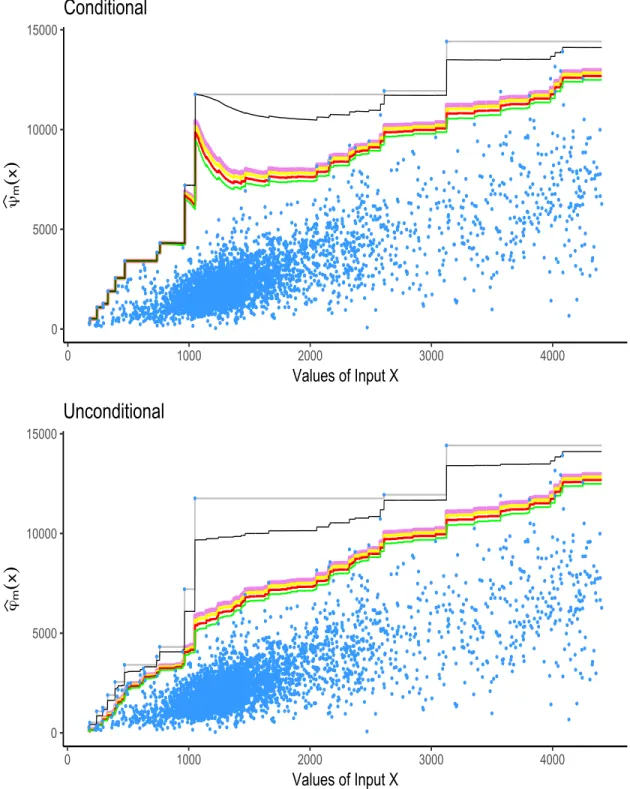
achieves the envelopment FDH surface ϕpxq as m Ñ 8. Top panels of Figure 1 and Figure 2p display, respectively, the scatterplots of our motivating real datasets on the activity of n “ 2, 326 and n “ 4, 000 delivery post offices, along with the estimated expected maximum production frontiers of order m “ 600, 700, 800, 900, n and m “ 8 (FDH). We refer readers to the online text for the coloured graphics.
The strength of the partial frontier estimators pψmpxq in terms of robustness has been established from a theoretical point of view by Daouia and Ruiz-Gazen (2006) and Daouia and Gijbels (2011). Yet, the conditioning by the event tX ď xu results in partial m-frontiers that can still be severely attracted by extreme and/or outlying observations with small Xi’s, especially as the input level x decreases. This is visualized in the top panels of Figure 1 and Figure 2, where the selected large m-frontiers pψmpxq coincide with the non-robust FDH estimator ϕpxq over an important range of values of x. Instead, we propose in the sequel top use a different formulation of expected maximum production functions without recourse to the conditioning by X ď x.
2.2
Robustified unconditional m-frontiers
For a fixed level of inputs-usage x P Rp` such that FXpxq ą 0, we propose to first transform the pp ` 1q-dimensional random vector pX, Y q and the n-tuple tpX1, Y1q, . . . , pXn, Ynqu into the dimensionless random variables
Yx“ Y 1IpX ď xq and Yix “ Yi1I pXi ď xq , i “ 1, . . . , n. (2) Their common distribution function FYxp¨q is closely related to the original conditional
dis-tribution function FY |Xp¨|xq since
FYxpyq “ 1 ´ FXpxqr1 ´ FY |Xpy|xqs( 1Ipy ě 0q.
A nice property of these transformed univariate random variables lies in the fact that ϕpxq ” supty ě 0 | FYxpyq ă 1u,
p
where pFYxpyq “ p1{nqřni“11IpYix ď yq. We then introduce the alternative concept of
ex-pected maximum achievable level of production ϕmpxq “ E“ maxpY1x, . . . , Ymxq‰ “
ż8
0
`1 ´ rFYxpyqsm˘ dy, (3)
where pYx
1 , . . . , Ymxq can be any m independent copies of Yx such as, for instance, the Yix’s described in (2). Clearly, for any trimming number m ě 1, the quantity ϕmpxq is nothing but the expectation of the FDH estimator based on the m-tuple tYx
i “ Yi1I pXi ď xqui“1,...,m. Of particular interest is the limiting case where the partial frontier function
ϕmpxq “ żϕpxq 0 `1 ´ rFYxpyqsm˘ dy “ ϕpxq ´ żϕpxq 0 rFYxpyqsmdy
converges monotonically to the true full frontier function ϕpxq as the trimming level m Ñ 8. Taking a closer look to ϕmpxq we see that it can be defined equivalently as the following special probability-weighted moments.
Proposition 1. For all m ě 1 and x P Rp` such that FXpxq ą 0, we have ϕmpxq ” E m ¨ rFYxpYxqsm´1¨ Yx ( ” E Jm`FY |XpY |xq ˘ ¨ Y |X ď x( , where Jm`FY |Xpy|xq ˘ “ mFXpxq“1 ´ FXpxqr1 ´ FY |Xpy|xqs ‰m´1 “ mPpX ď xq r1 ´ PpX ď x, Y ą yqsm´1.
The probability weight Jm`FY |Xpy|xq˘ assigns bigger weights to relevant outputs. Like ψmpxq, ϕmpxq achieves the optimal production frontier ϕpxq when the trimming number m tends to infinity. Likewise, its empirical version
p ϕmpxq “ ż8 0 `1 ´ r pFYxpyqsm˘ dy “ p ϕpxq ´ żϕpxqp 0 r pFYxpyqsmdy (4)
converges to the FDH frontierϕpxq as m Ñ 8. However, unlike pp ψmpxq, the weight-generating function defining ϕpmpxq is by construction appreciably less sensitive to border effects:
p ϕmpxq “ n ÿ i“1 Ypiqx "ˆ i n ˙m ´ˆ i ´ 1 n ˙m* (5)
where Ypiqx denotes the ith order statistic of the observations Y1x, . . . , Ynx. This marks a substantial difference with pψmpxq as can be visualized in the bottom panels of Figure 1 and Figure 2 for both cases of postal services.
2.3
Monotonicity requirement
From the point of view of the axiomatic foundation for production functions, nothing guar-antees that the usual conditional expected maximum production function ψmpxq and its estimator pψmpxq satisfy the monotonicity requirement. By contrast, both our population and sample unconditional versions ϕmpxq and ϕpmpxq enjoy the desirable axiom of mono-tonicity of the true efficient frontier ϕpxq. Indeed, it is not hard to verify that
FYxpyq ” t1 ´ PpX ď x, Y ą yqu 1Ipy ě 0q.
Then, for all y ě 0, the function x ÞÑ FYxpyq is nonincreasing. Therefore, the unconditional
partial frontier function ϕmpxq defined in (3) is nondecreasing in x, for all m ě 1. Likewise, it is easily seen that
p FYxpyq ” # 1 ´ 1 n n ÿ i“1 1IpXi ď x, Yi ą yq + 1Ipy ě 0q
is nonincreasing in x. Whence, the empirical estimator ϕpmpxq described in (4) is constrained to be nondecreasing in x, for all m ě 1. This advantage of the new class of unconditional expected maxima tϕpmu over the original concept of conditional versions t pψmu is better illustrated by Figure 2 (top versus bottom).
2.4
Asymptotic properties
From the asymptotic point of view, we first establish the following representation. Proposition 2. For all m ě 1 and all x P Rp` such that FXpxq ą 0, we have
?
ntϕpmpxq ´ ϕmpxqu “ ?
n Φm,npxq ` opp1q (6)
as n Ñ 8, where Φm,npxq “ mşϕpxq0 rFYxpyqsm´1
!
FYxpyq ´ pFYxpyq
) dy.
An immediate consequence of this result is that ?n ϕmpxq ´ ϕmpxq( is asymptoticallyp normal with zero mean and variance
σ2px, mq “ E #
m żϕpxq
0
rFYxpyqsm´1 1IpYx ď yq ´ FYxpyq(dy
+2 “ m2 żϕpxq 0 żϕpxq 0 “FYxpyqFYxpzq ‰m´1 FYxpy ^ zq ´ FYxpyqFYxpzq(dydz. (7)
8 10 12 14 4 6 8 Values of Input X ψm ( x )
Conditional
8 10 12 14 4 6 8 Values of Input X ϕm ( x )Unconditional
Figure 1: Scatterplot of the n “ 2, 326 delivery post offices (data in logarithms)— Estimated expected maximum production frontiers pψm (top) and ϕpm (bottom), with m “ 600, 700, 800, 900, n and m “ 8 (FDH), respectively, in green, red, yellow, violet, black and gray curves (see the online text for the coloured graphics).
0 5000 10000 15000 0 1000 2000 3000 4000 Values of Input X ψm ( x )
Conditional
0 5000 10000 15000 0 1000 2000 3000 4000 Values of Input X ϕm ( x )Unconditional
Figure 2: Scatterplot of the n “ 4, 000 delivery post offices—Estimated expected maximum production frontiers pψm (top) and ϕpm (bottom), with m “ 600, 700, 800, 900, n and m “ 8 (FDH), respectively, in green, red, yellow, violet, black and gray curves (see the online text for the coloured graphics).
Theorem 1. Suppose the support of Y is bounded. Then, for all m ě 1 and any X Ă Rp` such that infxPXFXpxq ą 0, (6) holds uniformly in x P X , that is
t?npϕmpxq ´ ϕmpxqq; x P X u “ tp ?
nΦm,npxq; x P X u ` opp1q, and ?npϕpm´ ϕmq converges in distribution in L
8pX q, as a process indexed by x P X , to the centered Gaussian process described in the proof.
Next, we show that ?n ϕpmpxq ´ ϕmpxq( also obeys a law of the iterated logarithm, which improves the order of convergence to Op?log log nq and even gives the proportionality constant.
Theorem 2. For all m ě 1 and x P Rp` such that FXpxq ą 0, we have almost surely, for either choice of sign,
lim sup nÑ8 ˘ ? n ϕpmpxq ´ ϕmpxq( p2 log log nq1{2 “ σpx, mq.
2.5
Robustness properties
From a robustness theory viewpoint, both the conditional expected maximum production function ψmpxq ” Tm,x`FpX,Y q˘ and its estimatorψpmpxq ” Tm,x
` p
FpX,Y q˘ are representable as a functional Tm,x of the population and empirical distribution functions
FpX,Y qpx, yq :“ PpX ď x, Y ď yq and FppX,Y qpx, yq :“ 1 n n ÿ i“1 1IpXi ď x, Yi ď yq, respectively, where the statistical functional Tm,x associates with a distribution function F p¨, ¨q on Rp`ˆ R`, such that F px, 8q ą 0, the real value
Tm,xpF q “ ż8 0 ˆ 1 ´„ F px, yq F px, 8q m˙ dy,
with the integrand being identically zero for y ě infty P R`|F px, yq{F px, 8q “ 1u. The rich-est quantitative robustness information is then provided by the influence function px0, y0q ÞÑ IF`px0, y0q; Tm,x, FpX,Y q˘ of Tm,x at FpX,Y q. It is defined as the first Gˆateaux derivative of the functional Tm,x at FpX,Y q, where the point px0, y0q plays the role of the coordinate in the infinite-dimensional space of probability distributions [see Hampel et al. (1986)]. The relevance of the influence function lies in its two main uses. First, it describes the effect of an infinitesimal contamination at the point px0, y0q on the estimate, standardized by the mass of the contamination. Second, it allows one to assess the relative influence of individual observations px0 “ Xi, y0 “ Yiq on the value of the estimate pψmpxq. An important robustness
requirement is the B-robustness [Rousseeuw (1981)] which corresponds to a finite gross-error sensitivity. The maximum absolute value
γ˚`Tm,x , FpX,Y q ˘ “ sup px0,y0qPRp`1` ˇ ˇIF ` px0, y0q; Tm,x, FpX,Y q ˘ |
defines the gross-error sensitivity of Tm,x at FpX,Y q. If this is unbounded, outliers can cause trouble. But according to Daouia and Ruiz-Gazen (2006), we have
IF`px0, y0q; Tm,x, FpX,Y q ˘ “ m FXpxq 1Ipx0 ď xq żϕpxq 0
FY |Xm´1py|xq“FY |Xpy|xq ´ 1Ipy0 ď yq‰ dy, (8) and hence γ˚`Tm,x, F
pX,Y q ˘
ď Fm
Xpxqϕpxq. Even more precisely, we show here the following.
Proposition 3. For all m ě 1 and x P Rp` such that FXpxq ą 0, γ˚`Tm,x, F pX,Y q ˘ “ m FXpxqmax # żϕpxq 0 FY |Xm py|xqdy, żϕpxq 0 FY |Xm´1py|xq“1 ´ FY |Xpy|xq‰ dy + ” m FXpxq max tϕpxq ´ ψmpxq, ψmpxq ´ ψm´1pxqu . (9)
The occurence of the vexing border effect of the partial frontier estimators pψmpxq, due to the conditioning by the event tX ď xu, is reflected by the presence of low values of FXpxq in the denominator of both (8) and (9).
Turning to the competing concept of unconditional expected maximum production func-tions, both ϕmpxq ” Tm`FYx˘ and
p
ϕmpxq ” Tm`FpYx˘ are representable as a functional Tm of
the population and empirical transformed distribution functions FYx and pFYx, respectively,
where Tm associates with a univariate distribution function F p¨q on R` the real value
TmpF q “ ż8 0 `1 ´ rF pyqsm˘dy “ żF´1p1q 0 `1 ´ rF pyqsm˘dy, with the integrand being identically zero for y ě F´1
p1q :“ infty P R|F pyq “ 1u. Following Hampel et al. (1986, Definition 1, p.84), the corresponding influence function of Tm at FYx
is defined as the ordinary derivative u P R` ÞÑ IF`u; Tm, FYx
˘
“ d
dt|t“0
Tmpp1 ´ tqFYx ` tδuq .
In robust statistics, a small fraction of the observations would have a strong influence on the estimator if their values were equal to a u where the influence function is large.
Proposition 4. For all m ě 1 and x P Rp` such that FXpxq ą 0, we have IF`u; Tm, FYx ˘ “ ´m żϕpxq 0
rFYxpyqsm´1 δupyq ´ FYxpyq(dy
” ´m żϕpxq
0
“1 ´ FXpxq ` FpX,Y qpx, yq‰m´1 1Ipu ď yq ´ 1 ` FXpxq ´ FpX,Y qpx, yq( dy. This closed form expression of the influence function indicates that the unconditional m-frontiers ϕpmpxq ” Tm`FpYx˘ do not suffer from the inherent border effects of the initial
concept of conditional m-frontiers pψmpxq ” Tm,x`FppX,Y q˘. Moreover, by making use of the same technique of the proof of Proposition 3, it is easily seen that the gross-error sensitivity λ˚`T m, FYx˘ :“ supuě0 ˇ ˇIF`u; Tm, FYx ˘ˇ ˇ satisfies λ˚`T m, FYx ˘ “ m ¨ max # żϕpxq 0 FYmxpyqdy, żϕpxq 0 FYm´1x pyq r1 ´ FYxpyqs dy + ” m ¨ max tϕpxq ´ ϕmpxq, ϕmpxq ´ ϕm´1pxqu which, in contrast to γ˚`Tm,x, F
pX,Y q˘, does not explode when x decreases. Also, as can be seen from (6) in Proposition 2, IF`Yx
i ; Tm, FYx˘ represents the approximate contribution, or
influence, of the observation pXi, Yiq toward the estimation error ϕpmpxq ´ ϕmpxq(, since ? ntϕpmpxq ´ ϕmpxqu “ ? n Φm,npxq ` opp1q ” ?1 n n ÿ i“1 IF`Yx i ; Tm, FYx ˘ ` opp1q, n Ñ 8.
Similarly, the influence function of the ‘conditional’ partial frontier estimator, described in (8), measures the asymptotic bias caused by contamination in the observations pXi, Yiq:
? n`ψmpxq ´ ψmpxqp ˘ “ ?1 n n ÿ i“1
IF`pXi, Yiq; Tm,x, FpX,Y q ˘
` opp1q, n Ñ 8.
However, the consideration of the ‘unconditional’ partial frontier estimator ϕpmpxq, instead of the conditional frontier estimator pψmpxq, may result in a better asymptotic variance (7), especially when PpX ď xq is small.
2.6
Regularized frontier estimators
It should be clear that the estimation of a “partial” frontier ϕm, for a sufficiently large value of m, instead of the “full” frontier ϕ is mainly motivated by the search for a “robust” frontier estimator ϕpm which is well inside the cloud of data points tpXi, Yiq, i “ 1, . . . , nu, but lies near the true upper support boundary. The robustness of ϕpm comes from its convergence monotonely from below to the smallest sample envelope (FDH) ϕ as the trimming numberp
m increases. When m “ mnÑ 8 at a fast rate as n Ñ 8, the next theorem shows that the robust frontier ϕpmnpxq estimates ϕpxq itself and converges to the same limit distribution as
the FDH estimator ϕ with the same scaling. Recall first that, following Daouia et al. (2010,p Theorem 2.1), there exists bn ą 0 such that b´1n pϕpxq ´ ϕpxqq converges to a non-degeneratep distribution if and only if
FXpxqr1 ´ FY |Xpy|xqs “ Lx `
tϕpxq ´ yu´1˘pϕpxq ´ yqρx as y Ò ϕpxq,
for some constant ρx ą 0, where Lxp¨q is a slowly varying function, that is, limtÒ8Lxptzq{Lxptq “ 1 for all z ą 0. The limit distribution function is identical to
Fρxpyq “ expt´p´yq
ρx
u with support p´8, 0s.
Under the sufficient condition that Lxptϕpxq ´ yu´1q „ `x ą 0 as y Ò ϕpxq, that is Condition Cpρx, `xq: For some constants ρx ą 0 and `x ą 0,
FXpxqr1 ´ FY |Xpy|xqs “ `x`ϕpxq ´ y˘ ρx
` o`pϕpxq ´ yqρx˘ as y Ò ϕpxq,
it is shown in Daouia et al. (2010, Corollary 2.1) that bn „ pn`xq´1{ρx and pn`xq1{ρx ϕpxq ´
p
ϕpxq( ÝÑ Weibullp1, ρxqL as n Ñ 8,
where a random variable W is said to follow the distribution Weibullp1, ρxq if Wρx is
Expo-nential with parameter 1. As described thoroughly in Remark 2.3 of Daouia et al. (2010), the exponent ρx has the following intuitive meaning in terms of the density of pX, Y q and the dimension pp ` 1q: When ρxą p ` 1, the joint density decays to zero at a speed of power ρx´ pp ` 1q of the distance from the frontier point ϕpxq. When ρx “ p ` 1, the density has a sudden jump at the frontier. Finally, when ρx ă p ` 1, the density rises up to infinity at a speed of power ρx´ pp ` 1q of the distance from the frontier.
Theorem 3. For x P Rp` such that FXpxq ą 0, if Cpρx, `xq holds and mn ě βn log nt1 ` op1qu for some constant β ą ρ1
x ` 1, then pn`xq1{ρx ϕpxq ´ p ϕmnpxq ( L ÝÑ Weibullp1, ρxq as n Ñ 8.
By contrast, when m “ mnÑ 8 at a slow rate as n Ñ 8, the robust frontier estimator p
ϕmnpxq becomes asymptotically Gaussian, as in the regular case of a fixed m.
Theorem 4. Let x P Rp` such that FXpxq ą 0. (i) If mn Ñ 8 and m 2 n σpx,mnq “ O ´ ? n log log n ¯ as n Ñ 8, then ? n σpx, mnqtϕpmnpxq ´ ϕmnpxqu L ÝÑ N p0, 1q, n Ñ 8. (10)
(ii) Under the extreme-value condition Cpρx, `xq , we have
cxm1´2{ρx ď σ2px, mq ď ˜cxm2´2{ρx as m Ñ 8, for some positive constants cx and ˜cx.
(iii) Also, under Cpρx, `xq , if mnÑ 8 with mn “ O
´ ?
n log log n
¯3 1
2 `ρx1 , then the asymptotic
normality (10) is still valid.
Note that the explicit condition mn Ñ 8 with mn “ O
´ ?
n log log n
¯3 1
2 `ρx1 , in Theorem 4 (iii),
implies that mn{?n Ñ 0 as n Ñ 8. We would like also to comment on the speed of convergence ?n{σpx, mnq, obtained in Theorem 4 (i) and (iii), when the trimming level mn Ñ 8 at a slow rate so that mn “ c
´ ?
n log log n
¯3 1
2 `ρx1 , for some constant c ą 0. By
Theorem 4 (ii), as n Ñ 8, we get k1 ? n 1 2 `ρx2 3 2 `ρx1 plog log nq 1´ 1ρx 3 2 `ρx1 ď ? n σpx, mnq ď k2 ? n 1` 2ρx 3 2 `ρx1 plog log nq 1 2 ´ρx1 3 2 `ρx1
for some constants k1, k2 ą 0. In the particular case ρx “ p ` 1, often assumed in the literature of production econometrics, which corresponds to a joint density of pX, Y q having a jump at the frontier point ϕpxq, we have
k1`n3{2log log n ˘1{4 ď ? n σpx, mnq ď k2 ? n as p “ 1,
and k1n1{6plog log nq 2{3 ď ? n σpx, mnq ď k2pn log log nq 1{3 as p Ò 8.
Interestingly, even when the data dimension explodes, the speed of convergence does not deteriorate too much, thereby reducing the curse of dimensionality that is typical of many nonparametric frontier estimators such us, for instance, the FDH estimator.
2.7
Bias-corrected estimator of ϕpxq
Under the extremal condition Cpρx, `xq , when mn Ñ 8 with mn “ O
´ ?
n log log n
¯3 1
2 `ρx1 ,
Theorem 4 (iii) actually indicates that ϕpmnpxq estimates ϕpxq itself with the inherent bias
Bmnpxq “ ϕpxq ´ ϕmnpxq such that ? n σpx, mnqtϕpmnpxq ´ ϕpxq ` Bmnpxqu L ÝÑ N p0, 1q, n Ñ 8. (11)
Recall that, in view of (3),
ϕmnpxq “ E“ maxpY x 1 , . . . , Y x mnq ‰
is nothing but the expectation of the FDH estimator, maxpYx
1, . . . , Ymxnq ” maxi:XiďxYi,
based on the mn-tuple tYx
i “ Yi1I pXi ď xqui“1,...,mn. Under the sufficient condition Cpρx, `xq,
the limit theorem of moments of the FDH estimator in Daouia et al. (2010, Theorem 2.1 (iii)) shows that lim mnÑ8E“b ´1 mn ϕpxq ´ maxpY x 1, . . . , Y x mnq (‰ “ Γp1 ` 1{ρxq, where Γ is the gamma function, which entails that
lim mnÑ8 b´1 mntϕpxq ´ ϕmnpxqu “ Γp1 ` 1{ρxq, (12) with bmn „ pmn`xq ´1{ρx, or equivalently, Bmnpxq “ ϕpxq ´ ϕmnpxq “ pmn`xq ´1{ρxΓp1 ` 1{ρxq ` o`m´1{ρx n ˘ , n Ñ 8. (13)
Combining this with Theorem 4 (ii), it follows that the introduced bias (normalized by the rate of convergence) is bounded below by
? n σpx, mnqBmnpxq ą ˇcx ´? n 1 2` 1 ρx log log n ¯3 1 2 `ρx1 ,
for some constant ˇcx ą 0. The normalized bias does not then vanish asymptotically, and hence one would use in practice the asymptotic approximation:
ϕpxq ´ϕpmnpxq « N ˆ Bmnpxq, σ2px, mnq n ˙ , where Bmnpxq and σ 2
px, mnq have to be replaced by consistent estimators. The plugging version of σ2px, mnq in (7) provides a consistent estimator of this asymptotic variance. As for the bias term, a consistent estimator can be obtained through the leading part of (13) once ρx and `x are consistently estimated. One way of estimating these parameters is by adapting the ideas from Section 4.1 in Daouia et al. (2012). Given an integer a ě 2, we have by (12) that lim nÑ8 ϕamnpxq ´ ϕmnpxq ϕa2m npxq ´ ϕamnpxq “ a1{ρx,
which motivates the estimator
p ρx :“ logpaq " log ˆ p ϕamnpxq ´ϕpmnpxq p ϕa2m npxq ´ϕpamnpxq ˙*´1 . (14)
On the other hand, it follows from (13) that `x „ 1 mn „ p1 ´ a´1{ρxqΓp1 ` 1{ρxq ϕamnpxq ´ ϕmnpxq ρx , n Ñ 8,
which suggests the estimator p `x :“ 1 mn „ p1 ´ a´1{ρpxqΓp1 ` 1{pρxq p ϕamnpxq ´ϕpmnpxq pρx . (15)
Both ρxp and p`x are consistent estimators.
Theorem 5. Under the conditions of Theorem 4 (iii),
p ρx p ÝÑ ρx and p`x p ÝÑ `x as n Ñ 8. (16)
Let us now return to the starting point (4.3) to investigate the asymptotic normality of the bias-corrected estimator itself. This estimator is defined as
r
ϕmnpxq :“ϕpmnpxq ` pBmnpxq, (17)
where, assuming for ease of presentation that ρx is given, p
Bmnpxq :“ pmn`pxq
´1{ρxΓp1 ` 1{ρxq
is the plug-in version of the bias Bmnpxq obtained by replacing `x, in the leading part of (13),
with its consistent estimate
p `x :“ p`xp ˜mnq “ 1 ˜ mn „ p1 ´ a´1{ρxqΓp1 ` 1{ρxq p ϕa ˜mnpxq ´ϕpm˜npxq ρx . (18)
Here, we shall distinguish between the trimming level mn in the estimator ϕmr npxq of the
frontier function ϕpxq and the level ˜mnused in the estimator p`xof the parameter `x. Nothing guarantees that the two levels are necessarily the same. It should also be noted that, while the asymptotic normality of the partial frontier estimator ϕpmnpxq in Theorem 4 hinges on
the first-order representation (13), that is ϕpxq ´ ϕmnpxq “ pmn`xq
´1{ρxΓp1 ` 1{ρxq ` o`m´1{ρx
n ˘ , n Ñ 8,
which is implied by the extremal condition Cpρx, `xq, the asymptotic normality of the full frontier estimator ϕrmnpxq requires the following second-order representation:
Condition C2pρx, `x, αxq: For some constants ρx ą 0, `x ą 0 and αx ą 0, ϕpxq ´ ϕmnpxq “ pmn`xq
´1{ρxΓp1 ` 1{ρxq ` o`m´p1`αxq{ρx
n ˘ , n Ñ 8,
where the extra parameter αx is needed to control the speed of convergence, in the first-order condition, of pmn`xq1{ρxtϕpxq ´ ϕm
Theorem 6. Let x P Rp` such that FXpxq ą 0. Under Cpρx, `xq and C2pρx, `x, αxq with αxą ρx`1, if mn “ c ´ ? n log log n ¯3 1 2 `ρx1 ´ε and ˜mn“ ˜c ´ ? n log log n ¯3 1 2 `ρx1 ´˜ε
, for some constants c, ˜c ą 0 and 0 ă ˜ε ă ´ 3 2 ` 1 ρx ¯´1 ă 2˜ε ´ ε, such that 1 ´12 ˆ 1 3 2` 1 ρx ´ ε ˙ ´αx ρx ˆ 1 3 2` 1 ρx ´ ˜ ε ˙ ă 0, then ? n σpx, mnq ` r ϕmnpxq ´ ϕpxq ˘ L ÝÑ N p0, 1q as n Ñ 8.
The condition αx ą ρx ` 1 in Theorem 6 is needed to control the bias approximation error (driven by the last term in C2pρx, `x, αxq) so as to get
? n σpx,mnqo ´ m´p1`αxq{ρx n ¯ “ op1q. The condition ´ 3 2 ` 1 ρx ¯´1 ă 2˜ε ´ ε is required to select mrn “ o ´ m1{2n ¯ in the estimator p
`x :“ p`xp ˜mnq of `x. It is easily seen that the condition ˜ε ă ´ 3 2 ` 1 ρx ¯´1 implies 1 ´ 1 2 ˜ 1 3 2 ` 1 ρx ´ ε ¸ ´αx ρx ˜ 1 3 2 ` 1 ρx ´ ˜ε ¸ ă 1 ´ 1 2p˜ε ´ εq. Hence, the last condition of the theorem, that is 1 ´ 12
ˆ 1 3 2` 1 ρx ´ ε ˙ ´αx ρx ˆ 1 3 2` 1 ρx ´ ˜ ε ˙ ă 0 is satisfied if, for instance, ˜ε ´ ε ą 2.
It should be noted that we restrict ourselves in Theorem 6 to the case where ρx is known. This corresponds, for instance, to the standard assumption in productivity and efficiency analysis that the joint density of data pXi, Yiq has jumps at the frontier, or equivalently ρx “ p ` 1 (see the discussion above Theorem 3). The question of whether the asymptotic normality in Theorem 6 still holds when replacing ρx by its estimator ρpx is of interest. The complexity of using ρpx in place of ρx in the proof is that it adds two additional terms to the two terms I and II already in use in (A.8). Theoretical developments along these lines are left for future research.
3
Trimming selection problem
We return here to our real data examples with a single input (p “ 1) to explore in Section 3.1 the selection of the trimming level mn in the partial frontierϕpmn, before moving to the final
bias-corrected frontier ϕrmnpxq in Section 3.2. We extend our discussion to multiple inputs
(p ą 1) in Section 3.3.
3.1
Selecting the partial frontier
ϕ
p
mnIn productivity and efficiency analysis where outliers are likely to affect traditional envelop-ment approaches, a common robust practice in operations research and applied work consists
in using an empirical partial frontier as a benchmark to measure the efficiency of production units. Unfortunately, the chosen partial frontier is often based on an a priori selected order m “ mn in the case of conditional expected maxima, or tail probability in the case of con-ditional quantiles. Here, we propose practical guidelines for a more justified selection from a robustness theory viewpoint.
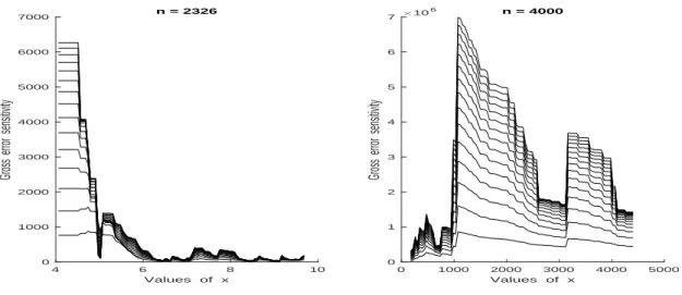
As with any trimming techniques, the degree of truncation, here reflected through m selection, is a major issue in practice. But monotonicity itself is a rather powerful way of regularizing the estimated expected maximum production function. Because it elimi-nates sharp changes in the slope and curvature of the unconditional m-frontier function, the trimming selection problem tends to be easier than unconstrained conditional m-frontier estimation. Of course, if the model is known or believed to be nearly correct, then the use of the envelopment FDH estimator pm “ 8q is required. Otherwise, if the dataset contains suspicious isolated extreme observations, it is more prudent to seek for ‘robustification’ via the choice of an adequate trimming level m. To verify the presence of such influential obser-vations among the data (e.g. French and European postal datasets), a simple diagnostic tool is by using the gross-error sensitivity of the sequence tϕpmum which corresponds to the maxi-mum influence function. Figure 3 shows the sample gross-error sensitivity x ÞÑ λ˚`Tm, pF
Yx˘,
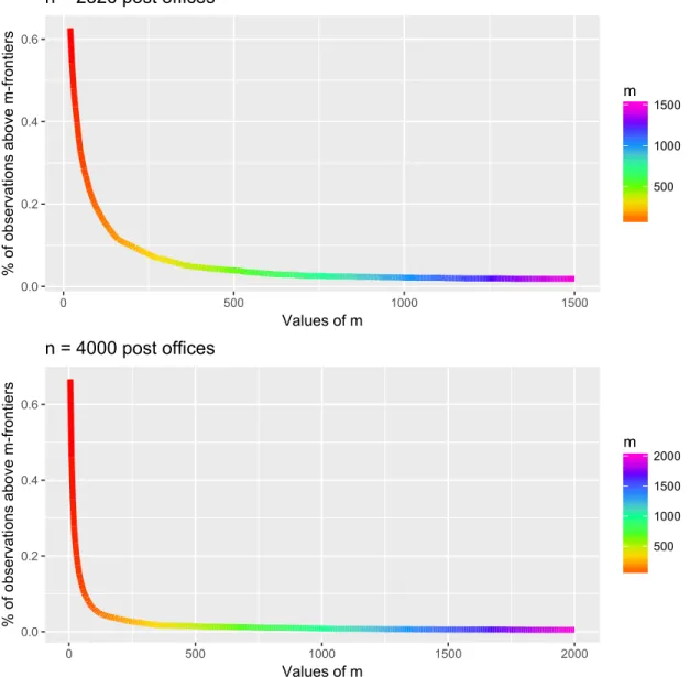
for various values of m “ 100, 200, . . . , 1500. For both postal services, the evolution of λ˚ exhibits some slight and severe breakdowns at different values of x, especially in the case of French post offices (r-h.s). This indicates the presence of isolated extreme and/or anomalous data. One way of choosing the trimming number m is then by looking to Figure 4 which indicates how the percentage of data points pXi, Yiq above the curve ofϕpmdecreases with m. The basic idea is to choose values of m for which the frontier estimatorϕpm is sensitive to the magnitude of valuable extreme post offices while remaining resistant to isolated outliers.
The evolution of the percentage in both sectors of Delivery Services has clearly an “L” structure highlighted by a colour-scheme, ranging from dark red (high %) to dark violet (low %). We refer readers to the online text for the “colouring of the L evolution”. Such an L deviation should appear for any other analyzed data set since, by construction, the probability-weighted moments ϕpm steer an advantageous middle course between sensitivity and robustness to extreme values and/or outliers. In the case of 2, 326 delivery post offices (top picture in Figure 4), the percentage first falls rapidly along the ‘red’ part of the curve. This means that most of the observations lying above the corresponding m-frontiers are not extremes but interior points to the cloud of data points. Then the evolution of the percentage shows an “elbow effect” along the ‘orange’ and ‘green’ parts of the curve. This means that the observations outside the corresponding m-frontiers are no more inefficient, but still contain either relatively efficient post offices that are well inside the sample or top
4 6 8 10 Values of x 0 1000 2000 3000 4000 5000 6000 7000
Gross error sensitivity
n = 2326 0 1000 2000 3000 4000 5000 Values of x 0 1 2 3 4 5 6 7
Gross error sensitivity
106 n = 4000
Figure 3: Plots of x ÞÑ λ˚`Tm, pFY
x˘ for m “ 100, 200, . . . , 1500. From left to right, the 2,326
and 4,000 post offices.
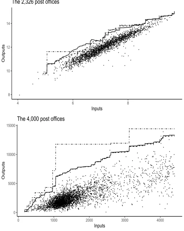
observations that are valuable post offices. In contrast, after the elbow effect, it may be seen that the percentage decreases very slowly along the ‘blue’ part, say 850 ď m ď 1250, before becoming extremely stable along the ‘violet’ part of the curve. This means that all observations left outside the partial frontier of order m “ 850 are really very extreme in the Y -direction and could be outlying or perturbed by noise. This might suggest to select 850 as a potential lower value for m. On the other hand, the extreme stability of the percentage curve from m “ 1250 may indicate that the observations above the frontier ϕp1250 are really outlying or suspicious isolated extremes that deserve to be carefully examined. This might suggest to choose 1250 as a potential upper value for m. The two potential choices of the frontier estimator ϕpm are graphed in Figure 5 along with the FDH estimator.
As regards the 4, 000 delivery post offices (bottom picture in Figure 4), it may be seen that the “elbow effect” corresponds to the ‘orange’ part of the percentage curve, and the desired range of values of m follows as the ‘green’ part, say, 500 ď m ď 1000. The lower and upper selected prudential frontiers ϕ500p and ϕ1000p are superimposed in Figure 5 along with the FDH estimator. Unsurprisingly, there are very few observations lying between the two partial frontiers.
0.0 0.2 0.4 0.6 0 500 1000 1500 Values of m % o f o bse rva tio ns ab ove m-f ro nt ie rs 500 1000 1500 m n = 2326 post offices 0.0 0.2 0.4 0.6 0 500 1000 1500 2000 Values of m % o f o bse rva tio ns ab ove m-f ro nt ie rs 500 1000 1500 2000 m n = 4000 post offices
Figure 4: Evolution of the % of sample points outside the partial m-frontiers ϕpm (see the online text for a colour-scheme).
3.2
The final bias-corrected frontier
ϕ
r
mnpxq
Under the usual assumption in production econometrics that ρx “ p`1 ” 2, the final frontier estimator ϕrmnpxq has the closed form expression
r ϕmnpxq “ ϕrmn, ˜mn,apxq “ ϕpmnpxq ` pmn`pxq ´1{ρxΓp1 ` 1{ρxq ” ϕpmnpxq ` ˆ ˜mn mn ˙1{2 p ϕa ˜mnpxq ´ϕpm˜npxq p1 ´ a´1{2q ,
8 10 12 14 4 6 8 Inputs Outputs
The 2,326 post offices
0 5000 10000 15000 0 1000 2000 3000 4000 Inputs Outputs
The 4,000 post offices
Figure 5: Selected (lower and upper) expected maximum production frontiers ϕm. Top—p dataset of size 2, 326 in logarithms, with m “ 1250 (upper) in solid line, m “ 850 (lower) in dashed line, and m “ 8 (FDH) in dashdotted line. Bottom—dataset of size 4, 000, with m “ 1000 (upper) in solid line, m “ 500 (lower) in dashed line, and m “ 8 (FDH) in dashdotted line.
where mn P r850, 1250s for the sample size 2,326 and mn P r500, 1000s for the sample size 4,000. For illustration purposes, we restrict to the upper selected prudential levels mn“ 1250 for n “ 2,326 and mn “ 1000 for n “ 4,000. Our experience with these data indicates that
r
ϕmnpxq is not sensitive to the choice of the tuning parameter a ě 2. For example, the
frontier estimates obtained for all values of a in r2, 10s appear to be very similar. However, the estimates seem to be more sensitive to the choice of ˜mn. This is illustrated in Figure 6 for both datasets, where the final bias-corrected frontiers x ÞÑϕrmnpxq are plotted for a “ 2
and two different values of ˜mn “ m0.005n (dashed) and ˜mn “ m0.2n (solid), along with the non-robust FDH frontier (dashdotted). Although the resulting (blue and red) frontiers for both values of ˜mn are very close for the largest dataset of size n “ 4,000 (bottom panel), it may be seen that they are quite different in the case n “ 2,326 (top panel). We do not enter here into the question of optimal selection of ˜mn, but it is clearly of genuine interest and is still open for future research.
3.3
Extension to multiple inputs
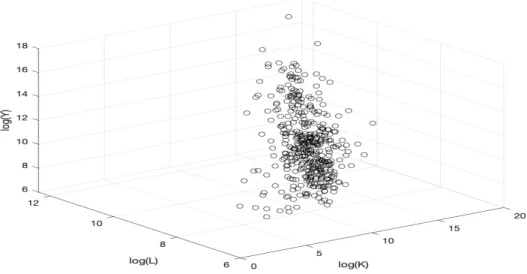
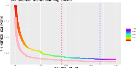
It should be clear that, thanks to the dimensionless transformation adopted in (2), the practical guidelines described above evidently apply to higher dimension p ą 1. For our illustration purposes we consider here a real data example in the case p “ 2, where the dataset consists of n “ 406 firms in the petroleum, chemical and plastics industries in Ecuador in 2002. For each firm, we have information on the capital K in thousands of USD, the average number of employees L and the value-added real output Y in thousands of USD. The scatterplot of the 406 observations (in logarithm scale) is displayed in Figure 7. In this particular example, the efficient FDH surface is determined by only 12.56% of the firms, and some of these extremal FDH firms are outlying as can be seen from Daouia and Park (2013). The latter authors used the ‘conditional’ partial m´frontiers t pψmum, rather than the unreliable FDH frontier, as a robust benchmark for the assessment of the production performance of firms. The objective here is to compare their method with our alternative proposal of ‘unconditional’ partial m´frontiers tϕmum, for a suitable choice of the trimmingp levels m.
Figure 8 shows the evolution of the percentage of sample points left outside both partial m-frontiers pψm (pink curve) and ϕpm (rainbow curve); we refer readers to the online text for the coloured graphics. The decrease of the percentage corresponding to the ‘uncondi-tional’ partial m-frontiersϕpm is clearly slower than the one corresponding to the ‘conditional’ versions pψm. This reflects the resistance of the ‘unconditional’ partial m-frontiers to the mag-nitude of extremes and/or outliers. It may also be seen that the decrease of the percentage
8 10 12 14 4 6 8 Inputs Outputs
The 2,326 post offices
0 5000 10000 15000 0 1000 2000 3000 4000 Inputs Outputs
The 4,000 post offices
Figure 6: Final bias-corrected frontiers x ÞÑ ϕrmn, ˜mn,apxq for a “ 2 and two different values
of ˜mn “ m0.005n (dashed) and ˜mn “ m0.2n (solid), along with the FDH frontier (dashdotted). Top—dataset of size 2,326 in logarithms, with mn “ 1250. Bottom—dataset of size 4,000, with mn“ 1000.
Figure 7: The capital K (in log), the average number of employees L (in log) and the value-added real output Y (in log).
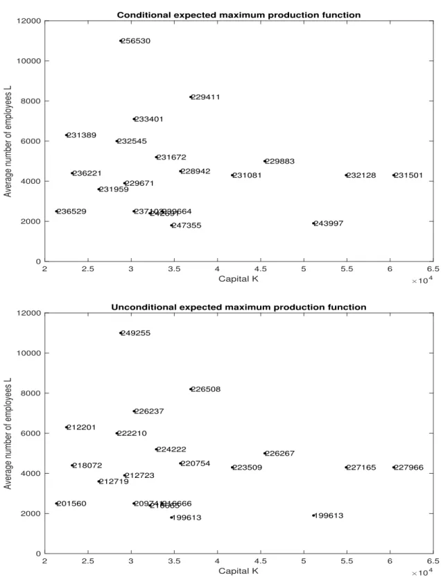
becomes very slow from m “ 183 for the pink curve (indicated by the vertical pink line) and from m “ 336 for the rainbow curve (indicated by the vertical blue line). Figure 9 (top panel) shows the resulting values pψ183pxiq for 20 randomly chosen grid inputs xi “ pKi, Liq. As is to be expected in the case of conditional expected maxima, there are many violations of monotonicity by the multi-argument function pψ183pxiq (with respect to the partial order induced by ‘ď’). Figure 9 (bottom panel) displays the values of ϕp336pxiq for the same se-lected 20 points, showing that the unconditional expected maximum production function is well isotonic nondecreasing. When taking larger trimming levels m (in the stable regions starting from the vertical dashed lines), the lessons were the same in terms of robustness and monotonicity.
4
Numerical illustrations
In this section, we illustrate our procedure through two standard examples with simulated data. We consider the same data generating processes traditionally used in the literature of nonparametric frontier estimation such as, for instance, Gijbels et al. (1999), Cazals et al. (2002), Simar (2003), Florens and Simar (2005), Daouia et al. (2005), Daouia and Ruiz-Gazen (2006), Daouia and Gijbels (2011), and Noh (2014).
Example 1. We first consider a situation where the upper extremity of the joint support of pX, Y q is linear. We choose pX, Y q uniformly distributed over the triangle tpx, yq P r0, 1s2 :
0.25 0.50 0.75 1.00 0 100 200 300 400 Values of m % of ob serva tion s a bove m-f ron tiers 100 200 300 400 m Ecuadorian manufacturing sector
Figure 8: Evolution of the % of sample points outside the partial m-frontiers pψm (pink) and ϕpm (rainbow), see the online text for the coloured graphics. The vertical dashed lines correspond to m “ 183 (pink) and m “ 336 (blue).
y ď xu. Here, the true full frontier function is ϕpxq “ x, and the conditional distribution function is FY |Xpy|xq “ 2x´1y ´ x´2y2, for 0 ă x ď 1 and 0 ď y ď ϕpxq. The partial conditional order-m frontier function is
ψmpxq “ ϕpxq ´ m ÿ k“0 ˆm k ˙ 2m´kp´1qkx{pm ` k ` 1q. Its unconditional analogue for the same order m is given by
ϕmpxq “ ϕpxq ´ m ÿ k“0 ˆm k ˙ p´1qkx2k`1{p2k ` 1q.
Example 2. We now consider a more realistic example from the point of view of production econometrics. We choose a non-linear production frontier given by the Cobb-Douglas model Y “ X1{2expp´U q, where X is uniform on r0, 1s and U , independent of X, is exponential with mean 1{3. Here, the full production function is ϕpxq “ x1{2, and the conditional distribution function is FY |Xpy|xq “ 3x´1y2´ 2x´3{2y3, for 0 ă x ď 1 and 0 ď y ď ϕpxq. The partial order-m frontier functions have the following closed form expressions:
ψmpxq “ ϕpxq ´ m ÿ k“0 ˆm k ˙ 3m´kp´2qk?x{p2m ` k ` 1q, ϕmpxq “ ϕpxq ´ m ÿ k“0 ˆm k ˙ xk`1{2p´1qk k ÿ j“0 ˆk j ˙ j ÿ i“0 ˆj i ˙ p´3qj´i2i{p2j ` i ` 1q.
2 2.5 3 3.5 4 4.5 5 5.5 6 6.5 Capital K 104 0 2000 4000 6000 8000 10000 12000
Average number of employees L
Conditional expected maximum production function
243997 231959 229883 231501 231672 242691 231081 247355 237103 236529 239664 231389 229671 232545 233401 236221 232128 229411 256530 228942 2 2.5 3 3.5 4 4.5 5 5.5 6 6.5 Capital K 104 0 2000 4000 6000 8000 10000 12000
Average number of employees L
Unconditional expected maximum production function
199613 212719 226267 227966 224222 216665 223509 199613 209741 201560 216666 212201 212723 222210 226237 218072 227165 226508 249255 220754
Figure 9: In both pictures, the points indicate 20 randomly chosen grid inputs xi “ pKi, Liq. The number associated to each point xi indicates the conditional expected maximum pψ183pxiq (top) and the unconditional expected maximum ϕ336pxip q (bottom).
4.1
Comparison of population m´frontiers
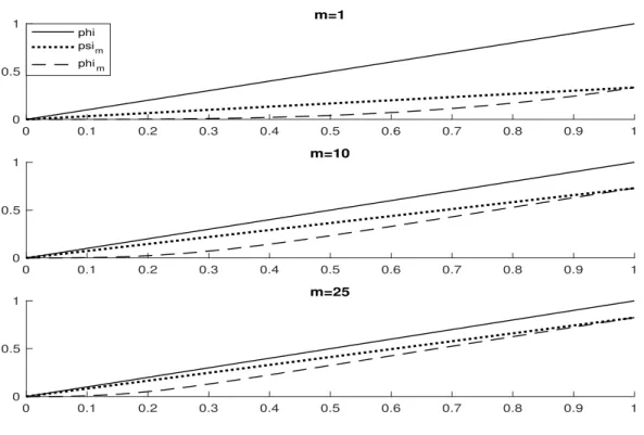
For both examples, the graphs of ψm and ϕm are superimposed in Figures 10 and 11, for three values of m “ 1, 10, 25, along with the true support boundary ϕ. First, it may be seen from the plots that the conditional m´frontiers ψmpxq [dotted curves] diverge from the true frontier ϕpxq [solid curve] as x increases. Whereas the new unconditional m´frontiers ϕmpxq [dashed curves] tend to be more parallel to the full frontier ϕpxq. Second, the partial condi-tional m´frontiers approach rapidly the full frontier as m increases, while the convergence of the unconditional m´frontiers seems to be slower. Already these substantial differences indicate the usefulness of the new concept of unconditional expected maximum production m´frontiers.
Moreover, the new unconditional m´frontier ϕm can be viewed as a ‘robustified’ alter-native to the original conditional m´frontier ψm, for each trimming level m. This is visu-alised in Figures 12 and 13, where the gross-error sensitivities γ˚`Tm,x, FpX,Y q˘ of ψmpxq and λ˚`T
m, FYx˘ of ϕmpxq are plotted against m, for various values of x P t1
4, 1 2,
3
4u. According to Hampel, Ronchetti, Rousseeuw and Stahel (1986, p.43), the most important quantita-tive robustness requirement is a low gross-error sensitivity. From this basis, it is clear that the new class of unconditional m´frontiers affords more reliability since the corresponding gross-error sensitivity λ˚ [dashed line] is overall smaller than γ˚ [solid line]. Of interest is the limit case m Õ 8, where γ˚ explodes especially for low inputs-usage x, whereas λ˚ remains appreciably small and stable whatever the value of x. This indicates that the se-quence of empirical unconditional m´frontiers tϕmpxqunp is more resistant to extreme values and/or outliers than its conditional analogue t pψmpxqun for estimating the true full frontier ϕpxq “ limmÑ8ϕmpxq “ limmÑ8ψmpxq. The lack of robustness of t pψmpxqun, for small values of x, is due to its construction via the conditioning by X ď x.
4.2
Biased frontier estimators
To evaluate finite-sample performance of pψmp¨q and ϕpmp¨q, as robust estimators of ϕp¨q, we have undertaken some simulation experiments. All the experiments were performed over 1,000 simulations for the sample sizes n “ 100, 500, 1000. Three outliers were added in each simulated data set: tp0.1, 0.6q, p0.35, 0.8q, p0.6, 1qu for both uniform-triangle and Cobb-Douglas examples. The measures of efficiency for each simulation used were the mean squared
0 0.1 0.2 0.3 0.4 0.5 0.6 0.7 0.8 0.9 1 0 0.5 1 m=1 phi psim phim 0 0.1 0.2 0.3 0.4 0.5 0.6 0.7 0.8 0.9 1 0 0.5 1 m=10 0 0.1 0.2 0.3 0.4 0.5 0.6 0.7 0.8 0.9 1 0 0.5 1 m=25
Figure 10: Uniform triangle example—Graphs of ϕ in solid line, ψm in dotted line, and ϕm in dashed line. 0 0.1 0.2 0.3 0.4 0.5 0.6 0.7 0.8 0.9 1 0 0.5 1 m=1 phi psim phim 0 0.1 0.2 0.3 0.4 0.5 0.6 0.7 0.8 0.9 1 0 0.5 1 m=10 0 0.1 0.2 0.3 0.4 0.5 0.6 0.7 0.8 0.9 1 0 0.5 1 m=25
0 10 20 0 2 4 6 8 10 12 14 16
Gross error sensitivity
x = 1/4 gamma* lambda* 0 10 20 m 0 2 4 6 8 10 12 14 16 x = 1/2 0 10 20 0 2 4 6 8 10 12 14 16 x = 3/4
Figure 12: Uniform triangle example—Gross-error sensitivities m ÞÑ γ˚`Tm,x, F pX,Y q
˘ in solid line and m ÞÑ λ˚`T
m, FYx˘ in dashed line. 0 10 20 0 0.5 1 1.5 2 2.5 3 3.5 4 4.5 5
Gross error sensitivity
x = 1/4 gamma* lambda* 0 10 20 m 0 0.5 1 1.5 2 2.5 3 3.5 4 4.5 5 x = 1/2 0 10 20 0 0.5 1 1.5 2 2.5 3 3.5 4 4.5 5 x = 3/4
Figure 13: Cobb-Douglas example—Gross-error sensitivities plots as before.
error and the bias MSEt pψmu “ 1 L L ÿ `“1 ! p ψmpx`q ´ ϕpx`q )2 , Biast pψmu “ 1 L L ÿ `“1 ! p ψmpx`q ´ ϕpx`q ) MSEtϕpmu “ 1 L L ÿ `“1 tϕpmpx`q ´ ϕpx`qu 2 , Biastϕpmu “ 1 L L ÿ `“1 tϕpmpx`q ´ ϕpx`qu
with the x`’s being L “ 100 points regularly distributed in r^Xi, _Xis. To guarantee a fair comparison among the two rival estimation methods, we used for each estimator the optimal parameter m minimizing its MSE over the wide range t1, . . . , nu. The resulting values of
MSE and bias are averaged on the 1,000 Monte Carlo replications and reported in Tables 1 and 2, along with the average m of the optimal 1,000 trimming levels m. The obtained estimates provide Monte Carlo evidence that the new class of partial m´frontiers tϕpmum is more efficient and robust relative to t pψmum for estimating ϕ. A typical realization of the experiment in each simulated scenario with n “ 100 is shown in Figure 14, where the optimal parameter m of each frontier estimator was chosen in such a way to minimize its MSE.
MSE n t pψmu tϕpmu 100 0.0414 0.0031 500 0.0240 0.0014 1000 0.0175 0.0010 Bias t pψmu tϕpmu 0.0169 -0.0103 -0.0219 -0.0104 -0.0312 -0.0095 m t pψmu tϕpmu 7.90 31.76 15.71 100.61 21.02 163.09
Table 1: Uniform triangle example—Results averaged on 1,000 simulations.
MSE n t pψmu tϕpmu 100 0.0050 0.0019 500 0.0023 0.0006 1000 0.0016 0.0004 Bias t pψmu tϕpmu -0.0104 -0.0101 -0.0147 -0.0074 -0.0139 -0.0062 m t pψmu tϕpmu 21.19 51.24 51.42 150.73 76.65 239.33
Table 2: Cobb-Douglas example—Results averaged on 1,000 simulations.
4.3
Bias-corrected frontier estimators
This section provides Monte Carlo evidence on the usefulness of the proposed ‘unconditional’ expected maximum output frontiers relative to their ‘conditional’ competitors in terms of average lengths and achieved coverages of the corresponding asymptotic confidence intervals. More specifically, Theorem 4 indicates that ϕpmpxq estimates ϕpxq itself with the inherent bias Bmpxq “ ϕpxq ´ ϕmpxq such that
? n
σpx, mqtϕpmpxq ´ ϕpxq ` Bmpxqu L
ÝÑ N p0, 1q, n Ñ 8,
for a suitable choice of m “ mnÑ 8 as n Ñ 8. In our experiments, we used the true value of the bias Bmpxq and the empirical counterpart ˆσ2px, mq of σ2px, mq. As for the conditional competitor pψm, we have by Theorem 3.1 in Daouia et al. (2012) that
? n spx, mq ! p ψmpxq ´ ϕpxq ` bmpxq ) L ÝÑ N p0, 1q, n Ñ 8,
0 0.1 0.2 0.3 0.4 0.5 0.6 0.7 0.8 0.9 1 x 0 0.2 0.4 0.6 0.8 1 y phi psi5 phi18 0 0.1 0.2 0.3 0.4 0.5 0.6 0.7 0.8 0.9 1 x 0 0.2 0.4 0.6 0.8 1 y phi psi13 phi30
Figure 14: Typical realizations for simulated samples of size n “ 100. Top—Uniform triangle example. Bottom—Cobb-Douglas example. True frontier ϕ in dotted line with its optimal m´frontier estimators pψm in dashed line and ϕpm in solid line.
where bmpxq “ ϕpxq ´ ψmpxq and s2px, mq “ 2m 2 FXpxq żϕpxq 0 żϕpxq 0
Fmpy|xqFm´1pu|xqr1 ´ F pu|xqs1Ipy ď uqdydu.
To guarantee a fair comparison with ϕpmpxq, we used the true value of the bias bmpxq and the empirical counterpart ˆs2px, mq of s2px, mq. For each pseudo-bias-corrected estimator
r
ϕmpxq :“ϕpmpxq ` Bmpxq, ψrmpxq :“ pψmpxq ` bmpxq,
and each simulated sample, we used the optimal parameter m which minimizes the cor-responding MSE over the range t1, . . . , t?nuu. The asymptotic confidence intervals with confidence level 100α% have the form
CIϕrmpxq :“ „ r ϕmpxq ˘ zp1`αq{2σpx, mqˆ ? n , CIψr mpxq:“ „ r ψmpxq ˘ zp1`αq{2spx, mqˆ? n ,
with zp1`αq{2being the p1`αq{2´quantile of the standard Gaussian distribution. The average lengths and the achieved coverages of the 95% asymptotic confidence intervals CIϕrmpxq and
CIψr
mpxq are displayed in Tables 3 and 4, for x P t 1 4,
1 2,
3
4u. It may be seen that the ‘uncondi-tional’ pseudo-bias-corrected estimatorϕrmpxq globally performs better than the ‘conditional’ variant rψmpxq in terms of both average lengths and achieved coverages. The few cases where
r
ψmpxq is the winner are indicated in bold. x “ 0.25
n avl
r
ψmpxq avlϕrmpxq covψrmpxq covϕrmpxq 100 0.2981 0.0248 0.9930 0.9940 500 0.0753 0.0064 0.9820 0.9730 1000 0.0434 0.0039 0.9590 0.9630 x “ 0.50 n avl r
ψmpxq avlϕrmpxq covψrmpxq covϕrmpxq
100 0.1404 0.0508 0.8820 0.9460 500 0.0471 0.0178 0.9380 0.9550 1000 0.0314 0.0122 0.9340 0.9510 x “ 0.75 n avl r
ψmpxq avlϕrmpxq covψrmpxq covϕrmpxq
100 0.1099 0.0828 0.8800 0.9010 500 0.0432 0.0330 0.9380 0.9450 1000 0.0299 0.0230 0.9390 0.9400
Table 3: Uniform triangle example — Average Lengths and Coverages
5
Conclusion
In this paper we suggest a new approach to estimate nonparametrically and in a robust way the upper extremity of the joint support of a random vector pX, Y q P Rp` ˆ R`. For a prespecified level of inputs-usage x interior to the marginal support of X, the basic idea is to first transform the pp ` 1q-dimensional vector pX, Y q into a dimensionless random variable Yx “ Y 1IpX ď xq, and then to define a concept of partial m-frontier ϕmpxq “ E“ maxpY1x, . . . , Ymxq‰ as the expected maximum of m independent copies of Yx. In other words, we characterize ϕmpxq as the expectation of the popular envelopment FDH estimator of the true full frontier ϕpxq based on the m-tuple of observations Yx
i “ Yi1I pXi ď xq, i “ 1, . . . , m. We get robust estimators of the partial m-frontier functions ϕm as well as the full production function ϕ (corresponding to the limiting case m Ñ 8). We derive their asymptotic distributions and robustness properties, and show their superiority over the pioneering class of conditional expected maximum production frontiers initiated by Cazals
x “ 0.25
n avl
r
ψmpxq avlϕrmpxq covψrmpxq covϕrmpxq
100 0.1029 0.0539 0.9630 0.9630 500 0.0419 0.0245 0.9610 0.9550 1000 0.0293 0.0176 0.9710 0.9510 x “ 0.50 n avl r
ψmpxq avlϕrmpxq covψrmpxq covϕrmpxq
100 0.0950 0.0870 0.9410 0.9570 500 0.0406 0.0382 0.9650 0.9400 1000 0.0287 0.0269 0.9680 0.9670 x “ 0.75 n avl r
ψmpxq avlϕrmpxq covψrmpxq covϕrmpxq
100 0.0935 0.1031 0.9180 0.9430 500 0.0404 0.0449 0.9590 0.9600 1000 0.0285 0.0316 0.9750 0.9780
Table 4: Cobb-Douglas example — Average Lengths and Coverages
et al. (2002) and popularized by Daouia and Simar (2005), Florens and Simar (2005), Daouia and Ruiz-Gazen (2006), Daouia and Gijbels (2011), Daouia et al. (2012), to name a few. The merits and usefulness of our new class of unconditional expected maximum output frontiers are explored through two concrete datasets on delivery offices in the sector of postal services. The question of estimating both ϕm and ϕ in a stochastic frontier model, where the regression errors are assumed to be composite, is a topic of interest for future research.
Acknowledgements
The authors would like to thank two referees and the Co-Editor for their valuable sugges-tions, which have significantly improved the paper. They acknowledge funding from the French National Research Agency (ANR) under the Investments for the Future (Investisse-ments dAvenir) program, grant ANR-17-EURE-0010. This research was also supported by the French National Research Agency under the grant ANR-19-CE40-0013-01/ExtremReg project. Support from the IAP Research Network P7/06 of the Belgian State (Belgian Science Policy) is also gratefully acknowledged.
References
[1] Aigner, D.J., Lovell, C.A.K. and P. Schmidt (1977), Formulation and estimation of stochastic frontier models, Journal of Econometrics, 6, 21-37.
[2] Aragon, Y., A. Daouia and C. Thomas-Agnan (2005), Nonparametric Frontier Estima-tion: A Conditional Quantile-based Approach, Econometric Theory, 21, 358–389. [3] Cazals, C., J.P. Florens and L. Simar (2002), Nonparametric frontier estimation: a robust
approach, Journal of Econometrics, 106, 1–25.
[4] Daouia, A., J.P. Florens and L. Simar (2010), Frontier estimation and Extreme value theory, Bernoulli, Vol. 16, No. 4, 1039–1063.
[5] Daouia, A., J.P. Florens and L. Simar (2012), Regularization of non-parametric frontier estimators, Journal of Econometrics, 168, 285–299.
[6] Daouia, A., Gardes, L. and Girard, S. (2013), On kernel smoothing for extremal quantile regression, Bernoulli, 19, 2557–2589.
[7] Daouia, A. and I. Gijbels (2011), Robustness and inference in nonparametric partial frontier modeling, Journal of Econometrics, 161, 147–165.
[8] Daouia, A., S. Girard and A. Guillou (2014), A Γ-moment approach to monotonic bound-ary estimation, Journal of Econometrics, 78, 727–740.
[9] Daouia, A., Noh, H. and Park, B.U. (2016), Data envelope fitting with constrained polynomial splines, Journal of the Royal Statistical Society: Series B, 78, Part 1, 3–30. [10] Daouia, A. and A. Ruiz-Gazen (2006), Robust nonparametric frontier estimators:
Qual-itative robustness and influence function, Statistica Sinica, 16, 1233–1253.
[11] Daouia, A. and L. Simar (2005), Robust Nonparametric Estimators of Monotone Bound-aries, Journal of Multivariate Analysis, 96, 311–331.
[12] Daouia, A. and L. Simar (2007), Nonparametric efficiency analysis: a multivariate con-ditional quantile approach, Journal of Econometrics, 140, 375–400.
[13] Daouia, A., Simar, L. and Wilson, P. (2017) Measuring Firm Performance by using Nonparametric Quantile-type Distances. Econometric Reviews, 36, 156–181.
[14] Deprins, D., Simar, L. and H. Tulkens (1984), Measuring labor inefficiency in post of-fices. In The Performance of Public Enterprises: Concepts and measurements. M. Marc-hand, P. Pestieau and H. Tulkens (eds.), Amsterdam, North-Holland, 243–267.
[15] Farrell, M.J. (1957), The measurement of productive efficiency, Journal of the Royal Statistical Society, A(120), 253–281.
[16] Florens, J.P. and L. Simar, (2005), Parametric Approximations of Nonparametric Fron-tier, Journal of Econometrics, vol 124, 1, 91–116
[17] Gijbels, I., Mammen, E., Park, B.U. and Simar, L. (1999), On estimation of monotone and concave frontier functions, Journal of American Statistical Association, 94, 220–228. [18] Gijbels, I. and Sznajder, D. (2013), Testing tail monotonicity by constrained copula
estimation, Insurance: Mathematics and Economics, 52, 2, 338–351.
[19] Greene, W.H. (2008), The Econometric Approach to Efficiency Analysis, in The Mea-surement of Productive Efficiency, 2nd Edition, Harold Fried, C.A.Knox Lovell and Shel-ton Schmidt, editors, Oxford University Press.
[20] Hampel, F.R., Ronchetti, E. M., Rousseeuw, P. J. and Stahel, W. A. (1986), Robust Statistics: The Approach Based on Influence Functions. Wiley, New-York.
[21] Kneip, A., Simar, L. and I. Van Keilegom (2015), Frontier estimation in the presence of measurement error with unknown variance, Journal of Econometrics, 184, 379–393. [22] Kneip, A, L. Simar and P.W. Wilson (2008), Asymptotics and consistent bootstraps for
DEA estimators in non-parametric frontier models, Econometric Theory, 24, 1663–1697. [23] Kumbhakar, S.C. , Park, B.U., Simar, L. and E.G. Tsionas (2007), Nonparametric stochastic frontiers: a local likelihood approach, Journal of Econometrics, 137, 1, 1–27. [24] Meeusen, W. and J. van den Broek (1977), Efficiency estimation from Cobb-Douglas
production function with composed error, International Economic Review, 8, 435–444. [25] Noh, H. (2014), Frontier estimation using kernel smoothing estimators with data
trans-formation, Journal of the Korean Statistical Society, 43, 503–512.
[26] Park, B. Simar, L. and C. Weiner (2000), The FDH Estimator for Productivity Effi-ciency Scores : Asymptotic Properties, Econometric Theory, 16, 855–877.
[27] Rousseeuw, P.J. (1981), A new infinitesimal approach to robust estimation, Z. Wahrsch. verw. Geb. 56, 127–132.
[28] Serfling, R.T. (1980), Approximation Theorems of Mathematical Statistics, John Wiley, New-York.
[29] Simar, L. (2003), Detecting Outliers in Frontier Models: A Simple Approach. Journal of Productivity Analysis, 20, 391–424.
[30] Simar, L. and V. Zelenyuk (2011), Stochastic FDH/DEA estimators for frontier analysis. Journal of Productivity Analysis, 36, 1–20.
[31] van der Vaart, A. W. (1998), Asymptotic Statistics. Cambridge Series in Statistical and Probabilistic Mathematics, 3, Cambridge University Press, Cambridge.
[32] van der Vaart, A. W. and J.A. Wellner (1996), Weak Convergence and Empirical Pro-cesses. With Applications to Statistics. Springer Series in Statistics, Springer-Verlag, New York.
[33] Wheelock, D.C., and Wilson, P.W. (2008), Non-parametric, Unconditional Quantile Es-timation for Efficiency Analysis with an Application to Federal Reserve Check Processing Operations, Journal of Econometrics, 145 (1-2), 209–225.
Appendix: Proofs
Proof of Proposition 1. By definition (3) we have ϕmpxq “ EpWmq, where Wm “ maxpYx
1 , . . . , Ymxq. Hence ϕmpxq “ arg minθPRE pWm´ θq
2(. On the other hand, it is easily seen that
E pWm´ θq2(“ E mrFYxpYxqsm´1¨ pYx´ θq2(.
Therefore, ϕmpxq “ arg minθPRE mrFYxpYxqsm´1 ¨ pYx´ θq2(. The first-order necessary
condition for the optimality leads to the solution ϕmpxq “ E mrFYxpYxqsm´1 ¨ Yx
(
{E mrFYxpYxqsm´1
(
“ E mrFYxpYxqsm´1 ¨ Yx(.
The last equality follows from the fact that E mrFYxpYxqsm´1
( “ 1.
To prove Proposition 2 and Theorem 1, the basic arguments go as those of the proof of Proposition 4.1 in Daouia and Gijbels (2011). Fix m ě 1 and x P Rp` such that FXpxq ą 0. Define the domain Dx to be the set of joint distribution functions Gp¨, ¨q on Rp`ˆ R` such that
Gpx, 8q ą 0 and G´1