Investigating laminar mixing in high pressure microfluidic systems

HAL Id: hal-02127905

https://hal.archives-ouvertes.fr/hal-02127905

Submitted on 13 May 2019

HAL is a multi-disciplinary open access

archive for the deposit and dissemination of

sci-entific research documents, whether they are

pub-lished or not. The documents may come from

teaching and research institutions in France or

abroad, or from public or private research centers.

L’archive ouverte pluridisciplinaire HAL, est

destinée au dépôt et à la diffusion de documents

scientifiques de niveau recherche, publiés ou non,

émanant des établissements d’enseignement et de

recherche français ou étrangers, des laboratoires

publics ou privés.

Investigating laminar mixing in high pressure

microfluidic systems

Fan Zhang, Arnaud Erriguible, Samuel Marre

To cite this version:

Fan Zhang, Arnaud Erriguible, Samuel Marre. Investigating laminar mixing in high pressure

microflu-idic systems. Chemical Engineering Science, Elsevier, 2019, 205, pp.25-35. �10.1016/j.ces.2019.03.063�.

�hal-02127905�

Investigating laminar mixing in high pressure microfluidic systems

Fan Zhang

_{, Arnaud Erriguible}

_{, Samuel Marre}

1_{CNRS, Univ. Bordeaux, Bordeaux INP, ICMCB, UMR 5026, F-33600, Pessac, France.} 2_{CNRS, Univ. Bordeaux, Bordeaux INP, I2M, UMR 5295, F-33600, Pessac, France.}

Abstract

In this study, the hydrodynamic behavior of coflowing fluids CO2 and ethanol has been inves-tigated in a high-pressure microfluidic reactor working at supercritical conditions, in which the two fluids are completely miscible. The velocity field has been measured by Micro Particle Image Velocimetry (µPIV) for different temperatures between 20 and 50 ◦C at a fixed pressure of 100 bar. Meanwhile, we have developed a model to investigate numerically the mixing. By comparing the experimental results to a three-dimensional numerical simulation, the mixing model has been validated for the laminar coflow in the micromixer. In order to understand the mixing condition effects, several parameters have been investigated, namely: the Reynolds number, the temperature and the CO2/ethanol ratio. A mixing time constant is defined by using the segregation intensity curve and later used to characterize the mixing quality. The characteristic mixing time has been related to the laminar energy dissipation rate ϵ, similarly to the stretching efficiency model in pre-vious studies. The mixing quality is eventually analyzed in term of segregation index and mixing time.

Highlights

Velocity field of CO

-ethanol fluid mixture is measured in a micromixer under SAS conditions by

µPIV.

3D CFD simulation is validated by the experiments.

The effects of the operating conditions on the laminar mixing quality are examined in the

mi-cromixer.

Characteristic mixing time is plotted as a function of the energy dissipation rate.

Keywords— Supercritical antisolvent process (SAS); Micro particle image velocimetry (µPIV); High

pres-sure microfluidic mixing; Computational fluid dynamics (CFD); Mixing time constant

Nomenclature

R ideal gas constant J· kg−1· K−1 Re Reynolds number

T temperature K

V molar volume m3_{· mol}−1

g gravitational acceleration m· s−2

u velocity vector m· s−1

a first coefficient in Peng–Robinson equation of state

b second coefficient in Peng–Robinson equation of state

k, l interaction parameters in Peng–Robinson equation of state

ls mixing channel length m

p pressure bar

t time s

u absolute velocity m· s−1

x mass fraction Greek symbols

α α function in Peng–Robinson equation of state

ϵ energy dissipation W· kg−1 or m2· s−3

µ dynamic viscosity P a· s

ν kinematic viscosity m2_{· s}−1

ω acentric factor

Subscripts

0 initial temperature

c critical point

EtOH ethanol m mixture

1

Introduction

As a promising bottom up method to process nano or microparticles with narrow particle size distribution, supercritical antisolvent processes (SAS) have been largely studied for decades. The SAS is an environmentally friendly process, mostly using supercritical CO2 as an antisolvent for generating the precipitation of materials. The main interest is that no cleaning steps are required to remove the solvent residues at the end of the process. Indeed, the depressurization at the end of precipitation results in a removal of the CO2 as a gas. The general principle consists in dissolving a solute in a dedicated solvent and to mix it with an antisolvent around its critical point, in which the solute has a very low solubility. Because of the created supersaturation due to the mixing of these two fluids, the solute precipitates in a burst nucleation generating nuclei, which later grow to form eventually particles. The supersaturation, as the precipitation driving force, is the key point for the particle precipitation and is mainly influenced by the mixing of the solution (the solute and the solvent) and the antisolvent. A quick mixing of these two fluids promotes a higher supersaturation and a higher nucleation rate. Consequently, the particle growth is relatively restrained so that the obtained particles have a narrow size distribution and a small size. By applying a supercritical antisolvent, one improves the mixing process with other fluids because compared to liquid antisolvents, the supercritical ones are less viscous and dense as fluid, possessing higher diffusivity.

In the literature, many experimental studies have been conducted to capture process condition effects. However, some controversial results are found: some authors demonstrated that an increase of the initial solute concentration may lead to a growth of mean particle size (De Marco and Reverchon, 2011; Rossmann et al., 2014). Whereas, based on the experimental results, other authors found some opposite effect on the particle size (Boutin, 2012). Concerning the temperature, again, several teams made opposite claims on the temperature dependency of the particle size (De Marco and Reverchon, 2011; Campardelli et al., 2017; Chang et al., 2008; Miguel et al., 2015). These debatable results reveal a lack of fundamental understanding on the SAS process. As a matter of fact, the preliminary and essential work is to better understand the fluid behaviors during mixing process and to optimize conditions to meet an efficient mixing.

As a powerful tool to understand fluid flow mechanisms, microfluidics provide means towards controlled hydrodynamics and temperature inside microchannels. Furthermore, due to the small dimensions (typically between 10 and 500 µm), micromixers have been proven to be more efficient than the conventional industrial ones (Falk and Commenge, 2010), so fluid mixing has been largely studied and characterized in microchannels at low pressure (Aubin et al., 2010), because many microreactors are not designed for high pressure applications. Whereas, SAS processes could also be applied on chip in a successful manner to attain the processing of small organic particles, as previously demonstrated in our laboratory for P3HT nanoparticles (Couto et al., 2015). The originality of this paper is due to a combination of an experimental microfluidic approach with a CFD numerical modeling to investigate the mixing efficiency at small scales for a representative SAS case. The model system, which was chosen, consists of coflowing ethanol and CO2 at a constant pressure of 100 bar. Thanks to in-situ micro Particle Image Velocimetry (µPIV) measurements within a coflow geometry microchannel, we have accessed the thermo-hydrodynamic behavior of the fluid mixing in the laminar regime and validated the numerical simulation. Then, the CFD simulation was used to explore the mixing quality in such micro device geometries by varying several operating parameters such as the Reynolds number, the temperature and the

CO2/ethanol ratio. This was achieved thanks to the definition of a mixing index Im, which will be described.

Eventually, a characteristic time constant tmis introduced and correlated to the energy dissipation rate ϵ.

2

Experimental Section

2.1

Chemical materials

The 100% CO2 used in this work is supplied by Messer company. The 96% ethanol is provided by Xilab. The purchased fluorescent particles are polystyrene beads from Thermo Fisher Scientific and have a refractive index of 1.59, a density of 1.06 g/cm3 _{and an average diameter of 1 µm. They are doped with red fluorescent} dyes and packaged in deionized water as aqueous suspension at 1 wt.%, with an excitation maxima at 542 nm and an emission maxima at 612 nm.

2.2

Microreactor design and Fabrication

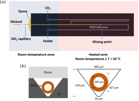
In this study, we have considered the design of a microfluidic reactor reproducing SAS experiment by contacting the solvent (ethanol) and the antisolvent (CO2) in a coflow geometry.

The microreactor was made in Silicon-Pyrex, which is a micro fabrication technology largely utilized for high pressure microfluidics (Couto et al., 2015; Marre et al., 2010), combining the mechanical properties of silicon and Pyrex with the good thermal conductivity of silicon and the visible transparency of Pyrex, thus providing an easy optical access.

(a)

(b)

Figure 1: Illustration of the developed microfluidic device used for the experimental mixing studies: (a). Top view of the general design and (b). cross-section views with additional details of dimensions.

The microchannel was first wet etched in silicon wafer following a photolithography step involving the UV exposure of a photoresist through a photomask on which the design was printed. Ultimately, the etched silicon wafer was anodically bonded to a top Pyrex cover. The microchannel cross-section is trapezoidal due to the

wet etching process. The general design of the microreactor is presented in Figure 1a. A main channel (top and bottom width of 400, 36 µm respectively and height of 234 µm), where the mixing occurs, is fed by a side channel aiming at preheating the CO2 flow. Then, a silica capillary (100 µm ID and 167 µm OD), used to introduce the solvent ethanol, is inserted inside the main channel and further epoxy glued to provide a full 3D injection as shown in the cross-section view of Figure 1b. This configuration allows working up to 150 bar in pressure. The temperature of the heated part of the chip is maintained thanks to a heating element controlled with an Eurotherm⃝ temperature controller.R

2.3

Experimental set-up and µPIV measurements

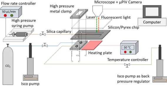
The microreactor is implemented in a general experimental set-up detailed in Figure 2. CO2 and ethanol are injected with an ISCO 100 DM pump equipped with a cooling jacket, and a Harvard PhD 2000 high pressure syringe pump, respectively. The pumps are connected to the microreactor and the silica capillary thanks to a house-made compression part and Valco/Vici commercial fittings, respectively, as seen in Figure 2. The overall pressure is controlled using another ISCO pump working downstream in constant pressure mode. A heating plate is placed on the silicon surface of the microchip to control the temperature. In order to acquire locally the fluid velocities during the injection and mixing process, the hydrodynamic inside the microreactor was characterized by an in-situ µPIV system. The µPIV set-up includes (i) a laser diode emitting at λ = 532 nm, which frequency is set to 4 Hz, with the pulse duration controlled at 15 µs with a time delay at 6 µs, (ii) a ZEISS Axiovert 200M microscope with a 20× magnification objective, (iii) a CCD camera of the Vieworks company displaying a resolution of 3296× 2472 pixels, with a frame rate of 10 fps. The PIV experimental data are processed by using the software Hiris, developed by R&D Vision company.

Figure 2: Microfluidic set-up developed for the µPIV analysis of the high pressure and controlled temperature mixing of CO2and ethanol inside a microchannel.

The general principle of this characterization consists in tracking the displacement of fluorescent particles, which follow the streamlines of the fluids. The particles, in suspension in the fluid, are excited by a laser inducing the fluorescence of the particles, which can be captured by a camera. In a typical measurement procedure, by comparing the particles’ positions between two pictures taken at a very short interval of time ∆t, one can

estimate the instantaneous velocity field and then the mean velocities of these particles, which are assumed to be the local velocity of the mixing fluids because the particle diameters are much smaller than the width of the microchannel, so they are supposed to follow the current streamlines in the fluid mixture.

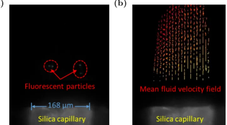
(a) (b)

Figure 3: Illustration of velocity field reconstruction by µPIV (a). A typical image of the acquisition mode of µPIV; (b). Mean velocity field of mixing fluids processed by Hiris software.

The tracer particles are preliminarily dried and diluted about 100 times in ethanol (0.01% of volume). The set-up is first pressurized gradually up to 100 bar from downstream with an ISCO pump filled with pure ethanol as a back pressure regulator. The liquefied CO2 is then injected by another ISCO pump in which the temperature is set originally at -5 ◦C and the pressure at 100 bar. Once the pressure and temperature are stabilized, the particle suspension in ethanol is injected inside the capillary thanks to a high pressure syringe pump. The two fluids encounter at the outlet of the capillary, forming a coflow mixing. While the laser arrives through the focused mixing zone, the particles in the microchannel are excited and return red fluorescent light at a wavelength of about 612 nm through a dichroic filter and captured by the camera. In a recorded acquisition of 1000 images (500 pairs), the tracer particle displacements can be observed in a black background to determine the average particle velocity field with a fixed interframe time ∆t of 100 µs. In the recorded images, the measured area is an adjustable rectangle of 0.5 mm× 0.3 mm (Figure 3). The images are integrated with a field depth of 10 µm. One pixel corresponds to 0.263 µm and the window size is chosen to be 64 pixels× 32 pixels, according to estimated fluid velocity. The reproducibility has been tested and the measurements are reproduced 3 times under fixed conditions (Figure 5 and Figure 6). During the experiment, no agglomeration of particles has been observed. However, some sedimentation is sometimes detected and some particles are trapped and attached to the wall. Nevertheless, according to the good reproducibility of the results, this effect could be neglected.

3

Numerical modeling

In the numerical modeling, the fluid velocity and ethanol concentration field are obtained by the resolution of the continuity equation, Navier-Stokes (NS) equation and the species transport equation. The effects of the presence of the fluorescent particles on the fluid properties are neglected so the mixture contains only CO2 and ethanol, which are supposed to be completely miscible in the investigated conditions according to their mixture phase diagram. Furthermore, the fluid flow is assumed to be isothermal.

3.1

Hydrodynamics

Since the mixture density relies only on the mixture composition and the conditions investigated, which always ensure the pressure above the critical point of the CO2-ethanol mixture, the equation of continuity (Equation 1) and the NS equation (Equation 2) are solved for a completely miscible and incompressible fluid mixture in one phase, as previously reported (Erriguible et al., 2013).

∇ · u = 0 (1)

ρ(∂u

∂t + u· ∇u) = −∇p + ∇ ·

(

µ(∇u + ∇Tu)) (2)

The ethanol mass fraction in the fluid mixture is calculated by the conservation equation of the species, according to the Fick’s law (Equation 3). The mass fraction of CO2can then be directly deduced.

∂ρxj

∂t +∇ · (ρxju− ρDj∇xj) = 0 (3)

3.2

Mixture thermophysical properties

In order to solve the equations mentioned in the model, it is necessary to have access or to calculate the thermophysical properties of the CO2-ethanol mixture, such as density, viscosity and diffusion coefficient.

The density of the fluid mixture is considered to be a function of its composition as well as the temperature and the pressure. It is calculated by the Peng Robinson equation of state (PREOS) (Equation 4) with Van der Waals mixing rules (Equation 5). The parameters a and b are solved first for pure components and then for the mixture. The interaction parameters kij and lij depend on the temperature (Maeta et al., 2015).

p = RT Vm− bm − am Vm(Vm+ bm) + bm(Vm− bm) (4) am= n ∑ i n ∑ j xixjaij bm= n ∑ i n ∑ j xixjbij (5) aij = (1− kij)(aiiajj)0.5 bij = (1− lij) bii+ bjj 2 a = 0.45724αR 2_T2 c Pc b = 0.0778RTc Pc α = ( 1 + (0.37464 + 1.5422ω− 0.26992ω2)(1− √ T Tc ) )2

The viscosities of the pure fluids are obtained from the NIST database for the considered experimental conditions and the mixture viscosity is calculated by a logarithmic mixing rule according to Equation 6:

ln µm= x_CO2ln µ_CO2+ xEtOHln µEtOH (6)

(Hayduk and Minhas, 1982; Fadli et al., 2010):

Dm= 1.33· 10−7· T1.47· V_EtOH−0.71· µ

10.2

V_{EtOH −}0.791

CO2 (7)

4

Results and discussion

4.1

Numerical procedure

The partial differential equations (1-3) are solved numerically to obtain the velocities and the species mass fractions for each time step, thanks to the CFD open source code “Notus” developed at the I2M/TREFLE Department. Meanwhile, the thermophysical properties are calculated at each time step according to local species composition. The approximation of the model described in Section 3 has been realized by the finite volume method on a fixed staggered grid. An implicit centered scheme is applied for all the terms in the Navier-Stokes equation while the transport equation is solved by a weighted essentially non-oscillatory (WENO) explicit scheme (Jiang and Shu, 1996). The gravity is neglected in the confined microchip because of a small value of the Bond number. The velocity–pressure coupling is solved by the solver BiCGSTAB II, preconditioned with a Jacobi method for the prediction step and the MCG approach for the correction step (Falgout and Yang et al., 2002).

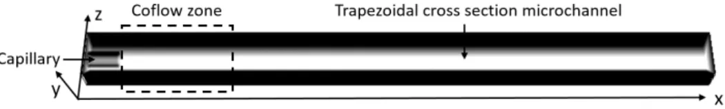
Due to the trapezoidal asymmetrical geometry, a three-dimensional simulation is required and the config-uration is exhibited in Figure 4. The whole shape of the simulated area is a cuboid of 0.6 cm× 0.023 cm × 0.04 cm. The circular injector has a length of 0.03 cm with an inner and an outer radius of 51 µm and 84

µm. Solid walls are penalized to shape the trapezoidal channel. The mean velocities for both CO2 and ethanol are provided at x = 0 based on the fluid flow rates and the fluid velocity is then developed by the simulation at the mixing point x = 0.03 cm. The ethanol mass fraction is defined to be 1 in the injector and 0 at the outside, leading to pure ethanol and pure CO2at x = 0 for the boundary conditions of species transport. The grid size is chosen to be 10 µm, according to a convergence study, which is comparable to the grid size of µPIV measurement (16.8 µm × 8.4 µm) so the total number of nodes is 552 000 (600 × 23 × 40). Given the high number of nodes required for describing the process with accuracy, the simulations are performed by a Message Passing Interface (MPI) parallel programming on 16 processors.

Figure 4: The 3D geometry of the microchannel in the CFD simulation.

4.2

Model validation

In order to validate the numerical model, the experimental and simulated data obtained for the fluid velocities were compared. The µPIV data were recorded on the mid cross-section of the channel corresponding

to the plane y = 0. First, the fluid velocities were measured in the microchannel far from the capillary tip, where the velocity profile is well developed and assumed to have a Poiseuille parabolic profile (Figure 5). Then, another area near the capillary tip was also investigated, in the mixing zone (Figure 6). The particles taken into account for the µPIV fluid velocity measurements can be actually at different height in the channel in a three-dimensional area with a fine thickness. However, as mentioned before, the thickness integrated with our equipment is 10 µm and one can consider that all the recorded particle movements are in a two-dimensional plane. For the case far from the injector, a comparison is shown in Figure 5b and both µPIV and numerical model provide similar results. The slight difference is probably due to the microfabrication procedure (wet etching step) as the microchannel can not be perfectly trapezoidal with smooth walls everywhere.

(a)

(b)

Figure 5: CFD validation for a fully developed flow (far from the injector): (a). 1D velocity comparison on the red dashed line far from the capillary outlet in the plane y = 0 (b). comparison at the mid-line for T = 22.5◦C, CO2 wt.%

= 93.6, with error bars according to replicated experiments (test No. 11 in Table 1).

Secondly, the fluid velocity at the capillary tip has been examined for different temperatures and fluid flow rates. Based on the experimental results, the velocity of the inner fluid (ethanol) drops first at the injector outlet. Actually the ethanol velocity in the capillary cannot be correctly measured by µPIV because the silica capillary reflects light and the particle movement inside it cannot be captured. However, the velocity of ethanol at the tip of the injector can be simply deduced from its flow rate. The fluid velocity increases then gradually in the x direction along with the outer fluid CO2. A one dimensional comparison is proposed in Figure 6 and data are retrieved from the mid-line of the 2D plane (red dashed line in Figure 6a).

In general, according to the two comparisons above, both experiments and simulations present similar hydrodynamic behaviors. The numerical model has been validated with simulated velocities in agreement with measured velocity profiles obtained by µPIV. We then used the CFD code to investigate the influence of various parameters on the mixing quality in the microfluidic chip.

(a)

(b) (c) (d)

Figure 6: CFD validation in the vicinity of the injector: (a). 1D velocity comparison at the capillary outlet on the red dashed line in the plane y = 0 (b). comparison at the mid-line with error bars according to replicated experiments for T = 22.5◦C, CO2wt.% = 93.6 (test No. 11) (c). T = 38◦C, CO2 wt.% = 83.1 (test No. 4) (d). T = 47.5◦C, CO2 wt.%

= 83.1 (test No. 5) in Table 1.

4.3

Fluid velocity and ethanol mass fraction field

A three-dimensional simulation case is presented in Figure 7a for the velocity component uxin the x direction

of the 2D plane y = 0. Similarly, the ethanol mass fraction field is shown in the 2D plane y = 0 (Figure 7b) and z = 0 (Figure 7c) for a Reynolds number of 1109, the temperature at 47.5◦C and the total mass fraction of CO2 at 93.7% (No.12 in Table 1). The black color symbolizes the silicon wall of the microchannel or the silica capillary tube. For the ethanol mass distribution, the red and blue colors represent the pure ethanol and the CO2, respectively. As expected, the simulation exhibits a mean field flow as no turbulent fluctuation is present.

(a)

(b)

(c)

Figure 7: y = 0, z = 0 views of the 3D simulation of the CO2-ethanol mixing in the microchip for T = 47.5◦C and

CO2 wt.% = 93.7 (No.12 in Table 1): (a) Velocity component ux field (y = 0 plane); (b) Ethanol mass fraction field (y

= 0 plane); (c) Ethanol mass fraction field (z = 0 plane).

Figure 7c shows the asymmetric ethanol mass fraction field in the plane z = 0. This result is related to the asymmetric trapezoidal shape of the channel and to the CO2 velocity, which is higher than the ethanol

at the injector outlet. The flow of CO2 first pushes the ethanol towards the bottom of the channel and the ethanol later goes up near the wall when the overall fluid velocity is higher in the center of channel, as indicated in Figure 8.

(a)

(b)

Figure 8: Ethanol mass fraction field and fluid velocity field variation in the asymmetrical 3D microchannel at steady state for T = 47.5 ◦C and CO2 wt.% = 93.7 (No.12 in Table 1): (a). Ethanol field evolution in the x direction; (b).

Velocity component ux evolution in the x direction.

4.4

Reynolds number, temperature and CO

/ethanol ratio effects on the mixing

quality

In this part, various simulation conditions have been performed to examine their effects on the mixing efficiency. All parameters are listed in Table 1, with average values calculated for the fluid velocity component

ux, the density ρ, the viscosity µ as well as the Reynolds number Re. These average values are described later.

(i) Mixing quality criteria

In order to investigate the effects of the process parameters on the mixing quality with simulated results of the validated numerical model, we have first defined a mixing index. The mixing quality is related to the homogeneity of the fluid mixture, which may be expressed classically by a relation known as the intensity of segregation or the mixing index (Equation 8) (Danckwerts, 1958):

Im=

∑

(xi− x)2

N· x · (1 − x) (8)

Table 1: Mixing conditions for the different simulation cases, along with the average fluid mixture properties and the characteristic time constant of mixing (∗initial velocity ratio of CO2to ethanol, based on the fluid flow rates).

No.

T

CO

Q

Q

u

u

u

ρ

µ

D

·10

Re

t

(

C)

(wt.%)

(µL

·min

)

(m

·s

)

(kg

·m

)

(µPa

·s) (m

·s

)

(ms)

1

20.0

82.8

25

100

0.0386

1.22

935

118

1.58

62

28.92

2

28.0

82.8

50

100

0.0802

1.37

896

96

1.86

152

18.65

3

22.5

82.9

50

200

0.0827

1.39

923

111

1.65

136

18.64

4

38.0

83.1

50

200

0.0903

1.85

843

72

2.34

208

14.28

5

47.5

83.1

50

200

0.0959

2.66

786

51

3.12

295

11.21

6

22.5

90.6

50

400

0.1559

2.77

896

90

1.65

308

7.74

7

38.0

90.8

50

400

0.1767

3.70

789

58

2.34

478

6.45

8

24.0

93.5

50

600

0.2326

4.20

864

80

1.70

499

4.74

9

38.0

93.6

50

600

0.2816

5.50

713

53

2.34

749

3.18

10

47.5

90.9

50

400

0.1972

5.37

706

40

3.12

697

4.46

11

22.5

93.6

50

600

0.2318

4.16

875

83

1.65

486

4.77

12

47.5

93.7

50

600

0.3143

8.06

644

36

3.12

1109

3.18

13

47.5

93.7

22

266

0.1391

8.07

644

36

3.12

491

3.88

14

47.5

90.7

23

180

0.0889

5.29

704

40

3.12

312

6.77

15

38.0

94.8

25

371

0.1690

6.86

732

51

2.34

478

3.66

16

38.0

97.7

10

351

0.1693

16.23

671

47

2.34

478

3.86

17

38.0

84.6

100

447

0.1998

2.07

836

69

2.34

478

11.59

the trapezoidal plane, N the total number of numerical grid elements in the cross-section. This index has a value ranging between 0 and 1, implying respectively a homogeneous mixture and a total segregation. Based on the simulation results, we have calculated this index for each trapezoidal cross-section as a function of the corresponding time:

t = ls ux

(9)

with lsthe distance to the injector outlet and uxthe mean fluid velocity component in the x direction far from

the injector for a fully developed and homogeneous flow, calculated assuming the mass flow rate conservation:

ux=

ρ_CO2Q_CO2+ ρ_EtOHQ_EtOH

ρA (10)

with ρ_CO2, ρ_EtOH the densities of pure CO2 and ethanol under the test conditions, Q_CO2, QEtOH the volumetric

flow rates in the microchip before mixing, ρ the density of complete mixture calculated by the global composition as well as A the trapezoidal area of the microchannel.

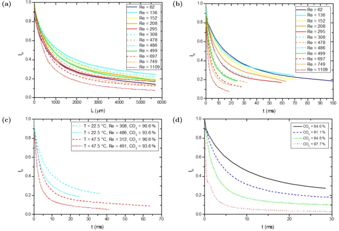
(ii) Influence of the total Reynolds number

We first have investigated the effect of the global Reynolds number on the mixing efficiency. Figure 9a and Figure 9b represent the evolution of the intensity of segregation calculated from the simulation for different average Reynolds numbers. Based on the simulation results, the Imvalues never reached 0 within the channel

whose the length is 6 mm, because a part of ethanol is pushed and trapped near the wall by CO2 with a high velocity due to the channel geometry, as shown in Figure 8. The average Reynolds number and the hydraulic

diameter of microchannel are defined as: Re = uxDhρ µ (11) where Dh= 4A P (12)

here µ the viscosity of complete mixture calculated by the global composition, Dh the hydraulic diameter,

estimated to be 200 µm for the microchannel and P the perimeter of the trapezoidal microchannel. It is not clear to determine the effect related to the Re number based on Figure 9a because of different mean velocities and the interest of introducing the time axis is to be able to compare with the characteristics mixing time published in the literature, which is discussed in the next part, so the length has been replaced by time for the axis, also resulting in the mixing index more comparable among different tests (Figure 9b). As expected, an improved mixing quality involves a higher global Reynolds number.

(a) (b)

(c) (d)

Figure 9: Mixing index / intensity of segregation Im derived from simulation results: (a). Im as a function of the

distance from the injector tip in the microchannel (b). Reynolds number effect on Im (c). Temperature effect on Im

with equivalent CO2/ethanol ratio and Reynolds number (d). CO2/ethanol ratio effect on Imwith fixed temperature at

38◦C and Reynolds number at 478.

(iii) Influence of the temperature

Then, the influences of the temperature have been also studied numerically and presented in Figure 9c. Near the critical temperature of the mixture CO2/ethanol, the temperature change has a strong effect on the mixture properties, such as density and viscosity and also on the molecular diffusion coefficient of ethanol in CO2. For a fixed CO2 flow rate, a higher temperature in the channel leads to a much lower CO2 density therefore a higher

velocity, according to the conservation of mass (Equation 13):

ρ0· Q0= ρT · Q (13)

where ρ0is the fluid density in the cooling pump, Q0 is the initial volumetric flow rate injected into the system by the pump, ρ_T is the fluid density in the microchannel at temperature T and Q is the real volumetric flow rate in the chip. Simulations have been performed to compare the evolution of the segregation intensity curve due to a temperature change, keeping an equivalent Reynolds number and fixed CO2/ethanol ratio in the mixture. As a matter of fact, it is impossible to examine the effect of each parameter independently, because some parameters are related. For example, when the temperature varies, in order to keep the same Reynolds number and the same CO2fraction in the system, the injected flow rates must be changed so the velocity ratio changes. Indeed, at laminar flow conditions, the mass transfer is related not only to the shear stress, but also to the diffusion in the perpendicular plane to the flow direction. As observed in Figure 9c, a higher temperature results in a quicker decrease of the mixing index value so the mixing quality is improved. This can be attributed to two main effects: first, the augmentation of the diffusion coefficient, and then, the change of the CO2 velocity due to a density decrease, leading to higher velocity ratio and consequently higher shear stress. For example, for the tests No.6 and No.14 in Table 1, the temperature increases from 22.5 ◦C to 47.5◦C, resulting in a rise of fluid velocity ratio (CO2 initial velocity over ethanol initial velocity) from 2.77 to 5.29.

(iv) Influence of the CO2/ethanol ratio

Eventually, we have investigated the effect of the CO2/ethanol ratio on the mixing efficiency. Figure 9d illustrates that a higher ratio promotes the mixing quality. When this parameter increases, it results in a tremendous difference of two fluids’ velocities. The strong shear stress at the capillary outlet due to an important CO2/ethanol ratio actually leads the CO2 flow towards the ethanol in the middle of the channel and improves mixing. The mean velocity of CO2 is 15 times higher than the ethanol velocity in the injector for the case of CO2 mass fraction of 97.7%, even creating recirculation vortices that improve significantly the mixing, shown in Figure 10 in which the velocity vectors are superimposed with the ethanol mass fraction field in the plane y = 0. The arrows in the figure represent only the velocity vector directions without magnitude. The same behavior has been captured in a numerical simulation for a two phase coflow in microfluidics (Zhang et al., 2018). However, for other cases of CO2lower than 97.7%, no recirculations were detected.

Figure 10: Recirculation detected in the mixing zone in the plane y = 0 for test case of which the CO2 mass fraction

is at 97.7%, with temperature at 38◦C and mean Reynolds number at 478.

We conclude that even if it is complicated to extract the influence of a single parameter over the mixing efficiency, we could identify some general trends based on the considered simulated cases. As expected, a higher

global Reynolds number results in a better mixing quality. An increase of the CO2/ethanol ratio enhances mass transfer in the mixture by increasing the shear stress generated by an important difference between the inner and the outer velocities at the injector outlet. This shear stress results in some cases in the creation of vortices near the tip of the nozzle, which largely contribute in decreasing the mixing time. According to the simulation results, a temperature increase improves the mixing because of both increased diffusion and shear stress. In general, a higher Reynolds number, an increased temperature and a strong CO2/ethanol ratio are recommended to accelerate fluid mixing.

4.5

Characteristic mixing time

Another important parameter for characterizing the mixing efficiency is the mixing time. A theoretical way to define the mixing time was proposed by Baldyga and Bourne (1986). It is defined as the time required to obtain a homogeneous mixture in a slab, considering both diffusion and advection mixing, also known as the stretching efficiency model (Equation 14). This equation has been largely applied to determine micromixer efficiency (Baldyga and Bourne, 1984; Falk and Commenge, 2010; Ghanem et al., 2014):

tm= 1 √ 2 √ ν ϵ ln 1.52· L · u D (14)

with ν the kinematic viscosity, ϵ the energy dissipation rate, L the characteristic length, u the fluid velocity and D the diffusion coefficient.

In this study, we have chosen to define the characteristic mixing time as the time constant of a first order system, which in here is the evolution of the segregation index as a function of the time. As illustrated in Figure 11, this time constant is defined as the intersection point of the time axis and the tangent of the origin of the mixing index curve.

Figure 11: Illustration of the mixing time constant determination for 2 different cases: the red one corresponds to the temperature of 47.5◦C and the CO2fraction of 93.7 wt.% (No.12); the blue one corresponds to the temperature of 22.5

◦_{C and the CO}

2fraction of 90.6 wt.% (No.6).

Similar method of tangent construction has been adopted to define a characteristic mixing length from supersaturation curve (Metzger, 2017). This mixing time definition reveals the decline rate of index value at the beginning of the mixing process, which is critical in SAS. Indeed, a mixing as quick as possible is desired

once the two fluids contact each other, in order to create high supersaturation and to promote nucleation. Since the theoretical mixing times in microchannels of different diameters published previously have been collected and correlated as a function of the energy dissipation rate ϵ (Falk and Commenge, 2010), the correlation was plotted and compared to our results in Figure 12. The energy dissipation rate for the laminar flow conditions employed in the present study has been determined by Equation 15:

ϵ = 26.12· ν · ux

2

Dh2

(15)

The coefficient 26.12 is recalculated, with details in appendix, according to the trapezoidal cross-section area of the microchannel (Bahrami et al., 2005).

The characteristic mixing times in this study (red points framed by two dotted lines illustrating a 50% relative error) are in agreement with the theoretical behavior shown as the blue line in Figure 12 (Falk and Commenge, 2010). Therefore, it seems that the determination of the mixing time in this study is an appropriate method to evaluate the mixing performance under laminar flow conditions for microfluidic coflow.

Figure 12: Comparison of characteristic time constant obtained in this study (red points) with the data published (blue line) in the literature (Falk and Commenge, 2010).

5

Conclusion

In this work, the CO2and ethanol mixture has been studied by both experimental and numerical approaches at microfluidic scale in laminar flow conditions. The mixing was studied under SAS process conditions, which means the two fluids are completely miscible in a single phase at 100 bar in a controlled temperature isother-mal environment. By applying a µPIV characterization, the fluid velocity was experimentally measured in a microchip considering a coflow configuration. A 3D CFD simulation has been validated by comparing the experimental and numerical results. Different average Reynolds numbers, the temperature between 20 and 50

◦_{C, as well as the ratio of CO}

2 to ethanol, have been investigated to capture their effects on mixing, which is characterized by the intensity of segregation or the mixing index Im. It has been discussed that these mixing

condition changes. We have obtained some tendencies of the conditions to achieve a fast mixing in the mi-crochannel. Finally, the mixing performance has been related to the characteristic mixing time constant, which is a simple criterion to examine the mixing efficiency in the micromixer. A first order system has been applied to estimate this mixing time constant according to the evolution of the mixing index curve as a function of time and this characteristic time has been well related to the energy dissipation rate ϵ of laminar flows. After comparing the mixing time constant of this study to the theoretical ones previously published, the results are reasonable and reliable. Therefore the method used in this paper is a robust way to study the laminar mixing of two different fluids under microfluidic SAS conditions.

Acknowledgement

This study was supported by the French National Research Agency (ANR-17-CE07-0029 - SUPERFON) and the University of Bordeaux (Ph.D. funding of Fan Zhang).

References

Aubin, J., Ferrando, M., Jiricny, V., 2010. Current methods for characterising mixing and flow in microchannels. Chemical Engineering Science 65: 2065–2093.

Bahrami, M., Yovanovich, M.M., Culham, J.R., 2005. Pressure drop of fully-developed, laminar flow in mi-crochannels of arbitrary cross-section. In 3rd International Conference on Mimi-crochannels and Minichannels. Baldyga, J., Bourne, J.R., 1984. A fluid mechanical approach to turbulent mixing and chemical reaction Part III: Computational and experimental results for the new Micromixing Model. Chemical Engineering Communications 28(4–6):259–281.

Baldyga, J., Bourne, J.R., 1986. Encyclopedia of Fluid Mechanics, Volume 1: Flow Phenomena and Measure-ment. Gulf Pub Co.

Baldyga, J., Czarnocki R., Shekunov B.Y., Smith K.B., 2010. Particle formation in supercritical fluids—Scale-up problem. chemical engineering research and design 88: 331–341

Boutin, O., 2012. Influence of introduction devices on crystallisation kinetic parameters in a supercritical antisolvent process, Journal of Crystal Growth 342: 13–20.

Campardelli, R., Reverchon, E., De Marco, I., 2017. Dependence of SAS particle morphologies on the ternary phase equilibria, The Journal of Supercritical Fluids 130: 273–281.

Chang, S., Lee, M., Lin, H., 2008. Role of phase behavior in micronization of lysozyme via a supercritical anti-solvent process, Chemical Engineering Journal 139: 416–425.

Couto, R., Chambon, S., Aymonier, C., Mignard, E., Pavageau, B., Erriguible, A., Marre, S., 2015. Microfluidic supercritical antisolvent continuous processing and direct spray coating of poly(3-hexylthiophene) nanoparticles for OFET devices. Chemical Communications, 51(6):1008–1011.

Danckwerts, P.V., 1958. The effect of incomplete mixing on homogeneous reactions. Chemical Engineering Science.

De Marco, I., Reverchon, E., 2011. Influence of pressure, temperature and concentration on the mechanisms of particle precipitation in supercritical antisolvent micronization, The Journal of Supercritical Fluids 58: 295– 302.

Erriguible, A., Fadli, T., Subra-Paternault, P., 2013. A complete 3d simulation of a crystallization process induced by supercritical CO2 to predict particle size. Computers & Chemical Engineering, 52:1–9.

Fadli, T., Erriguible, A., Laugier, S., Subra-Paternault, P., 2010. Simulation of heat and mass transfer of

CO2–solvent mixtures in miscible conditions: Isothermal and non-isothermal mixing. The Journal of Supercrit-ical Fluids, 52(2):193–202.

Falgout, R.D., Yang, U.M., 2002. hypre: A library of high performance preconditioners. In Lecture Notes in Computer Science, volume 2331, pages 632–641. Springer Berlin Heidelberg.

Falk, L., Commenge, J.-M., 2010. Performance comparison of micromixers. Chemical Engineering Science, 65(1):405–411.

Ghanem, A., Lemenand, T., Della Valle, D., Peerhossaini, H., 2014. Static mixers: Mechanisms, applications, and characterization methods – A review. Chemical Engineering Research and Design 92: 205-228.

Hayduk, W., Minhas,B.S., 1982. Correlations for prediction of molecular diffusivities in liquids. The Canadian Journal of Chemical Engineering, 60.

Jiang, G., Shu, C.W., 1996. Efficient Implementation of Weighted ENO Schemes. Journal of Computational Physics 126, 202-228. Article No. 0130.

Maeta, Y., Ota, M., Sato, Y., Smith, R., Inomata, H., 2015. Measurements of vapor–liquid equilibrium in both binary carbon dioxide–ethanol and ternary carbon dioxide–ethanol–water systems with a newly developed flow-type apparatus. Fluid Phase Equilibria, 405:96–100.

Marre, S., Adamo, A., Basak, S., Aymonier, C., Jensen, K.F., 2010. Design and packaging of microre-actors for high pressure and high temperature applications. Industrial Engineering Chemistry Research, 49(22):11310–11320.

Metzger, L., 2017. Process Simulation of Technical Precipitation Processes The Influence of Mixing. PhD thesis, Karlsruhe Institute of Technology.

Miguel, F., Martín, A., Mattea, F., Cocero, M.J., 2008. Precipitation of lutein and co-precipitation of lutein and poly-lactic acid with the supercritical anti-solvent process, Chemical Engineering and Processing 47: 1594–1602. Montes, A., Pereyra, C., Martinez de la Ossa, E.J., 2015. Screening design of experiment applied to the supercritical antisolvent precipitation of quercetin, The Journal of Supercritical Fluids 104: 10–18.

NIST (National Institute of Standards and Technology). <http://www.webbook.nist.gov/chemistry/>. Rossmann, M., Braeuer, A., Schluecker, E., 2014. Supercritical antisolvent micronization of PVP and ibuprofen sodium towards tailored solid dispersions, The Journal of Supercritical Fluids 89: 16–27.

Zhang, F., Erriguible, A., Gavoille, T., Timko, M.T., Marre, S., 2018. Inertia-driven jetting regimes in microflu-idic coflows. Physical Review Fluids, 3(9).

Appendix

Determination of the energy dissipation rate coefficient in a trapezoidal channel

For a laminar flow, the energy dissipation rate can be expressed based on Equation 16:

ϵ = Q∆p ρV = Q ρA · ∆p L (16)

with p the pressure, Q the flow rate, ρ the fluid density, V the container volume, A the cross-section surface and L the length of channel.

According to the Darcy-Weisbach equation (Equation 17) and the Darcy friction factor fD in a circular

tube Equation 18, one can easily obtain Equation 19: ∆p L = fD· ρ 2· u2 Dh (17) fD= 64 Re (18) ∆p L = 128µQ πDh4 (19)

with u the mean velocity, Dhthe hydraulic diameter, Re the Reynolds number, µ the fluid viscosity.

By combining Equation 16 and Equation 19, the energy dissipation rate ϵ is finally presented in Equation 20 for laminar flow in a circular tube:

ϵ =32ν(u)

2

Dh2

(20)

Above ϵ estimation is deducted only for fluid flow in a round cross-section conduit. Whereas, the coefficient 32 should be different for a different channel geometry. A similar correlation of Equation 18 is proposed for a trapezoidal shape channel, given Equation 21 (Bahrami et al., 2005):

fFRe√A=

8π2_(3ω2_{+ 1) + β(1− 3ω}2₎

9√ω(ω +√ω2− βω2_{+ 1)} (21)

in which fF is the Fanning friction factor and the Re√_A is the Reynolds number with the square root of

cross-sectional channel area as the characteristic length instead of the hydraulic diameter. The parameters ω and β are determined by the trapeze shape, shown in Figure 13.

ω = a + b

2h (22)

β = 4ab

(a + b)2 (23)

Figure 13: Schematic of trapeze cross-section geometry, extracted and modified from a published work (Bahrami et al., 2005).

calculated for a trapezoidal channel from Equation 24. By comparing Equation 18 and Equation 20 for the circular channel, the coefficient 26.12 is eventually derived for Equation 15.

fD=

52.24