Computer-aided analysis of critical technologies for hydrogen manufacture

by

L. B. Evans and J. E. Strong, Jr. MIT Energy Laboratory

COMPUTER-AIDED ANALYSIS

OF

CRITICAL TECHNOLOGIES FOR

HYDROGEN MANUFACTURE

by

Prof. Lawrence B. Evans John E. Strong, Jr.

Department of Chemical Engineering

M.I.T.

This informal working paper documents the results of a study to demonstrate and assess the applicability of flowsheet simulation or a

screening tool to aid in process research planning. Very crude models were used for three processes for hydrogen manufacture. Because of limitations in the model the process and economic results presented herein should be used only as an illustration of qualitative trends. We have not checked the data on which these results are based and make no claim for the exact numerical values.

The study demonstrated, however, that rigorous flowsheet simulation using ASPEN PLUS with preliminary process economics is an excellent tool for

evaluation processes at the research stage. If more time and data were

available, the models could be readily upgraded to give realistic quantitative comparisons.

ABSTRACT

The development of new chemical proce

hampered by exhaustive research into many var

several alternative production methods. Ther

need for a tool which can provide early infor guide the selection of the most promising rou identify the critical areas of research to ma

process most efficient. This study uses the

hydrogen manufacture, considered very importa

future of synfuels technology, to demonstrate

flowsheet simulation can fill this need.

sses is ofte iations in e is a real mation to he tes and ke the final example of In :1 nt for the how computer

Three different hydrogen production processes were

modeled with the ASPEN flowsheet simulation system. Steam

reforming and partial oxidation of methane were studied

separately and then compared. For each model the process

efficiency, defined in terms of product purity, yield, and

cost, was analyzed as a function of the operating

conditions. Trends in behavior were

methodologies for process optimizati

the processes, steam reforming was i cost effective process. Partial oxi resulting in lower initial capital i size plant, has higher operating cos need for a pure oxygen feed. This p with steam reforming only if a very

oxygen is available.

plotted and

on found. On comparing dentified as the more

dation, although

nvestment for the same ts associated with the rocess is competitive low cost source of

water.

differen

technologies.

simulated was electrolysis of

the method by which flowsheet

compare processes based on very

It was found that because of the cost of the large amount of electricity needed,

electrolysis produces hydrogen at several times the that of the steam reforming process. In addition, capital expenditure for a large scale electrolysis much higher than the same size steam reforming faci because of the high cost of the necessary electroly equipment. This suggests that electrolysis is not alternative for hydrogen manufacture on the scale n

for future synfuels processes.

cost as the plant is lity

sis

eeded

TABLE OF CONTENTS

ABSTRACT

TABLE OF CONTENTS

I.

PROCESS DESCRIPTIONS

Steam Reforming of Methane

Partial Oxidation of Methane .

Electrolysis of Water

8 . 13

. . .* .

*17

II.

ASPENPLUS FLOWSHEET SIMULATION

Steam Reforming of Methane

Partial Oxidation of Methane .

Electrolysis of Water

.

.

. . . . 21 .*

*

27

III. SIMULATION RESULTS

Steam Reforming of Methane

Partial Oxidation of Methane .

Electrolysis of Water

*

*.

IV.

CONCLUSIONS .

SOURCES CONSULTED .

APPENDIX: ASPEN Input Files

Listing 1: Steam Reforming of Methane .

Listing 2: Partial Oxidation of Methane

Listing 3: Electrolysis of Water

76 81 86 2 ·. . 3 . . . . . . . . . . . 4

4

INTRODUCTION

Although it is the third most abundant element by

atom, hydrogen does not appear naturally anywhere on earth

in its pure form. Generating hydrogen therefore requires

the chemical decomposition of a heavier material containing

hydrogen, followed by the separation of the gaseous

hydrogen from other side-products. (9) Because hydrogen

has been a very important feed stock in the chemical and petrochemical industries and because the production of it is typically quite expensive, a great deal of work and

money has gone into the development and optimization of the processes used to generate hydrogen. In the future

hydrogen should become an even more important raw material,

for although there is a world oil surplus at this time, the

certainty of long-term limited resources suggests the

eventual need for large quantities of hydrogen either as a fuel or in synthetic gas production. (4)

The oil crisis in the mid 1970's focused the

world's attention on the problem of limited resources and

the need to find alternative ways to insure reliable and inexpensive energy sources for the future. (9) One of the

critical areas identified was the need for efficient,

cheap, high-volume hydrogen production. As a result, an

explosion of research ensued on many fronts. People from

private industry, universities, and the United States

government all began large scale research projects. Some

looked at productio

hydrocarbons (e.g. improving the now f hydrocarbons (e.g. ways to make the si water, cost competi

inefficiency of ele cost of high-volume Finally, some explo

including the once

n methods involvi 1, 2, 4, and 11). avored process: s 1, 4, 7, 11, and

mplest method, di

tive despite the

ctricity generati

highly promising

Others looked at

inherent thermodynamic

on and the high capital ls (e.g. 3, 4, and 5).

production methods,

thermochemical cycles

involving complex multi-reaction systems in which water is

broken into its elements through the use of recycled reaction materials. (e.g. 4)

Among the many advancements forwarded by this

volume of work has been one fact inherent to hydrogen production: there is a vast number of production and

separation method combinations and no efficient way to

compare and choose among them. Some studies involved

detailed design and cost calculations for different

processes (4), but the inflexibility of this "brute-force" method becomes clear when one faces the task of repeating all of these calculations when a break-through is made in, for example, the physical reliability of very high

temperature reactors. Another comparative approach has

been the use of detailed computer models to predict

6

again an inherent inflexibility exists in that every time the process is modified in some way, a new computer program for the new process must be generated.

In the hydrogen industry, then, there is a clear need for a tool to aid in the study and selection of

alternative process pathways. An efficient method must be

developed by which processes which are vastly different in

concept and stage of development can be compared on an equal footing. With this tool, early development work

could be guided so as to eliminate improbable processes and

point out directions of greatest need for viable, low-cost

production methods. The desire for such a comparative tool is not exclusive to hydrogen production: there is a general need in the whole chemical industry for an efficient

methodology for process comparison.

This study focuses on one answer to this need:

computer flowsheet simulation. With flowsheet simulation,

the user is given a list of unit operations from which he may select. By taking those unit operations which are in the chemical process under study and connecting them

appropriately with material flow streams, a flowsheet

simulation is quickly developed. The user then has an

efficient means of studying the effects of any relevant

process inputs on any results of interest. The flexibility

of this method over "brute-force" calculations and

dedicated computer programs is clear when one considers the

ease with which the unit operations can be moved around,

inserted, or replaced in order to more fully explore

process alternatives.

The goal of this study is to demonstrate the power

of flowsheet simulation in studying, comparing, and

optimizing alternative processes. Various means of

hydrogen production, including steam reforming of methane,

partial oxidation of methane, and electrolysis of water,

have been selected for this demonstration because of the real and immediate need for this tool in this field as

described

ridge,

simulations,

methodology

production.

age

The flowsheet simulator ASPENPLUS,

.T. and now licensed by Aspen Technology, MA, was used for this work. This

1 of the unit operations necessary for hydrogen processes and has a comprehensive

with which capital and operating expenses

l culated.

d be noted that while every effort has been istic operating and cost numbers in these the emphasis

of flowsheet d cost conclu

It is hoped ity and appli

of this work is on the

simulation and not the specific sions found for hydrogen

that this demonstration will sh

cability of flowsheet simulatio

ow

n

to the study of alternative processes, and that engineers will use simulation in conjunction with actual data from

existing or experimental facilities to make intelligent

8

I. PROCESS DESCRIPTIONS

STEAM REFORMING OF METHANE

The first process to be simulated was the current

favored method for hydrogen production: steam reforming.

There are many variations on this process, including a variety of ways of treating the synthesis gas produced in the reformer and of separating the pure hydrogen from the side products. Figure 1 shows a typical configuration,

chosen because it is not overly complex and yet represents

the average process in use today.

The heart of this production method is the reformer furnace at the top of the flowsheet. Two feeds enter this

unit operation: steam and methane. Other hydrocarbons can

be used as the hydrogen source, but methane was selected because of its common use and because of its high hydrogen

to carbon ratio. After the feeds enter the reformer, they heat up and reaction takes place over a catalyst inside. The top of Figure 2 shows the reactions occuring in the

reformer. Methane and water react to form hydrogen and

carbon monoxide. The carbon monoxide can then react with

water to produce more hydrogen and carbon dioxide. The

overall reaction is highly endothermic, so the reformer furnace must supply heat to force the reactions to go

STEAM CO2 Q out Q out Q out Qin RECOVERED MEA WATER MEA

Process Flowsheet for Steam

Reforming

of

Methane

ODUCT . . . .

*

REFORMER REACTOR:

CH

H

0

3 H

CO + H

2

0

-*

C0

2

H

Temperature

Pressure

Steam: CH

* SHIFT REACTORS:

CO + H

0

-

CO

= 900 - 1250 K

= 10- 50 ATM

= 3.0 - 5.0

_H

Temperature = 600 - 750 K

(HIGH),

450

* METHANATOR:

CO

+ 4 H

4

CH

FIGURE 2:

Chemical Reactions for Reactors in Steam

Reforming Process

10

toward completion.

Also indicated on Figure 2 are broad ranges for the

reformer conditions. The temperature range is limited by

the effective range of the catalyst, and the pressure range is in part controlled by the need for high pressure

hydrogen at the end of the process (i.e. keep the pressure high throughout the process to avoid the costs of

compression at the end). The steam to methane ratio into

the reformer is generally about 4:1. The excess steam

helps drive both reactions toward the right, favoring

greater hydrogen production, and also helps prevent carbon

formation on the catalyst inside the reformer. (1)

The next step in the process, as shown in Figure 1, is a series of cooling and shift reaction steps. The

reformer exit gases are cooled and sent to a high

temperature shift reactor. Here some carbon monoxide is

converted to hydrogen over a catalyst via the water gas shift reaction. The center section of Figure 2 shows the

reaction involved. The exit from this reactor is cooled

again and sent to a low temperature shift reactor where

most of the remaining carbon monoxide is converted to

carbon dioxide and hydrogen. Also shown in Figure 2 are ranges in operating conditions for the two temperature

shift reactors. The temperatures are again limited by the

catalyst constraints.

This two step shift process is favored because of

the reaction equilibrium and cost of catalyst versus the

process temperature. Low temperatures favor near complete

conversion of carbon monoxide, but the catalysts active at

low temperature tend to be more expensive to use. (11) The

high temperature catalysts are cheaper, making it more cost

effective to shift some of the carbon monoxide over these catalysts and use a low temperature catalyst only as a

final, clean-up step.

The stream leaving the low temperature shift

reactor should contain a large fraction of hydrogen, some

carbon monoxide, some methane, and a small amount of carbon monoxide on a dry basis. The next step, as shown in Figure 1, is to remove the impurity carbon dioxide from the

product stream. Many methods are in use, but for this

simulation absorption with monoethanolamine (MEA) has been

used. Here the gaseous product stream is contacted on a multi-stage basis with the amine. Essentially all of the

carbon dioxide is removed in this way. The exit amine,

heavy with carbon dioxide, is sent on for recovery and

ultimate recycle. Usually, recovery is handled easily by

simply heating the MEA and driving off the carbon dioxide.

(4)

The product stream, now stripped of carbon dioxide,

contains hydrogen, methane, and carbon monoxide on a dry

basis. This stream is heated up so that the small amount

of carbon monoxide which was not shifted in the shift

reactors can be reacted in a methanator to produce the final product. The bottom of Figure 2 shows the reaction taking place in the catalytic methanator. A small amount

to give methane and water. As shown in Figure 1, all of the water in the product stream from the methanator is

removed, and the final product, consisting only of hydrogen

and methane, emerges.

PARTIAL OXIDATION OF METHANE

Another method for hydrogen production, which has

essentially been replaced by steam reforming, is partial oxidation. This process was selected as the second to be

simulated, for it is similar to steam reforming, providing

an easy basis of comparison, and it was hoped that the

simulation would demonstrate why steam reforming is

favored. Figure 3 shows the partial oxidation flowsheet used. The only major difference between this flowsheet and the steam reforming one shown in Figure 1 is the oxidizer at the top. Because both processes generate a synthesis

gas after their primary reactor, the exact same recovery

process was used downstream.

The feed to the oxidizer consists of methane, oxygen, and steam. Here too, other hydrocarbons can be used, including coal, as the hydrogen source. Methane was

selected simply to provide for easy comparison with the

steam reforming results. The top of Figure 4 shows the desired reactions taking place inside the oxidizer. The oxygen is used to oxidize the methane to produce hydrogen

STEAM CO₂ RECOVERED MEA Qout Qout Q out Qin WATER MLA

FIGURE

3: Process Flowsheet for Partial Oxidation of Methane

14

O') IMT

Ik row ! I Ai I

*

OXIDATION REACTOR:

CH

+(1/2)

02*

2

H

CO

H20

4

Co

+

H

Pressure

=

Steam: CH

=

02:

CH

* SHIFT REACTORS:

CO + H

0

-

CO

Terrperature

Pressure

1050 - 1300 K

0.5- 1.5

0.5-

1.5

+ H2

= 600 - 750 K

* METHANATOR:

CO

+

4H

2

4

CH

4 + 2 H

0

FIGURE 4: Chemical Reactions for Reactors in Partial

Oxidation Process

monoxide to produce more hydrogen and carbon dioxide.

Figure 4 also shows some ranges in operating

conditions. Depending on these process conditions, the

overall reaction may be either exothermic or endothermic.

This points up the real advantage to the partial oxidation

process: unlike steam reforming, little heat input is

required in this primary reactor, providing for savings on

capital to build the reactor and fuel costs while

operating. The disadvantage is the need for relatively

pure oxygen in large quantities. This usually requires

building an on-site oxygen plant as well, making the oxygen

an expensive feed stock. (11)

The steam to methane ratio for the oxidizer is far less than that in the reformer because water is not needed in the primary reaction. Generally a ratio of around 1.0

provides the necessary water to drive the second reaction

toward the right. The oxygen to methane ratio is also generally near 1.0. It must be high enough to allow the first reaction to take place but cannot be so high as to allow full oxidation to take place, burning off the desired

hydrogen.

The remainder of the partial oxidation flowsheet, as indicated in Figures 3 and 4, is the exact same as that

ELECTROLYSIS OF WATER

The final hydrogen generation process simulated

with this study was direct electrolysis of water. It is well known that electrical current, when applied to water

in an electrolysis cell, causes water to split into gaseous hydrogen and oxygen. This process is by far the simplest way to generate hydrogen and has the advantage of producing

almost 100% pure product with a minimum of separation

equipment. It suffers, however, from the high cost

associated with the large amount of electricity used and the large capital costs required for electrolysis cells

necessary for high volume production. Electrolysis was

selected for study so as to compare to the catalytic

methods of reforming and oxidation with the completely

different approach of electrolysis. It was hoped that the

simulation would demonstrate the advantages and

disadvantages between these processes, allowing for an

intelligent selection of the appropriate process for future

development.

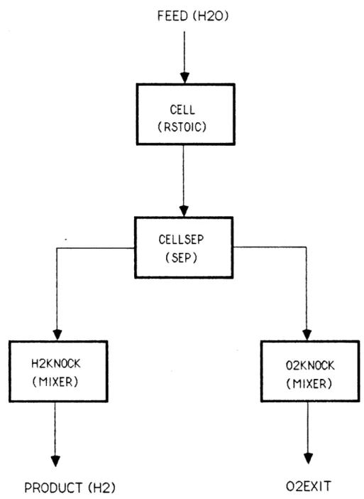
Figure 5 shows the simple flowsheet involved with

electrolysis. The water is fed to a cell where electricity is used to split it into its elements. The the product streams, oxygen and hydrogen, are then taken off. The pure oxygen created can be a bonus, however the high cost of

liquifaction needed to economically ship oxygen any great

distance negates this advantage unless the oxygen can be

18

WATER

ELECTRICITY

OXYGEN

HYDROGEN

Process Flowsheet

for

Electrolysis of Water

0

ELECTROLYSIS CELL:

+

electricity

-*

H

2

+ (1/2)

02

Reaction in Electolysis Process

H

0

Figure 6 shows what is happening chemically inside

the electrolysis cell. Again, the simple nature of the

process makes it attractive. The major complexity is

involved with the electrolyte which is used inside the

cell. Some systems use liquid electrolytes such as

solutions of potassium hydroxide. In order to improve cell

efficiency (theoretical power required divided by actual

power used), some work was been done to develop newer electrolytes such as solid polymers. (4) For this

simulation, it has been assumed that all of the feed water is converted to hydrogen and oxygen and that the overall cell efficiency is 85%.

II. ASPENPLUS FLOWSHEET SIMULATION

STEAM REFORMING OF METHANE

All of the simulations in this study were done with

the ASPENPLUS flowsheet simulation system. For each

process, the flowsheet was divided into its individual unit

operations. For each unit operation, ASPENPLUS has a

corresponding model or "block." Those blocks appearing in

a given flowsheet are selected and connected by material flow streams. The operating conditions for the unit

operations are entered and the feed streams are specified. The simulation can then be executed, and the desired

results accessed. In addition, ASPENPLUS has a

comprehensive costing section which allows the individual

process units to be costed, leading to a calculation of the total capital investment. The costing section also

calculates utility and raw material usage, labor, overhead,

and depreciation so that a total operating cost can be

reported.

Figure 7 shows the ASPEN block diagram for the steam reforming process. This shows all of the ASPEN

blocks used in this simulation and the types of models they represent. Listing 1 in the appendix shows the actual

FEED _~~~0 STEAM C02EXIT

...

T

4

'I

I

ii

(SEP)

]

ASPEN

block diagram for the Steam Reforming Process

REFORMER (RGI BBS) 22 COOL 1 (HEATER) HTSHI FT (RGIBBS) Fg -COOL2 (HEATER) - p

~~~~~~

,\,#

/V,

--v

r

.4

Figure 1 shows that the translation of

flowsheet to ASPEN block

step in the process with

The main reforme

reactor block "RGIBBS." free energy to find the the product stream. The

methane, water, hydrogen

dioxide - are entered in

conditions in the reform

approach to equilibrium

incomplete reaction. Fo

diagram consisted of matching each

the appropriate ASPEN model.

r reactor is modeled with the ASPEN

This is a model which uses Gibbs final equilibrium composition of

components which are present

-carbon monoxide, and -carbon

this block as are the operating er. Optionally, the temperature can be entered to simulate

r this simulation, the temperature approach to equilibrium for the methane reaction was set at

-15 C. (8)

All of the heaters and coolers are modeled with

"HEATER" blocks. These take as input the desired exit

temperature and pressure and calculate the necessary heat

duty based on the inlet stream conditions. This heat duty is then accessed by the costing section to determine heat exchanger and utility needs for the heating or cooling step.

Both the high temperature and low temperature shift

reactors are also modeled with "RGIBBS" blocks. Again the

species present and operating conditions are entered. For

both blocks a temperature approach to equilibrium of +10 C was used for the shift reaction. (8)

It was assumed that 100% of the carbon dioxide is removed by the monoethanolamine (MEA) in the scrubber. For

this reason,

block. This

dioxide.

"MEA-REC"

recovered

this step was modeled simply as a "SEP"

block takes the incoming flow of the gaseous d MEA and directs the individual species present :let streams with given separation fractions. For

ation 100% of the MEA exits with the stream going recovery unit as does 100% of the carbon

This stream goes to another "SEP" block,

which removes the carbon dioxide and returns the

MEA. The remaining gaseous materials in the

ll exit to the heater and on to the methanator. ie methanator is the only reactor which is not

th "RGIBBS." It was assumed that all remaining ioxide reacts to form water and methane (i.e. the goes idel to compl

"RSTOIC"

n).

ASPEN

conversion rate of that reaction. Here, a conversion rate of 1.0 was used.

The last unit in the flowsheet removes any water to produce a pure, dry product stream. This is a "SEP" block

in which all of the water is directed to the water exit stream and all of the hydrogen and methane is taken off as

product.

The costing section of the simulation

important variables from around the flowsheet

capital and operating costs. The heat duties size units such as the reformer furnace, the and the heating step, and the utility rates,

accesses the

to calculate are used to

cooling steps,

steam and fuel oil are calculated. Raw material usage, such as methane purchase cost, is also found. As will be discussed in the results section, one of the key uses for the costing section of the simulation was to take the production rate and operating cost and determine the production cost per million BTU of hydrogen for various

operating conditions.

PARTIAL OXIDATION OF METHANE

Because of the similarity between the processes,

the ASPEN simulation for partial oxidation was built

directly on that already developed for steam reforming.

Figure 8 shows the ASPEN block diagram for the partial oxidation process. Listing 2 in the Appendix is the

corresponding ASPEN input language. The only real

difference is in the first block - as mentioned above, the downstream processing of the synthesis gas is identical. For this process the oxidizer is modeled as a "RGIBBS"

reactor. Instead of just methane and steam, though, an

additional feed of pure oxygen is used. In the block, the presence of oxygen is added to the list of species found in the steam reformer reactor. It was assumed for this

simulation that the reactions taking place go to

equilibrium before exiting.

The remaining ASPEN blocks, input language, and

operating conditions are the same as those discussed above

26 CH4

--- No

pc

7v

1

,v'

(SEP)

ASPEN

_{block diagram for the Partial Oxidation Process}

OXIDIZER (RGIBBS) iiHEATER (HEATER) HTSHI FT (RGI BBS) COOL2 (HEATER) LTSHI FT (RGIBBS) C02EXIT

1

F

1

_

r

FIGURE 8:

.4

for steam reforming.

ELECTROLYSIS OF WATER

Electrolysis, being a fairly simple process, yields

a simple ASPEN block diagram, as seen in Figure 9. Listing 3 in the Appendix shows the ASPEN input language for this simulation. The feed, water, enters the electrolysis cell

which is modeled with an "RSTOIC" reactor. Here the

stoichiometry of water going to hydrogen and oxygen is specified. Since it has been assumed that all of the feed water is separated, the conversion fraction for this

reaction is set at 1.0.

Because only one exit stream is allowed for an "RSTOIC" block, the fact that hydrogen and oxygen are easily separated at the opp

the block "CELLSEP." This of the hydrogen and puts it

all of the oxygen and putti

Because occasionally liquid

exit gases, knock-out drums

that the product streams wi

The costing section

primarily of the capital ex cell and the cost of the el literature data, the instal

osite electrodes is modeled with

is a "SEP" block which takes all

in one exit stream while taking

ng it in the other exit stream. water can be entrained with the are put in the flowsheet so 11 be pure and dry.

of the simulation consists

penditure for the electrolysis

ectricity used. Based on some led capital cost was calculated on the basis of $300 per kw hydrogen heating value. (4)

28

FEED (H20)

PRODUCT (H2)

02EXIT

For the operating cost, no credit was given for the oxygen produced due to the fact that additional investment would be necessary to liquify the oxygen for shipping and it was assumed that there would be no use for oxygen on site.

30

III. SIMULATION RESULTS

STEAM REFORMING OF METHANE

The simulations developed for these hydrogen

production processes have been executed to show some

representative results and to demonstrate the potential of

flowsheet simulation. There are several ways to measure

the performance of a system. First, there is the purity of

the product stream. Generally, this stream will consist of

hydrogen and methane, and the closer it is to 100% hydrogen

the better. Second, there is the hydrogen production

rate. If the feed is held constant and the operating

conditions varied, not only will the purity change, but the production rate of hydrogen will also change. It might be possible, for example, to run the process in such a way as to get 95% pure hydrogen product while producing at a much lower rate than the potential. This would occur if a great

deal of carbon dioxide is produced, which is subsequently

removed. So both the purity and production rate are measures of how efficiently the feed is being converted

into hydrogen. Also of great importance in measuring the

performance of the system is the operating cost per unit of

hydrogen produced. This will tell if the plant is cost effective. All of these results will be looked at for the

simulations developed.

There are many parameters in the steam reforming

process which can be varied to change the performance of the system. Because the reformer reactor is the heart of

the system, however, only the operating conditions

associated with this unit have been studied. These include

the reformer temperature, reformer pressure, and feed steam

to methane ratio.

Figure 10 shows the fraction of hydrogen in the

process product stream (i.e. the purity - the remaining

fraction is all methane) as a function of the reformer temperature. Three curves are shown, each representing a different steam to methane feed ratio. It is clear that as

the temperature increases the reformer reactions are driven

toward the right, and the purity of the product stream increases. It is interesting to note that the purity

approaches 100% under all conditions at temperatures above 1200K. This suggests that operation above 1200K does not

gain much and research into higher temperature catalysts

and materials is not of great importance.

Figure 10 also shows that the higher the steam to methane ratio, the greater the final purity. Again this is because the excess steam tends to push the methane reaction

toward completion.

Figure 11 shows the product stream hydrogen purity

versus the reformer pressure. Here the purity drops as the

pressure increases, suggesting that higher pressure

32

900

FIGURE 10:

1000 1100 1200

REFORMER TEMPERATURE (K)

Fraction of hydrogen in the steam reforming product

stream versus reformer temperature for several steam

to methane

mole

ratios

with pressure = 20 ATM

R

A

0

T

F . R 1

A

0

0

T

REFORMER PRESSURE (ATM)

FIGURE

1:

Fraction of hydrogen in the steam reforming product

stream versus reformer pressure for several steam

to methane mole ratios

with

1100K

published literature data. (1) Again the different lines representing different steam to methane feed ratios show that excess steam helps to make the product stream more

highly concentrated in hydrogen.

Figure 12 shows the hydrogen production rate from a fixed methane feed versus the reformer temperature. The same trend as observed in Figure 10 is seen here. Higher

temperatures favor hydrogen production as do higher steam

flow rates.

Figure 13 shows a similar plot for hydrogen

production as a function of reformer pressure. It is clear that high pressure comes into direct conflict with high production rates from a given feed. This suggests that the process should be run at low pressure. Indeed, this is often done, however the desirability of high pressure

hydrogen at the end of the process becomes a problem.

Rather than investing in the compressor necessary to

produce this high pressure product, usually the pressure

throughout the process is kept high at the sacrifice of production rate. The suitability of one method or the

other depends on the required condition of the product

stream. For these simulations it has been assumed that pressurized hydrogen is desired (15 ATM or so) and that this pressure is achieved in the process and not with an

additional compressor.

Of primary concern in a process such as this is

determining the operating conditions which will produce

900

FIGURE 12:

1000 1100 1200 1300

REFORMER TEMPERATURE (K)

Daily hydrogen production rate from the steam reforming

process versus the reformer temperature for several

steam to methane mole ratios with pressure

=

20 ATM

H

2

0

A

T

m

s

c

f

a

36

10

FIGURE 13:

15 20 25 30

REFORMER PRESSURE (ATM)

Daily hydrogen production rate from the steam reforming

process versus the reformer pressure for several steam

to methane mole ratios

with temperature

1100K

2

0

m

d

a

y

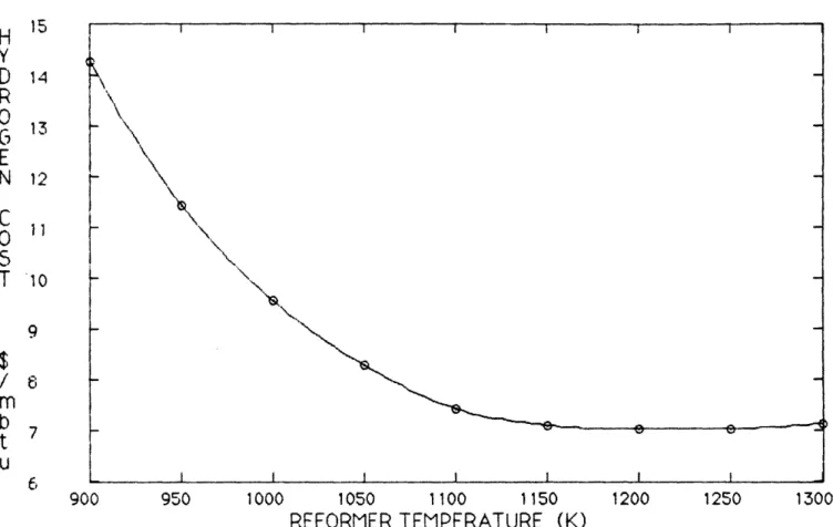
the cost of hydrogen production is plotted versus each of the operating variables. Figure 14 shows the steam

reforming operating cost per million BTU versus the

reformer temperature with the pressure set at 20 ATM and the steam to methane ratio at 4.0. The cost drops as

temperature increases but reaches an asymptotic limit at

about 1100K. With the pressure and steam rate set

accordingly, then, the optimum reformer temperature would

be about 1100K. In this way the temperature would be the

lowest possible while still producing the least expensive

hydrogen possible.

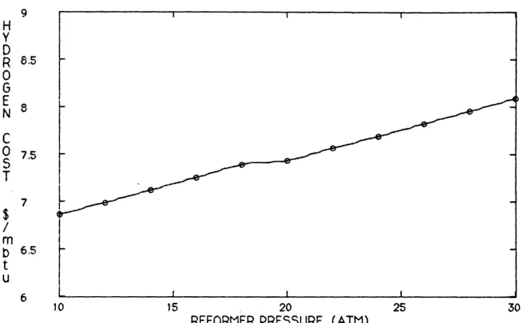
Figure 15 shows the hydrogen production cost as a function of the pressure with the temperature set at 1100K and the steam to methane ratio set at 4.0. Because of the

decrease in production associated with high pressures, the

operating cost rises with pressure. There is no way to look at this curve and select an optimum pressure. As

discussed above, the pressure must be selected from a

trade-off between cost and necessary exit pressure. For

the purposes of this simulation, a value of 20 ATM in the reformer has been assumed to be best - with pressure drops

in the process this yields about 14-15 ATM product.

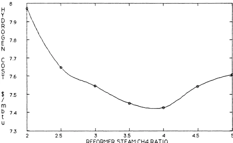
Figure 16 shows the hydrogen cost as a function of the steam to methane ratio with the temperature set at 1100K and pressure set at 20 ATM. At first, as the steam ratio increases, the cost drops. This is because, as

observed before, excess steam helps push the methane

reaction toward completion. However, above a ratio of

38

900 950 1000 1050 1100 1150 1200 1250 1300

REFORMER TEMPERATURE (K)

FIGURE 14: Cost of hydrogen produced by the steam reforming

process versus the reformer temperature with the

reformer pressure = 20 ATM, Steam:CH4 = 4.0

H lb Y D 14 R G 13 E N 12 C ₁₁

0

T

io

b

t

20

REFORMER PRESSURE

FIGURE 15:

_{Cost of hydrogen produced by the steam reforming}

process versus the reformer pressure with the

reformer

temperature

=

1 OOK,

Steam:CH4 = 4.0

9 8.5 8 7.5 7 6.5 H Y D R

0

0

S

T

t

u

u

(ATM)

2 2.5 3 3.5 4

REFORMER STEAM:CH4 RATIO

FIGURE 16:

Cost of hydrogen produced by the steam reforming

process versus the reformer steam:CH4 feed ratio

4.0 H Y D R

0

0

S

t

about 4.0 the cost begins to rise. This is probably due to the increased purchase cost of the steam and the heating requirements for bringing the incoming steam up to reaction

temperatures. The gain associated with excess steam above

a ratio of 4.0 is outweighed by the direct operating

costs. With the temperature and pressure set as indicated, then, the optimum steam to methane ratio for the reformer feed is 4.0.

It should be emphasized that the optimizations

discussed above are reasonably simplified. Each variable

was optimized individually with the other two fixed at some value. In a real process, all three would have to be

varied simultaneously in order to obtain the overall

process optimum.

With the reformer operating conditions set, it is informative to look at a "cross-section" of the process to

see what is happening. Figure 17 - obtained with data from

a run with the temperature at 1100K, the pressure at 20 ATM, and the steam to methane ratio at 4.0 - shows such a

cross-section. The dry mole percent of each species is

plotted versus the position in the process.

As indicated, the feed is pure methane. After the reformer, the methane percent has dropped to about 5% and

hydrogen is the dominant species at 75%. Carbon monoxide

and carbon dioxide are present in about equal

concentrations at 10%. In the shift reactors the carbon

monoxide is converted to hydrogen and carbon dioxide.

42

REFORM HT SHIFT LT SHIFT SCRUB PRODUCT

FIGURE 17:

_{Species profile of steam reforming process. The lines}

show the mole percent of each species in the streams

exiting the indicated unit operations

100

P

T

S

T

A

90

80

20

while the carbon dioxide and hydrogen curves rise. Methane

stays the same, for it is considered an inert in these

reactors.

After the scrubber, the carbon dioxide percent

drops to zero, for it has been removed. Because carbon dioxide was acting as a diluent, its removal causes the percentages of all of the other species to rise. The product stream shows the removal of all remaining carbon

monoxide by the methanator. The resulting product consists

of 95% hydrogen and 5% methane.

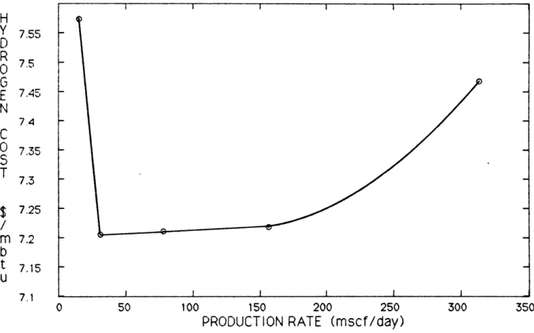
It is well known that different size plants will perform economically differently. As a final look at the steam reforming process, it is informative to look at the hydrogen cost as a function of the plant capacity. Figure 18 show such a plot. Because of the wide range of plant sizes covered (10 mscf/day to 300 mscf/day) three distinct areas emerge on this plot. At low capacity, a sharp

economy of scale is observed. There are minimum sizes for units such as reformer furnaces, and if the process is run below the limits of these units, it will be very expensive (high capital and operating cost spread over low production rates). Thus the cost drops as the size increases for low

production rates.

In the center of the figure, a relatively flat

region is observed. Here the process is being run at rates

easily handled by the equipment available. Increasing

production simple increases the capital and operating costs

50 100 150 200 250 300

PRODUCTION RATE

(mscf/day)

FIGURE 18:

Cost of hydrogen produced by the steam reforming

process versus the plant capacity with the reformer

temp = 1 1OOK, pressure = 20 ATM, steam:CH4 = 4.0

44

0

0

S

t

7.4

350

about the same.

At high production rates, however, larger and

larger pieces of equipment are necessary. As equipment

size increases, the costs tend to rise more quickly. Thus at high production rates the costs are increasing faster than the hydrogen produced, and the unit cost begins to rise.

As a basis of comparison with the other processes, the actual cost figures for a selected plant size have been summarized. Figure 19 shows this summary. As indicated, a medium size facility of 300 mscf/day was used. The

reformer operating conditions are indicated. The total

operating cost was found to be $7.43 per million BTU of

hydrogen which is in agreement with some representative

literature data. (9) As the pie chart indicates, the major pieces of the operating cost are raw materials (e.g.

methane and feed steam costs) and utilities (e.g. fuel oil and cooling water). The remainder of the cost is split

fairly evenly between labor, overhead, and capital

depreciation.

Also shown in Figure 19 is the capital investment required for a steam reforming plant this size. The total

bill would be about $300 million, split between process

unit purchase costs, setting labor, other directs such as

46

PLANT CAPACITY: 300 million scf per day

OPERATING

PARAMETERS:

Reformer Temperature = 1 OOK

Reformer Pressure

= 20 ATM

Steam:CH4

=4.0

OPERATING

COST = $ 7.43 per million btu hydrogen

Depreciation 4.5%

-

Overhead 5.3%

\ Labor 4.2%

CAPITAL COST SUMMARY:

Process Units

Other Directs

Setting Labor

Contingency

Working Capital

Start up Cost

TOTAL:

$

69,901,000

34,885,000

50,953,000

45,538,000

75,223,000

55,816,000

$ 332,316,000

FIGURE 19: Operating and capital cost breakdowns for a 300 mscf

per day hydrogen plant using steam reforming

PARTIAL OXIDATION OF METHANE

A similar analys has been made. In this steam reforming with par

many operating parameter

affect the system perfor

is wa ti ma ma

study concentrates only on

associated with the primar

operating parameters inclu

pressure, oxygen to methan

methane feed ratio. To li to methane ratio was set a this variable. The perfor as a function of the remai Figure 20 shows th function of the oxidizer t

represent different oxygen

of the partia y, it is possi al oxidation. in this proces nce. As with those operati

y reactor: the

1 oxidation process

oxidizer. These

r temperature, and steam to

slightly, the steam

ut to eliminate vs tem

three operating

emperature.

feed ratios

studied

nditions.

curves

rises. They all begin to reach an asymptotic limit at a temperature slightly over 1100K. This graph also indicates that the higher the oxygen to methane ratio, the higher the

purity of the product stream. This is because excess

oxygen drives the methane reaction to the right,

eliminating the methane from subsequent process streams.

Figure 21 shows the hydrogen product purity as

function of the oxidizer pressure. As with the reformer,

higher pressure tends to inhibit the reactions, decreasing

900

FIGURE 20:

1000 1100 1200

OXIDIZER TEMPERATURE (K)

Fraction of hydrogen in the partial oxidation product

stream versus the oxidizer temperature for several

oxygen

to

methane mole ratios

with pressure = 20 ATM

48 F R

A

0

P

0

R

A

0

0

OXIDIZER PRESSURE (ATM)

FIGURE

21: Fraction of hydrogen in the partal oxidation product

stream versus the oxidizer pressure for several

oxygen to methane mole ratios

with temperature = 1100K

30

the concentration of hydrogen in the product. This graph

suggests that higher oxygen to methane ratios not only

produce more pure product, but also tend to limit the

adverse effects of the higher pressures (compare the slope

of the 02:CH4=1.5 line with the 02:CH4=0.5 line).

Figure 22 shows the total hydrogen production rate

versus the oxidizer temperature. The production rate

increases then begins to level off at some point. This shows that similar to the reformer process there is no

great advantage to using temperatures above about 1200K for

partial oxidation. It is important to note that this

figure shows that low oxygen to methane feed ratios yield a higher production rate from a set methane feed. This is one of those cases in which the product purity conflicts with the production rate (compare Figures 20 and 22).

Excess oxygen forces more methane to react, increasing the

purity, but this same excess oxygen causes full oxidation

to take place, burning up some of the desired hydrogen. Figure 23 shows a similar plot for hydrogen

production rate versus oxidizer pressure. Increasing the

pressure drops the production rate. This highlights again

the conflict between production rate and desired product

pressure. Also shown is a confirmation of the fact that

higher oxygen to methane feed ratios give lower production

rates.

The effect of the operating conditions on the hydrogen cost will now be examined. Figure 24 shows the hydrogen cost per million BTU versus the oxygen to methane

1000 1100 1200 OXIDIZER TEMPERATURE (K)

FIGURE 22:

Daily hydrogen production rate from the partial oxidation

process versus the oxidizer temperature for several

oxygen to methane mole ratios

with pressure = 20 ATM

H

2

P

0

T

T

m

s

f

a

y

900

52

s15 20 25 30

OXIDIZER PRESSURE (ATM)

FIGURE 23:

Daily hydrogen production rate from the partial oxidation

process versus the oxidizer pressure for several oxygen

to methane mole ratios

with

1100K

H

2

0

T

m

f

y

.5 .6 .7 . .8 .9 1 1.1

OXIDIZER OXYGEN:CH4 RATIO

FIGURE 24:

Cost of hydrogen produced by the partial oxidation

process versus the oxidizer oxygen:CH4 feed ratio

w i th oxidi zer temp=

1 OOK,

pressure=20 ATM

0

0

t

feed ratio with the temperature set at 1100K and the pressure set at 20 ATM. Because of decreasing production rates, increasing the oxygen to methane ratio increases the hydrogen cost. This is also in part due to the increasing cost of the oxygen which must be supplied to the oxidizer. There is no way to select an optimum ratio from this

curve. There is a trade-off between cost and desired

product purity which can only be solved when the purity is

specified. In order to compare to the results from the steam reforming process, the desired purity was set at about 95%. Based on this, for the given temperature and pressure, the necessary oxygen to methane ratio is 1.0 (see Figure 20).

Figure 25 shows the hydrogen cost as a function of the oxidizer temperature with the oxygen to steam ratio set at 1.0 and the pressure set at 20 ATM. The cost drops as the temperature increases and then levels off. As with the

reformer process, the optimum temperature was taken as the lowest at which the cost is a minimum. From Figure 25 this optimum oxidizer temperature is seen to be about 1100K.

Figure 26 shows the hydrogen cost versus the

oxidizer pressure. The cost rises steadily as the pressure

increases. Again, an optimum cannot be determined without

a specification of the desired product pressure. For

comparison with the reformer process, an oxidizer pressure

of 20 ATM was selected.

Figure 27 shows a cross-section of the partial

950 1000 1050 1100 1150 1200 1250

OXIDIZER TEMPERATURE (K)

FIGURE 25:

Cost of hydrogen produced by the partial oxidation

process versus the oxidizer temperature with

oxidizer pressure=20 ATM, 02:CH4 = 1.0

22 20 18 16 14 12 10 8 H y D R

0

0

S

t

15 20 25 OXIDIZER PRESSURE (ATM)

FIGURE 26:

Cost of hydrogen produced by the partial oxidation

process versus the oxidizer pressure with the

oxidizer temp= 11 OOK, 02:CH4 = 1.0

56

0

0

t

u

FEED OXIDIZER HT SHIFT LT SHIFT SCRUB PRODUCT

FIGURE 27: Species profile of partial oxidation process. The lines

show the mole percent of each species in the streams

exiting the Indicated unit operations

100

P

S

T

40

A

reforming. The feed is pure methane, and after the

oxidizer the methane concentration drops to less than 5% on a dry mole basis. The carbon monoxide and carbon dioxide concentrations are about equal at 20%. Oxygen is not shown, for it was found to completely react in the

oxidizer. This leaves hydrogen at about 57%. Comparing

this to the steam reforming result shows that more carbon

oxides are formed in this process, yielding less hydrogen

from the primary reactor.

The two shift reactors show the carbon monoxide

being almost completely converted to carbon dioxide and

hydrogen. The scrubber removes all of the carbon dioxide,

and the methanator reacts the trace amounts of carbon

monoxide. The final product stream, as desired, is about

95% hydrogen and 5% methane.

Figure 28 shows the cost of the hydrogen as a

function of the plant capacity. Three curves are shown,

each representing a different oxygen purchase cost. It has

been suggested that the primary reason steam reforming is

favored over partial oxidation is because of the investment

necessary to produce the oxygen. (11) This investment can be translated into the oxygen purchase cost in order study

the effect of this cost on the viability of the process. As would be expected, this graph shows that cheaper oxygen

produces a cheaper hydrogen product. These curves will be

compared to the one from steam reforming later in this

section.

0 50 100 150 200 250 300 350

PRODUCTION RATE (mscf/day)

FIGURE 28: Cost of hydrogen produced by the partial oxidation process

versus the plant capacity for several oxygen purchase costs

with oxidizer

temp=1 lOOK, pres=20 ATM, 02:CH4 = 1.0

14 H Y D 1 3 R

0

0

S

T Io

m

b

8

t

u

02 Cost = 0.08 $/kg

02 Cost = 0.016 $/Kg

steam reforming are seen in Figure 28. At low production rate there is a sharp economy of scale. Yet as production increases, the costs rise faster than the capacity and the hydrogen cost slowly rises.

The operating and capital costs for a 300 mscf/day partial oxidation plant have been tabulated in Figure 29. The operating conditions are shown and the operating cost is seen to be $8.74 per million BTU hydrogen - about $1.30 more expensive than steam reforming. The operating cost breakdown is quite different for this process than that of steam reforming. The major cost is raw materials and

utilities take up less of the cost. This is because in partial oxidation the heat in the primary reactor is

supplied by the feed oxygen (a raw material) while in steam reforming the heat is supplied externally by burning fuel oil (a utility).

Figure 29 also shows the capital investment summary for a partial oxidation plant of this size. The total

investment would be about $186 million - $150 million lower

than the steam reforming process. The fact that the

capital is lower for partial oxidation is in large part due to the fact that the primary reactor is far less

complicated, requiring a lower purchase , setting, and

start-up cost.

PLANT

CAPACITY: 300 million scf per day

Oxidizer Temperature = 1100K

Oxidizer Pressure

= 20 ATM

Oxygen:CH4 = 1.0

Steam:CH4 = 1.0

OPERATING

COST = $ 8.74 per million btu hydrogen

~~-Depreciation 0.5%

~'-

Overhead 0.6%

Labor 0.5%

CAPITAL COST SUMMARY:

Process Units

Other Directs

Setting Labor

Contingency

Working Capital

Start up Cost

TOTAL:

$ 10,937,000

4,924,000

6,120,000

6,427,000

96,225,000

62,005,000

$ 186,638,000

FIGURE 29:

Operating and capital cost breakdowns for a 300 mscf

per day hydrogen plant using partial oxidation

-ELECTROLYSIS OF WATER

In the electrolysis simulation there are no real

operating conditions which can be varied. Although the

temperature and pressure can have some effect on the cell efficiency (4), for simplicity the cell efficiency in this simulation was assumed constant at 85%. The only operating parameter of interest, then, is the hydrogen production rate versus the feed flow rate. Figure 30 shows this

relationship. As would be expected, the production

increases linearly with the water feed rate. This graph

can be used to find the necessary water feed rate given a

desired production rate.

Figure 31 shows the cost performance of this

process. In the oxidation process the price of oxygen was the key cost factor. Here the cost of electricity is critical. The three curves shown in Figure 31 represent

different electricity purchase prices. In all cases the

cost of hydrogen increases with the plant capacity because

of the accelerating cost of high capacity electrolysis

cells. It is interesting to note that no economy of scale is observed at low production rate. This is because unlike

reformer or oxidizer reactors, electrolysis units do not

really have a minimum size. As expected, the lower the cost of electricity, the lower the product hydrogen cost.

Figure 32 shows the operating and capital cost

breakdowns for an electrolysis plant producing 300 mscf/day

5000

10000

15000

20000

25000

30000

FIGURE

30:

Daily hydrogen production rate from the electrolysis

system versus the water feed flow rate

H

2

0

0

s

c

f

d

y

210

60

30

100 150

PRODUCTION RATE

200

(mscf/day)

FIGURE 31;

Cost of hydrogen produced by electrolysis

versus the

plant capacity for several electricity purchase costs

64

0

0

S

T

b

t

u

30

Elec Cost = 0.06 $/kwhr

Elec Cost = 0.03 $/kwhr

Elec Cost

=

0.01 $/kwhr

c

~

~~~

I

I

~

~

1

~

,,I,

~~

50

PLANT CAPACITY: 300 million scf per day

Water Feed Rate = 30,000 kmol/hr

OPERATING

COST = $ 28.95 per million btu hydrogen

.

Raw Materials 0.2%

Labor

Overead

14.8%

/

\

18.7%S

Deprec

CAPITAL COST SUMMARY:

Process Units

Other Directs

Setting Labor

Contingency

Working Capital

Start up Cost

$ 1,179,678,000

447,250,000

369,746,000

583,823,000

289,498,000

259,989,000

$ 3,129,984,000

FIGURE

32: Operating and capital cost breakdowns for a 300 mscf