HAL Id: hal-01848554
https://hal.archives-ouvertes.fr/hal-01848554v2
Submitted on 20 Dec 2018
HAL is a multi-disciplinary open access
archive for the deposit and dissemination of
sci-entific research documents, whether they are
pub-lished or not. The documents may come from
teaching and research institutions in France or
abroad, or from public or private research centers.
L’archive ouverte pluridisciplinaire HAL, est
destinée au dépôt et à la diffusion de documents
scientifiques de niveau recherche, publiés ou non,
émanant des établissements d’enseignement et de
recherche français ou étrangers, des laboratoires
publics ou privés.
and One Reset
Alain Finkel, Jérôme Leroux, Grégoire Sutre
To cite this version:
Alain Finkel, Jérôme Leroux, Grégoire Sutre. Reachability for Two-Counter Machines with One
Test and One Reset. FSTTCS 2018 - 38th IARCS Annual Conference on Foundations of
Soft-ware Technology and Theoretical Computer Science, Dec 2018, Ahmedabad, India. pp.31:1-31:14,
�10.4230/LIPIcs.FSTTCS.2018.31�. �hal-01848554v2�
Test and One Reset
2Alain Finkel
3
LSV, ENS Paris-Saclay, CNRS, Université Paris-Saclay, France 4
Jérôme Leroux
6
LaBRI, Univ. Bordeaux, CNRS, Bordeaux-INP, Talence, France 7
Grégoire Sutre
9
LaBRI, Univ. Bordeaux, CNRS, Bordeaux-INP, Talence, France 10
Abstract
12
We prove that the reachability relation of two-counter machines with one zero-test and one reset 13
is Presburger-definable and effectively computable. Our proof is based on the introduction of two 14
classes of Presburger-definable relations effectively stable by transitive closure. This approach 15
generalizes and simplifies the existing different proofs and it solves an open problem introduced 16
by Finkel and Sutre in 2000. 17
2012 ACM Subject Classification Theory of computation → Logic → Logic and verification 18
Keywords and phrases Counter machine, Vector addition system, Reachability problem, Formal 19
verification, Presburger arithmetic, Infinite-state system 20
Digital Object Identifier 10.4230/LIPIcs.FSTTCS.2018.31 21
Funding This work was supported by the grant ANR-17-CE40-0028 of the French National 22
Research Agency ANR (project BRAVAS). 23
Acknowledgements The work reported was carried out in the framework of ReLaX, UMI2000 24
(ENS Paris-Saclay, CNRS, Univ. Bordeaux, CMI, IMSc). 25
1
Introduction
26
Context Vector addition systems with states (VASS) are equivalent to Petri nets and 27
to counter machines without the ability to test counters for zero. Although VASS have 28
been studied since the 1970’s, they remain fascinating since there are still some important 29
open problems like the complexity of reachability (known between ExpSpace and cubic-30
Ackermannian) or even an efficient (in practice) algorithm to solve reachability. In 1979, 31
Hopcroft and Pansiot [13] gave an algorithm that computes the Presburger-definable reach-32
ability set of a 2-dim VASS, hence VASS in dimension 2 are more easy to verify and they 33
enjoy interesting properties like reachability and equivalence of reachability sets, for instance, 34
are both decidable. Unfortunately, these results do not extend in dimension 3 or for 2-dim 35
VASS with zero-tests on the two counters: the reachability set (hence also the reachability 36
relation) is not Presburger-definable for 3-dim VASS [13] ; reachability, and all non-trivial 37
problems, are undecidable for 2-dim VASS extended with zero-tests on the two counters. 38
In 2004, Leroux and Sutre proved that the reachability relation of a 2-dim VASS is 39
also effectively definable [17] and this is not a consequence of the Presburger-40
© Alain Finkel, Jérôme Leroux and Grégoire Sutre; licensed under Creative Commons License CC-BY
Class Post∗ Pre∗ −→∗
T1Tr2' T1,2' T1,2R1,2Tr1,2 Not Recursive Not Recursive Not Recursive T1R2' T1R1,2Tr1 Eff. Presburger Eff. Presburger Eff. Presburger R1,2Tr1' R1,2Tr1,2 Eff. Presburger Eff. Presburger Eff. Presburger T1' T1R1Tr1 Eff. Presburger Eff. Presburger Eff. Presburger
2-dim VASS Eff. Presburger Eff. Presburger Eff. Presburger
Figure 1 Reachability sets (post∗ and pre∗) and reachability relation (−→) for extensions of∗ 2-dimensional VASS. We let ' denote the existence of mutual reductions between two classes of machines that preserve the effective Preburger-definability of the reachability sets and relation. The contributions of this paper are indicated in boldface.
definability of the reachability set. As a matter of fact, there exist counter machines (even 41
3-dim VASS) with a Presburger-definable reachability set but with a non Presburger-definable 42
reachability relation [13, 17]. But, for all recursive 2-dim extended VASS, the reachability 43
sets are Presburger-definable [11, 10]. More precisely, let us denote by TIRJTrK, with 44
I, J, K ⊆ {1, 2}, the class of 2-dim VASS extended with zero-tests on the I-counters, resets 45
on the J -counters and transfers from the K-counters. For instance, T{1}R{1,2}Tr∅, also 46
written T1R1,2 for short, is the class of 2-dim VASS extended with zero-tests on the first 47
counter, resets on both counters, and no transfer. The relations between classes from [11] are 48
recalled in Figure 1 and the class T1R2 has been shown to be the “maximal” class having 49
Presburger-definable post∗ and pre∗reachability sets [11]. However, it was unknown whether 50
the Presburger-definable reachability set post∗ can be effectively computed or not. In fact, 51
even the boundedness problem (is the reachability set post∗ finite?) was open for this class. 52
Contributions Our main contribution is a proof that the reachability relation of counter 53
machines in T1R2 is effectively Presburger-definable. Our proof relies on the effective 54
Presburger-definability of the reachability relation for 2-dim VASS [17]. The impact of our 55
result is threefold. 56
We solve the main open problem in [11] which was the question of the existence of 57
an algorithm that computes the Presburger-definable reachability set for two-counter 58
machines in T1R2. 59
In fact, we prove a stronger result, namely that the reachability relation of counter machines 60
in T1R2 is Presburger-definable and computable. This completes the decidability picture 61
of 2-dim extended VASS. 62
We provide a simple proof of the effective Presburger-definability of the reachability 63
relation in T1R2. As an immediate consequence, one may deduce all existing results [11, 64
10] for 2-dim extended VASS and our proof unifies all different existing proofs on 2-dim 65
extended VASS, including the proof in [6] that the boundedness problem is decidable for 66
the class R1,2 of 2-dim VASS extended with resets on both counters. 67
Related work VASS have been extended with resets, transfers and zero-tests. Extended 68
VASS with resets and transfers are well structured transition systems [9] hence termination 69
and coverability are decidable; but reachability and boundedness are undecidable (except 70
boundedness which is decidable for extended VASS with transfers) [5, 6]. The reachability and 71
place-boundedness problems are decidable for extended VASS with one zero-test [19, 3, 8, 4]. 72
Recently, Akshay et al. studied extended Petri nets with a hierarchy on places and with 73
resets, transfers and zero-tests [1]. As a counter is a particular case of a stack, it is natural 74
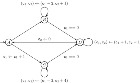
A B C D c1← c1+ 1 c1== 0 c1== 0 c2← 0 (c1, c2) ← (c1− 2, c2+ 1) (c1, c2) ← (c1− 2, c2+ 4) (c1, c2) ← (c1+ 1, c2− 1)
Figure 2 A 2-dimensional VASS extended with zero-tests on the first counter and resets on the
second counter (shortly called TRVASS).
to study counter machines with one stack. Termination and boundedness are decidable for 75
VASS with one stack [16] but surprisingly, the decidability status of the reachability problem 76
is open for VASS with one stack, both in arbitrary dimension and in dimension 1. We only 77
know that reachability and coverability for VASS with one stack are Tower-hard [14, 15]. 78
Outline We present in Section 2 an example of 2-dim extended VASS in T1R2. This 79
example motivates the study of two classes of binary relations on natural numbers, namely 80
diagonal relations in Section 3 and horizontal relations in Section 4. These two classes of 81
relations are combined in Section 5 into a new class of one counter automata with effectively 82
Presburger-definable reachability relations. These automata are used in Section 6 to compute 83
the reachability relations of 2-dim extended VASS in T1R2. 84
For the remainder of the paper, 2-dim extended VASS in T1R2are shortly called TRVASS. 85
2
Motivating Example
86
Figure 2 depicts an example of a TRVASS. There are four states A, B, C and D, and two 87
counters c1 and c2. Following the standard semantics of vector addition systems, these 88
counters range over natural numbers. The operations labeling the three loops and the edge 89
from A to C are classical addition instructions of vector addition systems. In dimension 2, 90
these addition instructions are always of the form (c1, c2) ← (c1+ a1, c2+ a2) where a1 and 91
a2are integer constants. For instance, the instruction (c1, c2) ← (c1− 2, c2+ 1) labeling the 92
loop on B means that c1 is decremented by 2 and at the same time c2 is incremented by 1. 93
As the counters must remain nonnegative, this instruction may be executed (i.e., the loop on 94
B may be taken) only if c1≥ 2. In addition to classical addition instructions, TRVASS may 95
test the first counter for zero, written c1== 0, and reset the second counter to zero, written 96
c2← 0. 97
The operational semantics of a TRVASS is given, as for vector addition systems, by an 98
infinite directed graph whose nodes are called configurations and whose edges are called steps. 99
Formal definitions will be given in Section 6. For the TRVASS of Figure 2, configurations 100
are triples q(x1, x2) where q ∈ {A, B, C, D} is a state and x1, x2 ∈ N are values of the 101
counters c1 and c2, respectively. It is understood that N denotes the set of natural numbers 102
{0, 1, 2, . . .}. There is a step from a configuration p(x1, x2) to a configuration q(y1, y2), 103
written p(x1, x2) → q(y1, y2), if there is an edge from p to q labeled by an operation (1) that 104
can be executed from the counter values (x1, x2) and (2) whose execution changes the counter 105
values from (x1, x2) to (y1, y2). Here, we have the steps B(5, 1) → B(3, 2), C(0, 2) → D(0, 2) 106
and D(7, 3) → A(7, 0). But there is no step from C(1, 2) and there is no step to A(7, 1). 107
The reachability relation of a TRVASS, written−→, is the reflexive-transitive closure of∗ the step relation →. The reachability relation is one of the main objects of interest for verification purposes. Coming back to our example of Figure 2, we have A(1, 0)−→ A(2, 0)∗ since we have the following contiguous sequence of steps:
A(1, 0) → C(2, 0) → C(0, 4) → D(0, 4) → D(1, 3) → D(2, 2) → A(2, 0)
By removing the steps → D(1, 3) → D(2, 2), we also get that A(1, 0)−→ A(0, 0). In fact, it∗ can be shown that A(1, 0)−→ A(y, 0) for every y ∈ N, thanks to the following pattern, where∗ k denotes an odd natural number and i ∈ {1, 2}:
A(k, 0) → C(k + 1, 0)−→ D(2k + 2, 0)∗ −→ D(k + i, k + 2 − i)∗ −→ A(k + i, 0)∗
One may wonder whether it also holds that A(x, 0) −→ A(y, 0) for every x, y ∈ N. A∗ 108
consequence of our main result (see Theorem 14) is that we can do even better: we can 109
compute the set of pairs (x, y) ∈ N×N such that A(x, 0)−→ A(y, 0), as a formula in Presburger∗ 110
arithmetic1. 111
IRemark. It is well-known that zero-tests are more expressive than resets. Indeed, a reset 112
c1← 0 can be simulated by a loop c1← c1− 1 followed by a zero-test c1== 0. A crucial 113
difference between resets and zero-tests is monotony. In a 2-dimensional VASS extended with 114
resets on both counters (shortly called RRVASS), larger counter values are always better, 115
in the sense that every behavior from a configuration q(x1, x2) can be reproduced from a 116
configuration q(x01, x02) with x10 ≥ x1 and x02 ≥ x2. This is not true anymore in presence 117
of zero-tests. This difference makes the analysis of TRVASS more complex than that of 118
RRVASS, as illustrated in the following example. J
119
IExample 1. Consider the RRVASS obtained from the TRVASS of Figure 2 by replacing the two zero-tests (from B to D and from C to D) with resets c1← 0. Suppose that we want to show that c1 is unbounded in state A from A(1, 0), i.e., A(1, 0)
∗
−→ A(y, 0) for infinitely many y ∈ N. A natural strategy is, starting from A(x, 0) with x ≥ 1, to reach D(0, y) with y as large as possible (without visiting A on the way), and then to reach A(y, 0) by taking the “transfer” loop on D as much as possible. By iterating this strategy, we get
A(1, 0)−→ D(0, 4)∗ −→ A(4, 0)∗ → D(0, 8)−∗ −→ A(8, 0)∗ −→ D(0, 16)∗ −→ A(16, 0) · · ·∗
This witnesses that c1 is unbounded in state A from A(1, 0). In comparison, this strategy does not work for the original TRVASS of Figure 2. Indeed, we get
A(1, 0)−→ D(0, 4)∗ −→ A(4, 0)∗ −→ D(0, 2)∗ −→ A(2, 0)∗ −→ D(0, 1)∗ −→ A(1, 0)∗
by following this strategy. This is because the only way to reach D from a configuration 120
A(x, 0) with x even is via B. J
121
The rest of the paper is devoted to the proof that the reachability relation of a TRVASS 122
is effectively Presburger-definable, i.e., there is an algorithm that, given a TRVASS and two 123
states p and q, computes a formula ϕ(x1, x2, y1, y2) in Presburger arithmetic whose models 124
are precisely the quadruples (x1, x2, y1, y2) of natural numbers such that p(x1, x2) ∗
−→ q(y1, y2). 125
It is already known that the reachability relation is effectively Presburger-definable in the 126
absence of zero-tests and resets [17]. Obviously, the counter c1 is zero after a zero-test 127
c1 == 0 and, similarly, the counter c2 is zero after a reset c2 ← 0. So we focus on the 128
reachability subrelations between configurations where at least one of the counters is zero, 129
for instance, {(x, 0, 0, y) | p(x, 0)−→ q(0, y)}. Such a subrelation can be seen as a (binary)∗ 130
relation on N. This motivates our study in Sections 3 and 4 of two classes of relations on N 131
that naturally stem from the operational semantics of TRVASS. 132
3
Diagonal Relations
133
We call a relation R ⊆ N × N diagonal when (x, y) ∈ R implies (x + c, y + c) ∈ R for every 134
c ∈ N. For instance, the identity relation on N, namely {(x, x) | x ∈ N}, is a diagonal relation. 135
The usual order ≤ on natural numbers is also a diagonal relation. It is readily seen that the 136
class of diagonal relations is closed under union, intersection, composition, and transitive 137
closure. In this section, we show that the transitive closure of a diagonal Presburger-definable 138
relation is effectively Presburger-definable. Our study of diagonal relations is motivated by 139
the following observation. 140
I Remark. The reachability subrelations {(x, y) | p(0, x) −→ q(0, y)}, where p and q are∗ 141
states, are diagonal in a TRVASS with no reset. Analogously, the reachability subrelations 142
{(x, y) | p(x, 0)−→ q(y, 0)} are diagonal in a TRVASS with no zero-test.∗ J 143
IExample 2. Let us consider the diagonal relation R ⊆ N × N defined by (x, y) ∈ R if,
144
and only if, the Presburger formula x ≤ y ∧ y ≤ 2x holds. It is routinely checked that 145
the transitive closure R+ of R satisfies (x, y) ∈ R+ if, and only if, the Presburger formula 146
(x = 0 ⇔ y = 0) ∧ x ≤ y holds. J
147
We fix, for the remainder of this section, a diagonal relation R ⊆ N × N. Consider the subsets IR and DRof N defined by
IR def
= {x | ∃y : (x, y) ∈ R ∧ x < y} DR def
= {y | ∃x : (x, y) ∈ R ∧ x > y} Since R is diagonal, the sets IR and DR are upward-closed, meaning that x ∈ IR implies 148
x0 ∈ IR for every x0 ≥ x (and similarly for DR). If x ∈ IR then (x, x + δ) ∈ R for some 149
positive integer δ > 0. Since R is diagonal, (x0, x0+ δ) ∈ R for every x0 ≥ x. So the pair 150
(x, x + δ) can be viewed as an “increasing loop” that applies to every x0 ≥ x. Similarly, if 151
y ∈ DRthen there is a “decreasing loop” (y + δ, y) ∈ R that applies to every y0≥ y. We are 152
mostly interested in increasing and decreasing loops that apply to every element of IR and 153
DR, respectively. This leads us to the following definitions: 154 α def= ( min{δ > 0 | ∀x ∈ IR: (x, x + δ) ∈ R} if IR6= ∅ 0 otherwise (1) 155 β def= ( min{δ > 0 | ∀y ∈ DR: (y + δ, y) ∈ R} if DR6= ∅ 0 otherwise (2) 156 157
Let us explain why the natural numbers α and β are well-defined. If IR 6= ∅ then there 158
exists δ > 0 such that (m, m + δ) ∈ R where m = min IR. It follows from diagonality 159
of R that (x, x + δ) ∈ R for every x ≥ m, hence, for every x ∈ IR. Therefore the set 160
{δ > 0 | ∀x ∈ IR : (x, x + δ) ∈ R} is non-empty, and so it has a minimum. A similar 161
argument shows that {δ > 0 | ∀y ∈ DR: (y + δ, y) ∈ R} is non-empty when DR6= ∅. 162
We are now almost ready to provide a characterization of the transitive closure of R+. 163
To do so, we introduce the relations IncR and DecR on N defined by 164 IncR(x, y) def = (x = y) ∨ (x ∈ IR ∧ ∃h ∈ N : y = x + hα) 165 DecR(x, y) def = (x = y) ∨ (y ∈ DR∧ ∃k ∈ N : x = y + kβ) 166 167
We let # denote relational composition (S # Rdef= {(x, z) | ∃y : x S y R z}). The powers of a 168
relation R are inductively defined by R1def= R and Rn+1def= R# Rn. 169
ILemma 3. It holds that R+= IncR# (R ∪ · · · ∪ R α+β+1)
# DecR. 170
Proof. We introduce the relation C = IncR# (R ∪ · · · ∪ R α+β+1)
# DecR, so as to reduce 171
clutter. To prove that C ⊆ R+, we show that Inc
R and DecRare both contained in R∗. Let 172
(x, y) ∈ IncR. If x = y then (x, y) ∈ R∗. Otherwise, x ∈ IR and there exists h ∈ N such that 173
y = x + hα. Moreover, h and α are positive as x 6= y. It follows from x ∈ IR and α > 0 that 174
(x, x + α) ∈ R. Since R is diagonal, we derive that (x, x + α), . . . , (x + (h − 1)α, x + hα) are all 175
in R. Hence, (x, y) ∈ R+. We have shown that Inc
R⊆ R∗. Now let (x, y) ∈ DecR. If x = y 176
then (x, y) ∈ R∗. Otherwise, y ∈ DRand there exists k ∈ N such that x = y + kβ. Moreover, 177
k and β are positive as x 6= y. It follows from y ∈ DR and β > 0 that (y + β, y) ∈ R. 178
Since R is diagonal, we derive that (y + kβ, y + (k − 1)β), . . . , (y + β, y) are all in R. Hence, 179
(x, y) ∈ R+. We have shown that DecR⊆ R∗. We derive from IncR ⊆ R∗ and DecR⊆ R∗ 180
that C ⊆ R+. 181
Let us now prove the converse inclusion R+⊆ C. We first observe that Inc
R = Inc∗R 182
and DecR= Dec∗R. These equalities easily follow from the definitions of IncR and DecR. As 183
a consequence, we get that 184 C = Inc∗R# (R ∪ · · · ∪ R α+β+1) # Dec ∗ R (3) 185
Let us prove by induction on n that Rn⊆ C for all n ≥ 1. The base cases n = 1, . . . , α + β + 1 are trivial. Assume that Rm⊆ C for all 1 ≤ m < n, where n ≥ α + β + 2, and let us show that this inclusion also holds for m = n. Let (x, y) ∈ Rn. There exists x0, . . . , xn such that x = x0R x1R · · · R xn= y. We start by showing the two following properties, as they will be crucial for the rest of the proof.
x 6∈ IR =⇒ x0≥ x1≥ · · · ≥ xn and y 6∈ DR =⇒ x0≤ x1≤ · · · ≤ xn We prove these properties by contraposition. If xi< xi+1 for some 0 ≤ i < n, then we may, 186
w.l.o.g., choose the first such i. This entails that x0 ≥ · · · ≥ xi. Moreover, xi ∈ IR since 187
xi < xi+1 and xiR xi+1. It follows that x = x0∈ IR as IR is upward-closed. Similarly, if 188
xi−1> xi for some 0 < i ≤ n, then we may, w.l.o.g., choose the last such i. This entails 189
that xi ≤ · · · ≤ xn. Moreover, xi ∈ DR since xi−1 > xi and xi−1R xi. It follows that 190
y = xn∈ DRas DR is upward-closed. 191
To prove that (x, y) ∈ C, we consider four cases, depending on the membership of x in 192
IR and on the membership of y in DR. 193
If x 6∈ IR and y 6∈ DR then x0= x1 = · · · = xn. This means in particular that x0R xn, 194
hence, x = x0C xn = y. 195
If x 6∈ IR and y ∈ DR then x0≥ x1≥ · · · ≥ xn. Note that β > 0 since DR is non-empty. 196
Since n ≥ β, there exists 0 ≤ i < j ≤ n such that xi≡ xj (mod β), hence, xi = xj+ kβ for 197
some k ∈ N. Recall that x = x0Rixiand xjRn−jxn = y. As R is diagonal, we derive that 198
xiRn−jy0 where y0 = y + kβ. We obtain that x Rn+i−jy0. It follows from the induction 199
hypothesis that x C y0. Moreover, we have (y0, y) ∈ DecR since y ∈ DR and y0 = y + kβ. 200
Hence, x (C# DecR) y and we derive from Equation 3 that x C y. 201
If x ∈ IR and y 6∈ DR then x0≤ x1≤ · · · ≤ xn. Note that α > 0 since IR is non-empty. 202
Since n ≥ α, there exists 0 ≤ i < j ≤ n such that xi ≡ xj (mod α), hence, xj = xi+ hα 203
for some h ∈ N. Recall that x = x0Rixi and xjRn−jxn= y. As R is diagonal, we derive 204
that x0Rix
j where x0 = x + hα. We obtain that x0Rn+i−jy. It follows from the induction 205
hypothesis that x0C y. Moreover, we have (x, x0) ∈ IncR since x ∈ IR and x0 = x + hα. 206
Hence, x (IncR# C ) y and we derive from Equation 3 that x C y. 207
If x ∈ IR and y ∈ DR then both α and β are positive. Since n ≥ α, there exists 208
0 ≤ i < j ≤ n such that xi≡ xj (mod α). If xi≤ xj then xj= xi+ hα for some h ∈ N and 209
we may proceed as in the case x ∈ IR∧ y 6∈ DR to show that x C y. Otherwise, xi= xj+ kα 210
for some k ∈ N. Recall that x = x0Rixi and xjRn−jxn = y. As R is diagonal, we 211
derive that x0Riz0Rn−jy0 where x0= x + kα(β − 1), z0= x
i+ kα(β − 1) = xj+ kαβ and 212
y0 = y + kαβ. We obtain that x0Rn+i−jy0. It follows from the induction hypothesis that 213
x0C y0. Moreover, we have (x, x0) ∈ IncR since x ∈ IR and x0= x + kα(β − 1), and we also 214
have (y0, y) ∈ DecR since y ∈ DR and y0 = y + kαβ. Hence, x (IncR# C # DecR) y and we 215
derive from Equation 3 that x C y. J
216
We derive the following theorem. 217
ITheorem 4. The transitive closure of a diagonal Presburger-definable relation is effectively
218
Presburger-definable. 219
Proof. Assume that ϕR(x, y) is a Presburger formula denoting a diagonal relation R. The 220
sets IR and DR are defined by the Presburger formulas ∃y : ϕR(x, y) ∧ x < y and ∃x : 221
ϕR(x, y) ∧ x > y, respectively. The natural numbers α and β defined in Equations 1 and 2 222
are obviously computable from ϕR. So the characterization given in Lemma 3 immediately 223
provides a computable Presburger formula denoting R+.
J
224
4
Horizontal Relations
225
A relation R ⊆ N × N is said to be horizontal if (x, y) ∈ R implies (x + c, y) ∈ R for every 226
c ∈ N. The class of horizontal relations is clearly stable by union, intersection, composition, 227
and transitive closure. In this section we prove that the transitive closure of a horizontal 228
Presburger-definable relation is effectively Presburger-definable. Our study of horizontal 229
relations is motivated by the following observation. 230
IRemark. The reachability subrelations {(x, y) | p(0, x)−→∗ c2←0
−−−→−→ q(y, 0)}, where p and q∗ 231
are states, are horizontal in a TRVASS. J
232
IExample 5. Let us consider the following horizontal relation R: R def= {(x, y) | 2y ≤ x ∨ (y ∈ 4N ∧ y ≤ 2x + 2)}
We prove that R+ is equal to C def= {(x, y) | x = 0 ⇒ y = 0} as follows. Since R ⊆ C and 233
C is transitive, we get R+⊆ C. Conversely, let (x, y) ∈ C. If x = 0 then y = 0 and from 234
(0, 0) ∈ R we derive (x, y) ∈ R+. So, we can assume that x ≥ 1. In that case (x, 4) ∈ R and 235
(4z, 4(z + 1)) ∈ R for every z > 0. It follows that (x, n) ∈ R+for every n ∈ 4 + 4N. Moreover, 236
there exists such an n satisfying 2y ≤ n. For such an n, we have (x, n) ∈ R+ and (n, y) ∈ R. 237
We deduce that (x, y) ∈ R+. It follows that R+= C.
J
238
The effective Presburger-definability of the transitive closure comes from the following 239
characterization. 240
ILemma 6. For every horizontal relation R we have:
241
R+ = {(x, y) | ∃z : (z, y) ∈ R ∧ ∀u : x ≤ u < z ⇒ ∃v : (u, v) ∈ R ∧ u < v} (4) 242
Proof. Assume first that (x, y) ∈ R+. There exists a sequence x0, . . . xk such that x = 243
x0R x1. . . R xk = y with k ≥ 1. Let z = xk−1 and let us prove that for every u ∈ 244
{x, . . . , z − 1} there exists v > u such that (u, v) ∈ R. If z ≤ x we are done. So we can 245
assume that z > x. Since x0≤ u, there exists a maximal j ∈ {1, . . . , k} such that xj−1≤ u. 246
Let v = xj and observe that (u, v) ∈ R. Since xk−1= z > u, it follows that j < k and by 247
maximality of j we deduce that xj> u. Therefore v > u. 248
Conversely, let us consider (x, y) ∈ N × N such that there exists z satisfying (z, y) ∈ R 249
and such that for every u ∈ {x, . . . , z − 1} there exists v > u such that (u, v) ∈ R. Notice 250
that there exists a sequence x0< · · · < xk with k ≥ 0 such that x = x0R x1. . . R xk≥ z. It 251
follows that (x, xk) ∈ R∗. Moreover, since (z, y) ∈ R, z ≤ xk, and R is horizontal we deduce 252
that (xk, y) ∈ R. It follows that (x, y) ∈ R+. J 253
The previous lemma shows that the transitive closure of a horizontal relation R denoted 254
by a Presburger formula ϕR is denoted by the Presburger formula obtained from (4) by 255
replacing (z, y) ∈ R and (u, v) ∈ R by ϕR(z, y) and ϕR(u, v) respectively. We have proved 256
the following theorem. 257
ITheorem 7. The transitive closure of a horizontal Presburger-definable relation is effectively
258
Presburger-definable. 259
5
Presburger Automata
260
We exhibit in this section a general class of one counter automata with effectively Presburger-261
definable reachability relations. These automata will be used in the next section to compute 262
the reachability relations of TRVASS. 263
A Presburger automaton is a pair P = (Q, ∆) where Q is a finite set of states, and ∆ 264
is a finite set of transitions (p, R, q) where p, q ∈ Q and R ⊆ N × N is a relation denoted 265
by a Presburger formula (which is left implicit). A configuration is a pair (q, x) ∈ Q × N, 266
also written as q(x) in the sequel. The one-step relation →P is the binary relation over 267
configurations defined by p(x) →P q(y) if there exists (p, R, q) ∈ ∆ such that (x, y) ∈ R. The 268
reachability relation −→∗ P is defined as the reflexive-transitive closure of →P. 269
IRemark. The reflexive-transitive closure R∗ of a Presburger-definable relation R ⊆ N × N 270
need not be Presburger-definable, in general. For instance, if R = {(x, y) ∈ N × N | y = 2x} 271
then R∗ is the relation {(x, y) ∈ N × N | ∃k ∈ N : y = 2kx}, which is not definable in 272
Presburger arithmetic. Worse, a simple reduction from the halting problem for Minsky 273
machines shows that membership of a pair (x, y) in R∗ is undecidable (where R is a 274
Presburger-definable relation given as input along with x and y). J 275
A consequence of the above remark is that the reachability problem for Presburger 276
automata is undecidable, even if we restrict ourselves to Presburger automata with a single 277
state and a single transition. This comes from the fact that transitions can use arbitrary 278
Presburger-definable relations. We will exhibit a subclass of Presburger automata with 279
effectively Presburger-definable reachability relations (hence, with a decidable reachability 280
problem) by limiting the expressive power of the transitions occurring on cycles. We say that 281
a transition (p, R, q) is diagonal if R is diagonal, horizontal if R is horizontal, and ordinary 282
if it is neither diagonal nor horizontal. Note that a relation on N may be both diagonal 283
and horizontal, for instance {(x, y) ∈ N × N | y ≤ 2x}. A cycle is non-empty sequence of 284
transitions (p1, R1, q1), . . . , (pn, Rn, qn) such that qn= p1 and qi= pi+1 for all 1 ≤ i < n. 285
ILemma 8. Let P be a Presburger automaton. If every cycle of P contains only diagonal
286
transitions then−→∗ P is effectively Presburger-definable. 287
Proof. We first observe that −→∗ P is effectively Presburger-definable when P = (Q, ∆) is 288
a Presburger automaton whose transitions are all diagonal. Indeed, we may view P as a 289
finite-state automaton over the finite alphabet {R | (p, R, q) ∈ ∆}. For every states p and q, 290
we may compute a regular expression denoting the language accepted by P with initial state p 291
and final state q. The obvious evaluation of this regular expression (concatenation · becomes 292
relational composition#, sum + becomes union ∪, and star ? becomes reflexive-transitive 293
closure ∗) yields the relation {(x, y) | p(x)−→∗ P q(y)}. This evaluation is computable because 294
Presburger-definable diagonal relations are effectively closed under union, composition and 295
reflexive-transitive closure (as an immediate consequence of Theorem 4). We have shown 296
that−→∗ P is effectively Presburger-definable when all transitions of P are diagonal. 297
We now prove the lemma. Let P = (Q, ∆) be a Presburger automaton such that every cycle of P contains only diagonal transitions. Let N be the Presburger automaton obtained from P by keeping only diagonal transitions. Consider two configurations p(x) and q(y). It is readily seen that p(x)−→∗ P q(y) if, and only if, there exists 1 ≤ k ≤ |Q|, s1, . . . , sk∈ Q and x1, y1, . . . , xk, yk ∈ N such that p(x) = s1(x1), sk(yk) = q(y) and
s1(x1) ∗ −→P s1(y1) →P s2(x2) ∗ −→P s2(y2) · · · sk−1(yk−1) →P sk(xk) ∗ − →P sk(yk) Observe that for every state s ∈ Q and for every x, y ∈ N, s(x)−→∗ P s(y) if, and only if, 298
s(x)−→∗ N s(y). Moreover, −→∗ N is effectively Presburger-definable since all transitions of N 299
are diagonal. We derive from the above characterization of−→∗ P that ∗
−→P is also effectively 300
Presburger-definable. J
301
We say that a Presburger automaton P is shallow if every cycle that contains an ordinary 302
transition also contains a horizontal transition. Shallowness of Presburger automata is 303
decidable. This follows from two easy observations. Firstly, diagonality and horizontality of 304
Presburger-definable relations on N are decidable, since these properties can be expressed in 305
Presburger arithmetic. Secondly, a Presburger automaton is shallow if, and only if, every 306
simple cycle containing an ordinary transition also contains a horizontal transition. We now 307
show the main result of this section. 308
ITheorem 9. The reachability relation of a shallow Presburger automaton is effectively
309
Presburger-definable. 310
Proof. By induction on the number of horizontal transitions. The base case follows from Lemma 8. Indeed, if P is a shallow Presburger automaton with no horizontal transition then every cycle of P contains only diagonal transitions. Assume that the theorem holds for every
shallow Presburger automaton with n horizontal transitions, where n ∈ N. Let P = (Q, ∆) be a Presburger automaton with n + 1 horizontal transitions. Pick a horizontal transition (p, R, q) ∈ ∆ and let N be the Presburger automaton obtained from P by removing the transition (p, R, q). Note that, by construction, N is shallow since P is shallow. Let S denote the reachability relation from q to p in N , namely the relation S = {(y, x) | q(y)−→∗ N p(x)}. It is readily seen that, for every configurations s(x) and t(y) of P, s(x)−→∗ P t(y) if, and only if, s(x)−→∗ N t(y) or there exists x0, y0∈ N such that
s(x)−→∗N p(x0) ∧ (x0, y0) ∈ ((R# S ) ∗
# R) ∧ q(y 0) ∗
−→N t(y)
By induction hypothesis, the relation−→∗ N is effectively Presburger-definable, and so is R# S . 311
Moreover, R# S is horizontal since R is horizontal. It follows from Theorem 7 that (R # S )∗ 312
is effectively Presburger-definable. We derive from the above characterization of−→∗ P that 313
∗ −
→P is also effectively Presburger-definable. J
314
IRemark. The notions of diagonal relations, horizontal relations and Presburger automata 315
are extended to larger dimensions in the obvious way. A relation R ⊆ Nd× Nd is diagonal 316
(resp. horizontal) if (x, y) ∈ R implies (x + c, y + c) ∈ R (resp. (x + c, y) ∈ R) for every 317
c ∈ Nd. But Theorem 9 does not extend to larger dimensions, even if we restrict ourselves 318
to Presburger automata with a single state and a single transition. In fact, the reflexive-319
transitive closure of a Presburger-definable relation that is diagonal (resp. horizontal) need 320
not be Presburger-definable. Consider the relation R ⊆ N2× N2defined by (x
1, x2) R (y1, y2) 321
if, and only if, the Presburger formula y1 ≤ 2x1∧ y2 < x2 holds. The relation R is both 322
diagonal and horizontal. It is routinely checked that the reflexive-transitive closure R∗ is the 323
set of pairs ((x1, x2), (y1, y2)) ∈ N2× N2such that y1≤ 2x2−y2x1 and y2≤ x2, which is not 324
definable in Presburger arithmetic. J
325
6
Reachability Relations of TRVASS
326
A TRVASS is a 2-dimensional vector addition system with states (2-dim VASS) such that the first counter can be tested for zero and the second one can be reset to zero. Formally, a TRVASS is a triple V = (Q, Σ, ∆) where Q is a finite set of states, Σ ⊆ Z2∪ {T, R} is a finite set of actions, and ∆ ⊆ Q × Σ × Q is a finite set of transitions. A configuration of V is a triple (q, x1, x2) ∈ Q × N × N written as q(x1, x2) in the sequel. The operational semantics of V is given by the binary relations−→a V over configurations, with a ∈ Σ, defined by p(x1, x2) a −→Vq(y1, y2) if (p, a, q) ∈ ∆ and (y1, y2) = (x1+ a1, x2+ a2) if a = (a1, a2) ∈ Z2 (y1, y2) = (0, x2) ∧ x1= 0 if a = T (y1, y2) = (x1, 0) if a = R Given a word w = a1. . . ak of actions aj ∈ Σ, we denote by
w
−→V the binary relation over 327
configurations defined as the relational composition a1
−→V # · · · # ak −→V. The relation ε − →V 328
denotes the identity relation on configurations. Given a subset W ⊆ Σ∗, we let −→W V denote 329 the unionS w∈W w −→V. The relation Σ∗ −−→V, also written ∗
−→V, is called the reachability relation 330
of V. Observe that−→∗ Vis the reflexive-transitive closure of the step relation →V def =S a∈Σ a −→V. 331
The remainder of this section is devoted to the proof that TRVASS have effectively 332
Presburger-definable reachability relations. Let us fix a TRVASS V = (Q, Σ, ∆). We let A 333
denote the set Σ ∩ Z2 of addition vectors. 334
The reachability relation of V can be expressed in terms of the reachability relation of a Presburger automaton by observing that configurations reachable just after a zero-test T or a reset R are restricted to q(0, n) or q(n, 0), respectively, where q ∈ Q and n ∈ N. Those configurations are parametrized by introducing the set S = {qT, qR| q ∈ Q} obtained as two disjoint copies of Q. Elements in {qT | q ∈ Q} are called test states, and those in {qR
| q ∈ Q} are called reset states. Given s ∈ S and n ∈ N, we introduce the configuration Js, nK in Q × N 2 defined as follows: Js, nK def = ( q(0, n) if s = qT q(n, 0) if s = qR
We also introduce, for each pair (s, t) ∈ S × S, the binary relation Rs,t defined by Rs,t
def
= {(m, n) ∈ N × N |Js, mK A∗X
−−−→VJt, nK}
where X = T if t is a test state and X = R if t is a reset state. It is known that the 335
reachability relation of a 2-dim VASS is effectively Presburger-definable [17, 2]. This entails 336
that the relation A ∗
−−→V is effectively Presburger-definable, and it follows that the relations 337
Rs,t are also effectively Presburger-definable. We introduce the Presburger automaton P 338
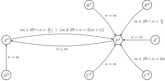
with set of states S and set of transitions {(s, Rs,t, t) | (s, t) ∈ S × S}. Note that P is 339 computable from V. 340 AR DT AT BT CT BR CR DR n ≤ m (m ∈ 2N ∧ n = m 2) ∨ (m 6∈ 2N ∧ n = 2(m + 1)) n = m m ∈ 2N ∧ n = m2 n = m m ∈ 2N ∧ n = 2m n = m n = m
Figure 3 The Presburger automaton P associated to the TRVASS of Figure 2.
IExample 10. Let us come back to the TRVASS of Figure 2. The relations Rs,tare all 341
empty except for RDT,AR, RDR,AR and Rs,DT with s ∈ {AT, AR, BT, BR, CT, CR}. The
342
corresponding automaton P is depicted in Figure 3. Each transition (s, Rs,t, t) is depicted 343
by an edge from s to t labeled by a Presburger formula ϕs,t(m, n) denoting the relation Rs,t. 344
The empty relations (which are both diagonal and horizontal) are not depicted. Notice that 345
the transition from ARto DT is ordinary and the one from DT to ARis horizontal. It follows 346
that P is shallow. We observe that the horizontal relation R defined as the composition 347
RDT,AR# RAR,DT is the one introduced in Example 5. J
348
We first show that the Presburger automaton P is shallow. By Theorem 9, this will entail 349
that its reachability relation−→∗ P is effectively Presburger-definable. 350
ILemma 11. The Presburger automaton P is shallow.
351
Proof. It is readily seen that P satisfies the following properties: 352
Transitions from reset states to reset states are diagonal, 353
Transitions from test states to reset states are horizontal, 354
Transitions from test states to test states are diagonal. 355
It follows that an ordinary transition of P is a transition from a reset state to a test state. If 356
a cycle contains such a transition then it must contain a transition from a test state to a 357
reset state as well. Since such a transition is horizontal, we obtain that P is shallow. J 358
The two following lemmas show how to decompose the reachability relation of V in terms 359
of the reachability relation of P. 360
ILemma 12. For every s, t ∈ S and m, n ∈ N, if s(m)−→∗ P t(n) then Js, mK ∗
−→VJt, nK. 361
Proof. It is easily seen that s(m) →P t(n) impliesJs, mK ∗
−→VJt, nK, for every s, t ∈ S and 362
m, n ∈ N. We derive, by an immediate induction on k ≥ 1, that s(m) (→P)k t(n) implies 363
Js, mK ∗ −
→VJt, nK, for every s, t ∈ S and m, n ∈ N. The lemma follows. J 364
I Lemma 13. Consider two configurations p(x1, x2) and q(y1, y2) of V. It holds that
p(x1, x2) Σ∗\A∗
−−−−→Vq(y1, y2) if, and only if, there exist s, t ∈ S and m, n ∈ N such that:
p(x1, x2) A∗{T,R} −−−−−−→VJs, mK ∧ s(m) ∗ −→P t(n) ∧ Jt, nK A∗ −−→Vq(y1, y2)
Proof. Lemma 12 shows the “if” direction of the equivalence. For the other direction, let w ∈ Σ∗\A∗ such that p(x
1, x2) w
−→V q(y1, y2). By splitting w after each occurrence of an action in {T, R}, we deduce that w = w0X1. . . wk−1Xkwkwhere k ≥ 1, and w0, . . . , wk∈ A∗. Let us introduce the configurations c1, . . . , ck satisfying the following relations:
p(x1, x2) w0X1 −−−→V c1· · · wk−1Xk −−−−−→V ck wk −−→V q(y1, y2) Notice that cj =Jq Xj
j , njK for some qj ∈ Q and some nj ∈ N. By definition of P, we get 365
qXj−1
j−1 (nj−1) →P q Xj
j (nj) for every j ∈ {1, . . . , k}. We have proved the lemma. J 366
We deduce our main result. 367
ITheorem 14. The reachability relation of a TRVASS is effectively Presburger-definable.
368
Proof. Lemma 13 shows that p(x1, x2) ∗
−→Vq(y1, y2) if, and only if, p(x1, x2) A∗
−−→Vq(y1, y2) or there exists s, t ∈ S and m, n ∈ N such that:
p(x1, x2) A∗{T,R} −−−−−−→V Js, mK ∧ s(m) ∗ −→P t(n) ∧ Jt, nK A∗ −−→V q(y1, y2) From [17, 2], the relation A
∗
−−→V is effectively Presburger-definable. From Lemma 11 and 369
Theorem 9, the relation−→∗ P is effectively Presburger-definable as well. J 370
Coming back to the classes of 2-dim extended VASS discussed in the introduction (see 371
Figure 1), Theorem 14 means that the reachability relation is effectively Presburger-definable 372
for the “maximal” class T1R2. This result also applies to 2-dim VASS extended with resets 373
and transfers on both counters (i.e., the class R1,2Tr1,2), since they can be simulated by 374
machines in T1R2. 375
7
Conclusion and Open Problems
376
We have shown that the reachability relation of 2-dim VASS extended with tests on the first 377
counter and resets on the second counter, is effectively Presburger-definable. This completes 378
the decidability picture of 2-dim extended VASS initiated in [11]. Our proof techniques may 379
also be used for other classes of counter machines where shallow Presburger automata would 380
naturally appear. Many other problems on extensions of VASS are still interesting to solve. 381
The reachability problem is NP-complete [12] for 1-dim VASS, PSpace-complete [2] for 382
2-dim VASS, and NL-complete [7] for unary 2-dim VASS. But we do not know what are 383
the complexities for the reachability problem, for the construction of the reachability set 384
and for the reachability relation for all 2-dim extended VASS. 385
The boundedness problem is undecidable for 3-dim VASS extended with resets on all 386
counters [5] and it is decidable for arbitrary dimension VASS extended with resets on 387
two counters [6]. Is boundedness decidable for arbitrary dimension TRVASS ? 388
References
389
1 S. Akshay, Supratik Chakraborty, Ankush Das, Vishal Jagannath, and Sai Sandeep. On 390
Petri nets with hierarchical special arcs. In CONCUR, volume 85 of LIPIcs, pages 40:1– 391
40:17. Schloss Dagstuhl - Leibniz-Zentrum fuer Informatik, 2017. 392
2 Michael Blondin, Alain Finkel, Stefan Göller, Christoph Haase, and Pierre McKenzie. 393
Reachability in two-dimensional vector addition systems with states is PSPACE-complete. 394
In LICS, pages 32–43. IEEE Computer Society, 2015. 395
3 Rémi Bonnet. The reachability problem for vector addition systems with one zero-test. In 396
Filip Murlak and Piotr Sankowski, editors, Proceedings of the 36th International Symposium 397
on Mathematical Foundations of Computer Science (MFCS’11), volume 6907 of Lecture 398
Notes in Computer Science, pages 145–157, Warsaw, Poland, August 2011. Springer. 399
4 Rémi Bonnet, Alain Finkel, Jérôme Leroux, and Marc Zeitoun. Place-boundedness for 400
vector addition systems with one zero-test. In Kamal Lodaya and Meena Mahajan, editors, 401
Proceedings of the 30th Conference on Foundations of Software Technology and Theoretical 402
Computer Science (FSTTCS’10), volume 8 of Leibniz International Proceedings in Inform-403
atics, pages 192–203, Chennai, India, December 2010. Leibniz-Zentrum für Informatik. 404
5 Catherine Dufourd, Alain Finkel, and Philippe Schnoebelen. Reset nets between decidab-405
ility and undecidability. In ICALP, volume 1443 of Lecture Notes in Computer Science, 406
pages 103–115. Springer, 1998. 407
6 Catherine Dufourd, Petr Jancar, and Philippe Schnoebelen. Boundedness of reset P/T nets. 408
In ICALP, volume 1644 of Lecture Notes in Computer Science, pages 301–310. Springer, 409
1999. 410
7 Matthias Englert, Ranko Lazic, and Patrick Totzke. Reachability in two-dimensional unary 411
vector addition systems with states is NL-complete. In LICS, pages 477–484. ACM, 2016. 412
8 Alain Finkel and Arnaud Sangnier. Mixing coverability and reachability to analyze VASS 413
with one zero-test. In David Peleg and Anca Muscholl, editors, Proceedings of the 36th 414
International Conference on Current Trends in Theory and Practice of Computer Science 415
(SOFSEM’10), volume 5901 of Lecture Notes in Computer Science, pages 394–406, Špind-416
lerův Mlýn, Czech Republic, January 2010. Springer. 417
9 Alain Finkel and Philippe Schnoebelen. Well-structured transition systems everywhere! 418
Theoretical Computer Science, 256(1-2):63–92, April 2001. 419
10 Alain Finkel and Grégoire Sutre. An algorithm constructing the semilinear post∗for 2-dim 420
reset/transfer VASS. In MFCS, volume 1893 of Lecture Notes in Computer Science, pages 421
353–362. Springer, 2000. 422
11 Alain Finkel and Grégoire Sutre. Decidability of reachability problems for classes of two 423
counters automata. In STACS, volume 1770 of Lecture Notes in Computer Science, pages 424
346–357. Springer, 2000. 425
12 Christoph Haase, Stephan Kreutzer, Joël Ouaknine, and James Worrell. Reachability in 426
succinct and parametric one-counter automata. In CONCUR, volume 5710 of Lecture Notes 427
in Computer Science, pages 369–383. Springer, 2009. 428
13 John Hopcroft and Jean-Jacques Pansiot. On the reachability problem for 5-dimensional 429
vector addition systems. Theoretical Computer Science, 8(2):135–159, 1979. 430
14 Ranko Lazic. The reachability problem for vector addition systems with a stack is not 431
elementary. CoRR, abs/1310.1767, 2013. 432
15 Ranko Lazic and Patrick Totzke. What makes Petri nets harder to verify: Stack or data? In 433
Concurrency, Security, and Puzzles, volume 10160 of Lecture Notes in Computer Science, 434
pages 144–161. Springer, 2017. 435
16 Jérôme Leroux, M. Praveen, and Grégoire Sutre. Hyper-Ackermannian bounds for push-436
down vector addition systems. In Thomas A. Henzinger and Dale Miller, editors, Joint Meet-437
ing of the Twenty-Third EACSL Annual Conference on Computer Science Logic (CSL) and 438
the Twenty-Ninth Annual ACM/IEEE Symposium on Logic in Computer Science (LICS), 439
CSL-LICS ’14, Vienna, Austria, July 14 - 18, 2014, page 63. ACM, 2014. 440
17 Jérôme Leroux and Grégoire Sutre. On flatness for 2-dimensional vector addition systems 441
with states. In CONCUR 2004 - Concurrency Theory, 15th International Conference, 442
London, UK, August 31 - September 3, 2004, Proceedings, volume 3170 of Lecture Notes in 443
Computer Science, pages 402–416. Springer, 2004. 444
18 M. Presburger. Über die Vollständigkeit eines gewissen Systems der Arithmetik ganzer 445
Zahlen, in welchem die Addition als einzige Operation hervortritt. Comptes Rendus du 446
premier congrès de mathématiciens des Pays Slaves, Warszawa, pages 92–101, 1929. 447
19 Klaus Reinhardt. Reachability in Petri nets with inhibitor arcs. Electr. Notes Theor. 448
Comput. Sci., 223:239–264, 2008. 449