en fr

(1)

HAL Id: tel-01596018

https://tel.archives-ouvertes.fr/tel-01596018

Submitted on 27 Sep 2017

HAL is a multi-disciplinary open access

archive for the deposit and dissemination of sci-entific research documents, whether they are pub-lished or not. The documents may come from teaching and research institutions in France or abroad, or from public or private research centers.

L’archive ouverte pluridisciplinaire HAL, est destinée au dépôt et à la diffusion de documents scientifiques de niveau recherche, publiés ou non, émanant des établissements d’enseignement et de recherche français ou étrangers, des laboratoires publics ou privés.

Characterization of the bone-implant interface and

numerical analysis of implant vibrational behavior for a

mechanics based preoperative planning of total hip

arthroplasty

Andres Rondon

To cite this version:

Andres Rondon. Characterization of the bone-implant interface and numerical analysis of implant vi-brational behavior for a mechanics based preoperative planning of total hip arthroplasty. Biomechanics [physics.med-ph]. Université Pierre et Marie Curie - Paris VI, 2017. English. �NNT : 2017PA066059�. �tel-01596018�

(2)

Laboratoire d’Imagerie Biomédicale

Université Pierre et Marie Curie, Paris 6

École doctorale : Sciences mécaniques, acoustique, électronique et robotique de Paris

Thèse de Doctorat

Spécialité : Acoustique - Biomécanique

Présentée par

Andres Rondon

en vue d’obtenir le grade de

Docteur de l’Université Pierre et Marie Curie, Paris VI

Recherche d’un critère mécanique de stabilité dans le cadre du planning de l’arthroplastie totale de hanche.

Analyse numérique du comportement vibratoire de l’implant et caractérisation de l’interface os-implant.

Characterization of the bone-implant interface and numerical analysis of implant vibrational behavior for a mechanics based preoperative planning

of total hip arthroplasty.

Soutenance prevue le 03 mars 2017

Composition du jury :

Rapporteurs : _{Sebastien Laporte} Professeur des Universités, Arts et Métiers ParisTech Martine Pithioux Chargée de Recherche CNRS, Aix Marseille Université Examinateurs : _{François Ollivier} Maître de Conférences, Université Pierre et Marie Curie

Moussa Hamadouche Professeur des Universités, Praticien hospitalier, Université Paris 5 Directeur de thèse : _{Quentin Grimal} Professeur des Universités, Université Pierre et Marie Curie Co-encadrant : _{Elhadi Sariali} Professeur des Universités, Praticien hospitalier, UPMC

(3)

(4)

Acknowledgments

I would like to start by thanking the LIB, for opening its doors for me, giving me one of the most exciting and challenging opportunities I’ve ever had, a once-in-a-lifetime experience that I will never forget and will always be grateful for.

To my advisor and thesis director, Quentin Grimal, thanks for the opportunity, for sharing your knowledge and savoir-faire with me, for your encouragement, your patience, and for always pushing me to do my best. Your methods and pedagogy for transferring your knowledge and ideas, and your attention to details, provided me with great lessons that I’m sure will help me throughout all my life.

Hedi Sariali, my co-supervisor, I want to thank you for bringing such an impor-tant insight to this project with your clinical knowledge and expertise. I enjoyed a lot working with you, learning about your work as a surgeon provided a very interesting touch to my research experience.

Pascal Laugier, and all the great team of people that works in the LIB, thanks and congratulations for making of this lab such a great place to do research at. I am leaving the lab as a proud LIBien.

I would like to acknowledge Pascal Dargent, Didier, Sylvain, Quentin V., Stefroy, Christine Chappard. I am very grateful for your help, cooperation, and involvement in one way or another for the development of my thesis. Thanks to Symbios, for their contribution to this project.

I would like to thank Prof. Sebastien Laporte, and Martine Pithioux, for ac-cepting being the reviewers of my thesis. And also François Ollivier, and Moussa Hanamoduche for being part of the jury as well.

Laura and Sylvain, our great conversations always helped me gain a better per-spective, I appreciate your friendship and guidance. And to all the group of lab mates, with whom I not only had the opportunity and honor to share this great learning experience, but also have now the pleasure to call my friends: Simon, Alexandre, Xiran, Florian, Nico, Chao, Michael, Jerome, Kyle, Thanh, Johannes, Guillaume. And of course, a very special merci, to my good amigo and partner in crime Quentin Vallet, with whom I shared the dream-team bureau of the LIB! Thanks buddy for three+ years of great moments and laughter, and for all your help on this roller-coaster ride that we shared (claro que si, my friend!). Thanks to all of you, my good friends, for making of coming every day to the lab such a joy and a treat... (I will miss our happy jeudis).

Finally, I want to thank my family and friends, in Venezuela, in Paris, and around the world, for being my support, and helping me put things into perspective when things got rough. Special thanks to my mother for her support and words of wisdom, mis logros son tus logros mama.

(5)

ii

Abstract

This thesis work is concerned with the enhancement of three-dimensional preoper-ative planning (P3D) tools for total hip reconstruction. When cementless implants are used, primary stability is vital for a good osseointegration. For this, a correct selection of the size and position of the implant is necessary. The surgeon may use P3D based on the computed tomography scanner of the patient’s hip to optimally se-lect the implant’s size and anticipate the final implant’s position. Available planning methods lack a mechanical criterion reflecting the actual quality of the bone-implant contact. In this work we propose a method to improve P3D using a vibrational finite element analysis to calculate patient-specific mechanical parameters representative of primary stability.

We found that the modal response of the stem is very sensitive to changes of the area and apparent stiffness of the bone-implant interface. A clear transition between loose and tight contact allowed the definition of thresholds that could potentially discriminate between a stable and an unstable stem. We also studied the effect of the broaching procedure and its relevance for P3D. The effect of broaching on bone microstructure at the bone-implant interface was analyzed using cadaveric samples and micro-computed tomography. A mapping of the stiffness of bone in contact with the implant was obtained with indentation on the same cadaveric samples.

Keywords

Modal analysis; hip prosthesis; vibration; primary stability; bone mineral density; indentation; broaching; trabecular bone.

(6)

iii

Résumé

Ce travail de thèse avait comme objectif l’amélioration des outils de planning préopératoire tridimensionnels (P3D) pour l’arthroplastie totale de la hanche. Lors de l’utilisation d’implants sans ciment, une bonne stabilité primaire est requise pour obtenir une ostéointégration satisfaisante. Pour cela, une sélection appropriée de la taille et de la position de la prothèse est indispensable. En utilisant des images scan-ner obtenues par tomographie à rayon X de la hanche des patients, le chirurgien peut se servir du P3D pour faire la sélection de l’implant et anticiper sa position finale. Aujourd’hui, les méthodes de planning disponibles ne fournissent pas de critère mé-canique qui pourrait refléter la qualité du contact os-implant.

Nous proposons une méthode pour l’amélioration du P3D basé sur une analyse vibratoire par éléments finis pour le calcul de paramètres mécaniques personnalisés et liés á la stabilité primaire. Nos résultats suggèrent que la réponse modale de la tige est très sensible aux changements de l’aire de contact et de la raideur ap-parente de l’interface os-implant. Une transition marquée du comportement modal associée à un ancrage plus ou moins bon nous a permis de définir des seuils qui pour-raient potentiellement discriminer des implants stables et instables dans le cadre du planning.

Nous avons aussi étudié l’effet de la procédure de râpage et son possible impact sur le P3D. L’effet de la râpe sur la microstructure de l’os à l’interface os-implant a été analysé sur des pièces anatomiques à l’aide d’images de micro-tomographie à rayon X. Une distribution spatiale de la raideur de l’os en contact avec l’implant a aussi été obtenue par indentation des mêmes pièces anatomiques.

Mots-clés

Analyse modale; prothèse de hanche; vibration; stabilité primaire; mouvement prox-imal; indentation; râpage; os trabéculaire.

(7)

(8)

Total Hip Replacement is one of the most commonly performed and successful ortho-pedic surgeries nowadays, which consists of replacing the hip joint with a prosthesis. With over one million interventions worldwide per-year, and a high survival rate of over 95% at 15-20 years or more (Holzwarth and Cotogno, 2012; Karachalios, 2014), it has been appointed as the "orthopedic operation of the century" (Learmonth et al., 2007). However, the long-term success of this intervention is highly depen-dent on the quality of the contact between the bone and the implant achieved by the surgeon during the operation, which allows a proper subsequent osseointegration (Karachalios, 2014). The wrong selection of an implant’s size and position by the surgeon can lead to bad contact conditions, jeopardizing the outcome of the surgery. The hip joint (Figure 1.1) is one of the largest and more stable joints in the human body (Nordin and Frankel, 2001). It presents the characteristics of a classi-cal ball-and-socket joint and is surrounded by powerful and well-balanced muscles, providing a remarkable intrinsic stability, but also a great range of mobility (Byrne et al., 2010), allowing the performance of daily activities such as walking, sitting, and squatting (Nordin and Frankel, 2001). It features the four characteristics of a synovial joint: it has a joint cavity; joint surfaces are covered with articular carti-lage; it has a synovial membrane producing synovial fluid, and; it is surrounded by a ligamentous capsule (Byrne et al., 2010).

The hip joint is composed by the femoral head and the acetabulum of the pelvis Figure 1.1. The femoral head is the convex component of the ball-and-socket configuration of the hip joint, it forms two thirds of a sphere, and is covered by articular cartilage (Nordin and Frankel, 2001). The femoral head is attached to the femur shaft by the femoral neck, with an inclination angle that facilitates freedom for joint motion (Byrne et al., 2010; Nordin and Frankel, 2001). The acetabulum is the concave component of the ball-and-socket configuration of the hip joint, its surface is also covered with articular cartilage. The acetabulum becomes congruous with the femoral head when the hip joint is loaded (Nordin and Frankel, 2001).

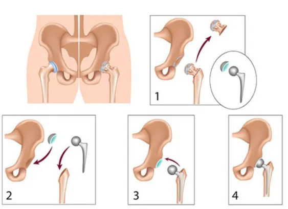
Total hip replacement needs to be performed when the hip-femoral joint is per-manently damaged and has to be replaced with a hip prosthesis. In this proce-dure, the head of the femur is removed to access the femoral canal and insert a

(13)

2 Chapter 1. Introduction

Figure 1.1: Anatomy of the hip joint. Source: www.corentec.com - hip anatomy

implant-stem which is then connected to an acetabular cup that goes inserted in the acetabulum of the hip bone (Figure 1.2).

In the current practice of THR, an increasing number of procedures are per-formed with cementless stems (Figure 1.3), especially when treating young patients with high activity level (Søballe, 1993; Holzwarth and Cotogno, 2012). This type of implant has shown to provide multiple advantages as opposed to cemented ones; first, cementless implants allow to avoid the introduction of cement in the organism of the patient that could generate the so-called cement disease, or polymethyl methacry-late debris, causing rejection reactions, premature loosening and other complications (Learmonth et al., 2007), they also help to match more properly the properties of the surrounding bone, thanks to the implementation of bioactive coatings and rough surface textures that cementless stems usually have incorporated to help enhance bone in-growth and fixation (Søballe, 1993; Søballe et al., 1992; Holzwarth and Co-togno, 2012; Karachalios, 2014). Among the most commonly used metal materials in orthopedic prostheses we can find: stainless-steel, cobalt-chrome, titanium and titanium alloy. Cementless hip prostheses made of a Ti alloy (Ti-6Al-4V) are char-acterized for having a high corrosive resistance, and has proven to be particularly

(14)

1.1. Context and motivation 3

Figure 1.2: Total Hip Replacement Scheme. Source: www.drugwatch.com - hip replacements

biocompatible in comparison with other materials. One of the advantages of this material is that its mechanical properties adapt well to those of cortical bone, which helps reduce non-anatomical bone remodeling caused by stress shielding (Søballe, 1993).

The use of a cementless implant involves a press-fit condition between the stem and the femur that is crucial for a proper fixation, and the survivorship and good function of the joint replacement (Karachalios, 2014; Ramamurti et al., 1997). Ob-taining a proper press-fit at surgery indicates that there is a good anchorage of the implant in the bone cavity (Karachalios, 2014; Ramamurti et al., 1997); this is a necessary conditions to obtain primary stability, which is defined as the me-chanical fixation of an implant achieved at the time of the surgery (Karachalios, 2014). Primary stability, is paramount for achieving bone in-growth, also known as the osseointegration process guaranteeing good functional outcomes (Albrektsson and Albrektsson, 1987; Viceconti et al., 2006) especially in the early post-operative period.

There are multiple debates regarding the threshold of bone-implant relative mo-tion that allows proper bone in-growth, it has been reported by multiple authors that there seems to be a relation between the magnitude of bone-implant motion and the type of interface tissue developed after surgery (Søballe et al., 1992; Bragdon et al., 1996). The formation of fibrous tissue is undesired since it is mechanically

(15)

Figure 1.3: Cementless hip stem without the femoral head -SPS Evolution Symbios. Source: www.symbios.ch

unstable (Søballe et al., 1992). To obtain a proper bony in-growth, the movement of the implant within the bone, also called "micromotion" ((Karachalios, 2014)), should not exceed 150 µm (Søballe, 1993; Bragdon et al., 1996).

1.1.2 THR broaching and bone properties

At the macrostructural level, bone is differentiated into two different types, cortical or compact bone, and cancellous or trabecular bone (Figure 1.4).

Cortical bone composes the external layer of all bones, with a dense structure of low porosity (porosity usually lower than 15%), presenting a compact appearance at the macroscopic level (Mitton et al., 2011).One complication that affects this

Trabecular bone is found in the inner parts of bone, and presents a highly porous sponge-like appearance, with a 3D structure made of connected plates and rods, known as trabeculae (Mitton et al., 2011).

For the implantation of a hip implant, it is necessary to open the femoral canal by removing the trabecular bone and leaving an open access for the implant to penetrate. This step of the surgery is known as the broaching procedure, for this the surgeon uses a set of broaching tools of different sizes that are introduced

(16)

pro-1.1. Context and motivation 5

Figure 1.4: Structure of trabecular bone (up) and cortical bone (bottom). Source: M. Granke. Multi-scale investigation of bone quality using ultrasound. PhD Thesis

gressively in a size-increasing manner until obtaining the desired size of the cavity for implanting the stem (Figure 1.5). It appears obvious to infer that this broach-ing process would have a non-negligible effect on the mechanical properties of the trabecular bone, which would most likely affect the bounding conditions in the inter-face zone between the bone and the implant. Mechanical tests of indentation have been widely used for characterizing the mechanical properties of bone at different structural levels (Oliver and Pharr, 2004).

On the other hand, it has been demonstrated that the bone mineral density of the bone can be associated to its elasticity through different empirical equations (Keller, 1994; Wirtz et al., 2000; Helgason et al., 2008; Auperrin, 2009). Specifically in our context of interest, the Hounsfield densities can be extracted from computed tomography (CT) scan images of the bone to make a mapping of the mechanical properties of the bone after broaching by making use of those relations.

The Hounsfield density is a quantitative parameter that can be extracted from the CT-Scan images of the bone of the patient; it is expressed in Hounsfield units (HU), and it corresponds to a linear transformation of a measure of the attenua-tion coefficient of the X-rays and a normalizaattenua-tion with respect to the attenuaattenua-tion coefficient of water. It is expressed by:

(17)

dHU = 1000 ×

µX − µwater

µwater

,

Where dHU, µX and µwaterare the Hounsfield density, the attenuation coefficient

of the X-rays in the material in question (bone), and the attenuation coefficient in water. For standard pressure and temperature conditions, the Hounsfield density in water is zero and the Hounsfield density in air is -1000 HU (Aamodt et al., 1999), while for the cortical bone is between 400 and 1000 HU (Shapurian et al., 2006).

Figure 1.5: Broaching tools (Symbios ) of different sizes used for THR.R

1.1.3 Preoperative Planning

THR is performed with the aim of recovering the biomechanical functionality of the hip joint when it’s damaged, for this a very precise work has to be done during the surgery to recreate the original anatomical configuration of the patient. In cementeless THR, the choice of the size and position of the implant for each specific patient is vital for obtaining the correct press-fit and primary stability (Reggiani et al., 2008; Holzwarth and Cotogno, 2012; Karachalios, 2014) previously described. The implantation of the stem in the bone and the evaluation of the level of anchorage is commonly assessed by the orthopedic surgeons in a rather empirical fashion. According to communications with an experienced orthopedic surgeon and limited literature reference (BEGUEC et al., 2015) a common practice is to use the sound of hammer blows as an indication of the quality of the press-fit between the implant and the bone. This implies that the stem size, position, and attainable stability is usually assessed empirically by the surgeon in the operating room with an inherent risk of error. For instance an underestimation of stem size may lead to pain, lower limb shortening or dislocation, whereas an overestimation may generate bone fractures and limb lengthening (Knight and Atwater, 1992; Sariali et al., 2012a).

(18)

Radiographs (X-rays) are used as a preoperative two-dimensional template for planning the surgeries, and anticipating prosthesis size and possible complications. This technique however, has proven to be highly dependent on the level of experience of the surgeon, and leads to prediction errors of size and position of the implant in approximately 50% of the cases when using cementless implants (Knight and Atwa-ter, 1992; Carter et al., 1995; González Della Valle et al., 2008; Sariali et al., 2012a) and originating problems such as lower limb discrepancy (Sariali et al., 2012a).

In order to assist the surgeons in making the correct selection of the prosthesis and plan the surgeries preoperatively, new tools are becoming available that allow to make a planning of the procedure more accurately, such as HipPlan and HipOP (Viceconti et al., 2003a; Sariali et al., 2009b, 2012a, 2016), this may in particular be of big help for the less experienced surgeons. Specifically, three-dimensionnal (3D) preoperative planning software, which are mainly based in anatomical compatibility techniques, make use of CT-Scan images of the hip joint of the patient and a 3D numerical model of the implant, allowing the surgeon to make a navigation with the digital model of the prosthesis. The surgeon virtually places the stem and the acetabular cup in the cavity of the femur and the acetabulum respectively, until finding the correct size and position for the implant, which is specified by a representation of the density of the bone projected on the surface of the stem’s model (HipPlan , Symbios, Yverdon-les-bains, Switzerland), (Figure 1.6). WithR

these tools, the surgeon anticipates the final position of the stem in the bone cavity after the insertion by successive hammer blows (Sariali et al., 2009b). More precisely, the surgeon needs to decide whether the regions of contact between the stem and the bone, for a given model and size of stem, can ensure a satisfactory anchorage by press-fit. However, the surgeon only has visual and geometrical arguments to make a decision and needs some training to take benefit of the 3D planning. This among others, is seen as one of the reasons the preoperative planning is seldom used in clinical practice while it may significantly help reduce failures, as explained below.

A study performed using the 3D preoperative planning software Hip-Op on the accuracy of CT-based surgical planning for THR as compared to traditional 2D templating planning (Viceconti et al., 2003a), shows that the accuracy of the se-lection of the size of the stem and the socket increased from 83% for the stem and 69% for the socket to 86% and 93% respectively. Demonstrating an improvement on the accuracy of the planning, specially when deformed anatomies are involved, and showing a high precision and accuracy specially for less experienced surgeons.

Sariali et al. have performed several studies on the accuracy of 3D preopera-tive planning using the HipPlan software. In a study to evaluate the accuracy of reconstruction of the hip using 3D preoperative planning and cementless implants (Sariali et al., 2009b), 223 patients with osteoarthritic hips were analyzed using the 3D planning tool. The post-operative restoration of the anatomy was assessed by

(19)

Figure 1.6: 3D preoperative planning - HipPlan.

CT and compared with the pre-operative plan, with accurate results in 86% of the cases for the acetabular component, 94% for the stem, and 93% for the neck-shaft angle. They conclude that the method appears to provide high accuracy, as the difficulties that can be found at the moments of the surgery can be anticipated and solved pre-operatively.

In another study (Sariali et al., 2009a) to determine 3D morphological data of the hip focusing on femoral offset (defined as the distance between the center of the femoral head and the femoral axis (Sariali et al., 2009a)) and using the software HipPlan, the mean femoral offset was found to be 2.2 mm greater than the 2D femoral offset values reported in the literature, the authors conclude that 3D planning software could allow an optimization of the planning process and the design of hip prostheses.

Given the potential that 3D planning tools seem to have for the improvement of THR, the interest for the advancement of techniques for these planning tools appears to be increasing in the last few years.

One study attempted to use anatomical compatibility and data set registration techniques for automated positioning of the hip implant based on predefined po-sitions from 3D preoperative plans done by surgeons, the method produced good results for implant positioning when compared to manual positioning done by an experienced surgeon (Viceconti et al., 2003b).

(20)

Another study proposed an atlas-based approach for automated 3D preoperative planning for THR (Otomaru et al., 2012). Statistical atlases were constructed from a number of 3D preoperative plans performed by experienced surgeons; based on distances map representing the preference of bone-implant contact patterns of the surgeon, 40 cases were evaluated utilizing the automated technique, and errors were measured as differences between the automated and a surgeon’s plan. By using the automated method positional and orientation errors were reduced as compared to other planning techniques, particularly 2D template methods.

1.1.4 Vibration Methods - Implant Stability

In this study we propose the use of vibration methods for the analysis of stability of cementless hip prosthesis during preoperative planning. In other words, we have combined 3D planning with a vibrational analysis to enhance the planning. Various studies have been carried out by multiple authors during the last few decades on the implementation of vibration methods perioperatively (during surgery) for the analysis of stability of hip prostheses and other types of implants, revealing promis-ing applications of this technique for stability assessment pre and perioperatively. We have identified two main research groups that have been consistent through out the years in the advancement of this technology and have inspired some of our study ideas, they are the team of Pastrav et al. from Leuven Engineering University College, Leuven, Belgium, and the team of Viceconti et al. from the University of Bologna and Rizzoli Orthopedic Institute, Bologna, Italy. The following presents a summary of some of the works of these and other authors:

1.1.4.1 Experimental studies:

Various experimental studies have been proposed with the goal of shedding light on the applicability of vibration methods for the analysis of stability of hip prostheses. Pastrav et al. (2009b) and Varini et al. (2010) proposed systems and protocols for perioperative assessment of stability of hip prostheses.

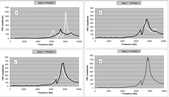
Pastrav et al. (2009b) developed a system to measure in-vivo the frequency re-sponse functions of the stem-femur system corresponding to successive insertion stages on the implant with the goal of detecting the insertion end-point of non-cemented and partially non-cemented hip stems. They observed that the higher mode numbers (frequency range 0-10 kHz) are more sensitive to the stability change com-pared to the lower mode numbers, in agreement with numerical studies Pastrav et al. (2009a), and also that during the insertion of the implant in the femur, the changes of boundary conditions and implant stability between different stages are reflected by the resonance frequency evolution (Figure 1.7).

(21)

Varini et al. (2010) presented a study focusing on an in-vitro validation of a de-vice to measure implant stability perioperatively based on vibration analysis. Fresh cadaver specimens and composite samples were used for the study. The device was composed by an excitatory piezoelectric system that delivered a controlled excita-tion to the prosthesis [1200-2000 Hz], and an accelerometer mounted on the host bone measured the transmitted vibration to identify resonance frequencies, which were measured immediately after press-fitting. Simultaneously a torque was applied to the implant and bone-implant micromotions were measured with the use of a displacement transducer. With this vibration technique they were able to discrim-inate between different levels of stability, concluding that the highest peak in the excitation range due to torque application is the best indicator of implant stability, and that when that shift is less than 5 Hz during the application of the torque, the residual micromotion after removal of the load was always less than 150 µm, which has been identified in other studies as the threshold for a correct implant anchorage (Søballe, 1993; Bragdon et al., 1996).

In terms of loosening detection techniques, Puers et al. (2000) developed an im-plantable telemetry system for the detection of hip prostheses loosening by applying vibration analysis techniques. With an accelerometer placed in the head of the hip prosthesis, they monitored the response of the femur-prosthesis system to mechan-ical sine wave vibrations applied by an electromagnetic shaker at the distal end of the femoral bone. The author claims satisfying preliminary results with cadaver experiments, although no specific data is reported.

Figure 1.7: Frequency response function graphs corresponding to successive insertion stages of a non-cemented stem. Each successive stage follows a hammer blow.

(22)

1.1.4.2 Numerical studies:

Qi et al. (2003) implemented a numerical modal analysis using finite element meth-ods and computer simulations to determine how much information a vibrational technique can reveal regarding the loosening of the femoral component of a total hip reconstruction. They computed and observed the first ten natural frequencies and mode shapes (Figure 1.8, right) of the implant-femoral model under free vi-bration, with hypothetical absence of contact portions at specific locations (Figure 1.8, left), and presented the interface failure size as a quantitative measurement of the femoral prosthetic loosening. They observed variations of the effect of interface failure (absence of contact) on the stiffness of the femoral component with different location and sizes of the failure zone, finding that higher modes are more sensitive to interface failure, and that the method was able to properly detect loosening when the size of interface failure was more than one-third of the length of the stem.

Figure 1.8: Example of hypothetical interface failures, 1/3 distal interface failure (left). First 6 vibration modes of the control model (right). Reproduced from Qi et al. (2003)

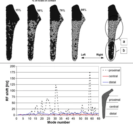
Pastrav et al. (2009a) performed a finite elements modal analysis on the hip stem-femur system under various contact situations (Figure 1.9, top) simulating different stages of the insertion of the implant in the bone’s cavity, and observed variations in modal shapes and natural frequencies. In agreement with Qi et al. (2003), their

(23)

results show that a shift to higher frequencies correspond to an increment of the implant-bone contact surface, with a more pronounced effect on higher modes. They also observed that the dynamic behavior is most influenced by proximal contact changes (Figure 1.9, bottom).

Figure 1.9: Top: Change of contact distribution: progressive increase of general contact (left); different contact areas in different zones; (a) proximal and central zones; (b) distal zone (right). Bottom: Resonance frequency shift plotted for proximal, central and distal contact increase (38-98%), free-free suspension of the implant-femur system. Reproduced from: Pastrav et al. (2009a)

In a similar study, Perez and Seral-Garcia (2013) determined the variations in the numerical modal analysis of a cementless hip prosthesis simulating different stages of the osseointegration process. Natural frequencies and modal shapes were observed under vibration for different bone and implant material properties and also different contact conditions at the bone-implant interface. It was found that as the osseointegration process evolved, increasing the contact surface and stiffness in the bone-implant interface, the values of the natural frequencies also increased in agreement with observations of Qi et al. (2003) and Pastrav et al. (2009a), and concluding also that higher modes and their corresponding resonance frequencies are more sensitive to contact conditions in the interface.

(24)

1.2. Enhancement of 3D planning 13

As evidenced in the aforementioned studies, vibration analysis has been consid-ered and proven to have good potential as a mean to assess primary stability of hip stems. It has been demonstrated that the vibrational behavior of the stem is mod-ified when the stem is progressively inserted into the femoral cavity by successive surgeon-controlled hammer blows. More precisely, resonant frequencies of the first vibration modes converge to plateau values as the stem’s end-point of insertion is reached.

For 3D planning purposes, Reggiani et al. (2007) showed that a finite element (FE) model built from the CT-scan of a cadaveric femur could predict the level of primary stability achieved for a cementless stem. Their analysis is based on the simulation of the quasi-static torsion of the stem and the computation of torsional micromotion. The model, which incorporates a finite element mesh of the bone and frictional contact conditions, is quite realistic but as a counterpart has several parameters and requires relatively large computational resources. Our hypothesis is that primary stability can be assessed during planning by resorting to a somewhat simpler model based on the modal analysis of the stem.

1.2 Enhancement of 3D planning

Even though currently available 3D preoperative planning tools represent an impor-tant step forward for the advancement of THR techniques, they are still in early stages of development. One critical limitation that has been identified in these tools is the lack of relevant mechanical criteria that is used to guide the surgeon during the planning. As it can be observed in Figure 1.6, the software only provides vi-sual information obtained from the levels of density of the bone in contact with the numerical object of the implant, but it does not specify the mechanical implications of the cartography observed, that is, what do those colors actually say about the global quality of the press-fit of the bone-implant interface?

The definition of this mechanical criteria is at the core of this thesis project, and represents an important part of the contribution of this work for the enhancement of 3D preoperative planning techniques.

In this thesis work, the technique that we propose is based on the implemen-tation of a finite element method for performing a modal analysis of the stem for the assessment of primary stability of cementless hip implants, with the purpose of determining numerical indicators that can be used to discriminate between stable and unstable cases during preoperative planning. In short, we introduce resonance three-dimensional planning (RP3D) as a mean to assess primary stability preoper-atively.

An exploratory preliminary study was performed using clinical data to identify from real cases common markers of stability discrimination. Then, in a study of

(25)

controlled cases those same markers served to identify the typical boundary con-ditions necessary to achieve stability. One advantage of our technique lays on its simplicity, since only the implant is included in the geometry of the finite element model (i.e no need to mesh the bone).

In the other hand we studied the effect of the broaching procedure on the bone, to this date this effect has not been defined and characterized, and any efforts towards the implementation of 3D preoperative planning techniques seem to be incomplete without a full understanding and consideration of the real contact conditions in the bone-implant interface, determined by the properties of the bone at the moment of the implantation, i.e. bone surface after broaching.

The existing 3D preoperative planning software make use of CT-Scan images of the patient before surgery, which evidently have not been through the broaching process yet. As a result, the planning obtained is based on a mere approximation of the actual contact conditions, since the real bone properties in the interface after broaching are not taken into account, this approximation may be far from reality depending on how important the effect of the broaching process on the bone surface is. On that account, it appears necessary to quantify the effect of the broaching process on the mechanical properties of the contact surface of the bone, to determine whether or not an approximation without taking into account the broaching effect is accurate enough for obtaining a realistic planning.

The potential of vibration methods for stability discrimination in THR has been established numerically and experimentally. Now, there is an interest for investigat-ing the usefulness of this technique in the specific context of preoperative planninvestigat-ing, and to establish the considerations related to the real boundary conditions in the bone-implant interface due to the effect of the broaching process.

1.3 Objectives of the thesis

• Introduce resonance three-dimensional planning (RP3D) as a mean to assess primary stability preoperatively; and evaluate the sensitivity and applicability of the method.

• Determine how, and to which extent, preoperative CT-Scan information can be used for RP3D. Define what is the relation between preoperative bone mineral density and the actual bone-implant contact.

1.4 Outline of the thesis

Chapter 2 introduces the finite element model, and numerical simulation consid-erations, taken into account for the vibrational analysis of the stem for stability

(26)

1.4. Outline of the thesis 15

discrimination.

Chapter 3 presents an exploratory preliminary study based on clinical cases, as our first attempt to use the numerical vibration technique for identifying discriminatory factors between stable and unstable cases from the modal response of the stem.

In Chapter 4 we present a fully developed vibrational finite element study based on controlled cases of bone-implant contact conditions for the definition of stability thresholds.

Chapter 5 is concerned with the characterization of the effects on bone properties of the broaching procedure by implementing image analysis techniques to measure bone mineral density variations on the µCT-Scan images of cadaver samples before and after broaching.

Chapter 6 presents a study of the mechanical properties of the bone by imple-menting an indentation mechanical testing on cadaver bone samples at the surface of the broached cavity.

(27)

(28)

Chapter 2 Numerical Model

2.1 Introduction - Finite Element Analysis (FEA)

This chapter is dedicated to present the numerical model and FEA methods imple-mented in the context of our study.

A finite element (FE) modal analysis was conducted on the software of numerical simulations and analysis Code Aster (Code_Aster, EDF R&D, license GNU GPL, http://www.code-aster.org) implementing the Sorensen method for modal compu-tation. The outputs of the computation are the modal frequencies and modal shapes calculated in the frequency range [0 − 21 kHz].

A .comm file is created, which contains the algorithm with the specifications of the FEA to be performed, including: FEA method, areas of affectation (nodes and elements to be affected), mechanical properties of the object, boundary conditions, stiffness matrix (corresponding in our case to the contact stiffness on the bone-implant interface) among other parameters depending on the desired outputs.

Salome-Meca (Salome-Meca, EDF Open Cascade, license GNU GPL, http://www.salome-platform.org/) was used to visualize the modal shapes. Code_Aster results were post-processed with custom Matlab (MATLAB Release 2015a, The MathWorks, Inc., Natick, Massachusetts, United States.) programs.

More detailed information regarding the FEA performed in each specific study will be presented in chapters 4, and 3.

2.2 Geometrical model

A finite element mesh was created for a cementless stem (SPS , Symbios, Yverdons-R

les-bains, Switzerland), see Figure 1.3. Meshes of two different sizes were created for each side, left and right, for a total of four meshes. Size C: height 11.5 cm, length 3.4 cm, and width 2.5 cm. Size D: height 12.2 cm, length 3.6 cm, and width 2.6 cm. The stem is a cementless anatomic model with a metaphyseal proximal fixation which is made of titanium alloy Ti6Al4V-Iso 5832-3, assumed isotropic and linear elastic, with Young Modulus 114 GPa, Poison ratio 0.34 and density 4500 Kg/m3. A CAO file (.ply format) of the stem, Figure 2.2, was provided by the manufacturer and used to create the FE mesh.

The CAO objects of the stem (provided by Symbios) contained small geomet-rical details (such as engraving) and could not be used as such to create a mesh. Therefore, the CAO file was first processed to remove small details which have a

(29)

18 Chapter 2. Numerical Model

negligible effect on the vibrational behavior in order to obtain a regular well con-ditioned mesh. Furthermore, in order to control the mesh density a parameterized geometry was created.

In order to do this, first, 15 cross-section contours were extracted from the CAO file (Figure 2.1). The contours selection process comprehends several steps since the nodes on the surface of the stem in the CAO file are not evenly distributed, which makes the extraction of the contours a little more laborious. To do this, three points per contour are selected directly on the surface of the object. With these three points the equation of the plane in which that contour is contained is obtained, then a tolerance value is manually assigned to each contour plane equation to include points that are located in adjacent planes of the CAO object and be projected on the plane of interest to fill the holes of areas where there are no points due to the uneven distribution of the original mesh (Figure 2.1). An interpolation is done to put all the points on the same contour line, to finally obtain a complete contour representative of the geometry of that part of the stem (Figure 2.2).

-50 50 0 70 60 50 40 30 20 10 0 -10 -20 -80 0 -70 -60 -50 -40 -30 -20 -90 -10 61 62 63 64 65 66 67 68 -23 -22 -21 -20 -19 -18 -17 -15 -10 -5 0 5 10 15 -8 -6 -4 -2 0 2 4 6 8

Raw contour 1, plane view

Raw contour 15, plane view Raw contours, ensemble

Figure 2.1: Visualization of the 15 contours in raw state, extracted from the CAO object. Left: ensemble of all 15 contours. Right: Plane view of contours 1 and 15.

Once the desired contour shapes are obtained, a new discretization is performed to obtain points evenly distributed over the contour by verifying consistency with the Pythagorean theorem, with the hypotenuse equal to the desired mesh element size (e). Then, the points are connected by lines to create a geometry file (.geo format), with the implementation of an algorithm adapted from a master’s thesis (Vallet, 2013), see Figure 2.3. This was then imported into the meshing tool GMSH (Geuzaine and Remacle, 2009) to create the mesh of the stem. For the obtained element size (e) the mesh consisted of ≈ 24000 degrees of freedom, and ≈ 22500 tetrahedral second order elements (Figure 2.4).

(30)

2.2. Geometrical model 19

Figure 2.2: Visualization of the 15 contours after interpolation and reorganization, represented over the original CAO object.

ï 10 ï 5 0 5 x 10ï 3 5 6 7 8 9 10 11 12 x 10 ï 3 x (cm) z (cm) ï 10 ï 5 0 5 x 10ï 3 ï 5 0 5 10 x 10ï 3 x (cm) z (cm) ï 10 ï 5 0 5 x 10ï 3 ï 6 ï 4 ï 2 0 2 4 6 8 10 x 10ï 3 x (cm) z (cm) Fit ï 10 ï 5 0 5 x 10ï 3 ï 6 ï 4 ï 2 0 2 4 6 8 10 x 10ï 3 x (cm) z (cm) (i) (ii) (iii) (iv)

�

x

�

y

Figure 2.3: Successive steps for the construction of the mesh of the implant from the CAO object: (i) Extraction of contour points from the CAO object (ii) Interpolation of the contour (iii) Testing of points verifying Pythagoras’s theorem, with hypotenuse equal to the desired element size (iv) Cloud of equidistant points forming the origin contour that is saved into a file format to be interpreted and processed on gmsh

(31)

Contours of the .geo ﬁle

Mesh of the stem produced on GMSH

Figure 2.4: Left: Illustration of the contours saved into a .geo file format to be interpreted and processed on gmsh. Right: Mesh of the stem obtained on gmsh from the .geo file.

2.3 Mesh

In order to determine the appropriate mesh size, a convergence study was performed on a cantilever beam for which an analytical solution of the eigen-modes is available. For this convergence study we took into account the cantilever beam theory and Newton’s equation. Three different boundary condition (BC) configurations were considered for the cantilever beam, embedded-free, double-embedded, and free conditions.

The cantilever beam presented the following geometrical characteristics: 5×0.2× 0.1 cm (L × h × b). And mechanical properties: E =210 GPa (Young’s Modulus), G=79.3 GPa (shear modulus); ρ=7800 Kg/m3(volumetric mass). The second order mesh had 9286 degrees of freedom, and 5024 tetrahedral elements (Figure 2.5, a).

The eigen-modes of bending, torsion, and longitudinal motion were evaluated for each BC configuration on Code Aster. We selected a number of elements per wave-length of 16, which satisfies the Courant-Friedrichs-Lewy (CFL) condition, with an average error of 0, 093% between the FE solution and the analytical result for the first seven eigenmodes, with the embedded-free configuration (Figure 2.5, b); this corresponds in our study to a characteristic element size of e = 2 mm.

2.4 Boundary Conditions (BC)

In our modal FEA studies, the boundary conditions are given by the stiffness in the bone-implant interface zone, which is simulated by springs attached to nodes on the

(32)

2.5. Registration of HU densities on the mesh 21

(a) Visualization of the mesh of the beam cantilever on GMSH, with the fi-nal FEM characteristics selected from the convergence study

wavelength per element (lambda/delta)

10 15 20 25 30 35 40 45 50 Frequency Error(%) 0 0.05 0.1 0.15 0.2 0.25 0.3 mode1 mode2 mode3 mode4 mode5

(b) Graph wavelength per element Vs. Frequency error, for the first five modes of the modal analysis of the beam can-tilever.

Figure 2.5: Beam cantilever convergence study

surface of the stem (Figure 2.6). Some nodes are affected by this stiffness, and the rest of the nodes are free.

The reaction force on node i of the stem writes:

Fi = ki∗ ui (2.1)

where ki is the stiffness of an individual spring and ui is the displacement vector

of the node i.

The variable stiffness K (the equivalent stiffness of the whole contact surface) is applied perpendicularly to the contact surface of the mesh of the stem, and dis-tributed homogeneously over the surface in question by adjusting k_i. A study was done with a simple beam cantilever to verify that the stiffness is in fact distributed homogeneously on the surface and not applied individually to each node.

Different approaches of this same method are used for the FE studies in Chapters 4, and 3, for representing the interface stiffness that corresponds to each study.

2.5 Registration of HU densities on the mesh

The current 3D preoperative method is a black-box, the relationship between what happens in the bone-implant interface and the visual information of the HU is unknown. We have started to work on the creation of a color map with our own mechanical criteria directly from the preoperative planning.

From the 3D planning we obtain a cloud of points with an associated HU density, in order to convert these HU densities into boundary conditions for the FEA, these density values need to be associated to its corresponding node on the mesh.

(33)

k

i

Figure 2.6: Springs stiffness effect attached to the nodes of the stem.

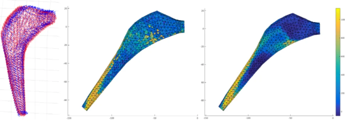
Different techniques were proposed for this association of values to each node, among them: the values contained in a normal of a certain length on each node, the values within a certain radius, and the nearest value, see figure 2.7 for an exam-ple; we observe how the distribution changes according to the registration method implemented. One difficulty for the application of these methods is that the mesh obtained from the CAO object of the stem and the cloud of points obtained from the 3D planning are expressed in different coordinate systems, and a transforma-tion matrix is needed to make the right registratransforma-tion, this matrix defined in the 3D planning software is not easily accessible. For the moment this registration is done manually.

Figure 2.7: Registration of HU values from the 3D planning on the FE mesh. Left: Illustration of normals defined on each node for association of HU values. Middle: ex-ample of an HU density distribution with the "nearest value" method. Right: exex-ample of an HU density distribution with the "nvalues within a radius" method

(34)

Chapter 3 Modal analysis of clinical cases

3.1 Introduction

In this chapter we present an exploratory study dedicated to assess the applica-bility and advantages of implementing numerical modeling methods to analyze the vibrational behavior of a cementless hip implant for the determination of primary stability in preoperative 3D planning. Based on a few clinical cases, and making use of the numerical model presented in 1; we present the application of a modal analysis of the stem, specifically modal frequencies and modal shapes, subjected to boundary conditions defined by the contact with the surrounding bone in the femoral cavity, obtained from CT-Scan information of a 3D planning.

As presented in chapter 1, multiple studies ((Qi et al., 2003; Pastrav et al., 2009a,a; Varini et al., 2010; Perez and Seral-Garcia, 2013), among others) have been presented proposing different vibration techniques for the analysis of stability in THR, both preoperatively and perioperatively. These experimental and numerical works propose various methods for the discrimination of stability defined as a func-tion of the frequency response of the bone-implant system, and the mode shapes. It has been demonstrated that a shift towards higher frequencies is related to a better stability. Furthermore, these studies have shown how this enhancement of stability is due to an increase in the contact surface and the quality of the anchorage of the implant in the femoral cavity.

Our approach has two main advantages which shape the originality of this work. Firstly, we associate the HU densities from CT-Scan images of the bone with stiffness values, this allows to implement a simple model which involves attaching springs to the contact area of the stem with their corresponding stiffness. This way we simulate the effect of contact with the bone without having to include the bone in the geometrical model. And second, we establish a relation between indicators of instability from the numerical analysis and clinical indicators of unstable patients (i.e. patients in pain post-surgery).

Our hypothesis is that the modal analysis, namely modal frequencies and modal shapes, of the implant under boundary conditions obtained from the preoperative planning can serve to discriminate stable and unstable cases.

(35)

24 Chapter 3. Modal analysis of clinical cases

3.2 Materials and Methods

Figure 3.1 displays the main steps that were followed for the completion of this exploratory numerical study. First, CT-Scans of each patient were acquired before the surgery, the CT-Scanner was calibrated to maintain consistency with the scans after surgery. The preoperative CT-Scan images were used for the 3D preoperative planning performed by the orthopedic surgeon. These plannings were used as a reference for performing the THR surgery by the same surgeon. Post-surgery 3D plannings of six patients were used for the numerical study. These post-surgery plannings were used to superpose and verify the position planned with the preop-erative planning CT-Scan images of the patient, and make sure that the planned position was achieved. Also, these plannings are done after the surgery to run the numerical study with the bone-implant conditions obtained after the surgery is per-formed. The finite element modal analysis was done on Code ASTER following the method described in chapter 2.

3D Pre-operative

Planning

THR Surgery

Vibration

FE Analysis

3D Post-operative

Planning

Discrimlnation of stable and unstable and comparisons with clinical diagnosis

Diﬀerentiation of stable and unstable cases from clinical observations Peformed by the orthopedic surgeon

Preoperative

CT-Scans

Calibrated for consistency with posteoperative scans

Peformed by the orthopedic surgeon following the preoperative planning

Post-operative

CT-Scans

Calibrated for consistency with preoperative scans

Figure 3.1: General scheme with the different steps of the procedure

Presentation of study cases

The six cases (Hôpital Pitié Salpètrire, Orthopedic Service Department) were se-lected by the surgeon and classified as stable or unstable, by taking into account common clinical parameters, such as the presence of pain, limping, difficulties to switch from sitting position to standing position, or the inability to walk. The first

(36)

3.2. Materials and Methods 25

group (stable) exhibits a good osseointegration of the implant in the bone three months after the operation, while the second group (unstable) is formed by patients for whom the implant did not attain the stability condition as observed several months after the surgery.

The first group (patients A, B and C) correspond to a good osseointegration and a satisfactory implant-femoral stability, while the second group (patient E and F) present unstable implants with an insufficient level of anchorage of the implant in the femur. Finally, patient D was classified as having a good implant stability but presenting post-surgery pains. The six plannings are presented in table 3.1.

Patient A - stable Patient B - stable Patient C - stable

P3D

Patient D - stable with pain Patient E - unstable Patient F - unstable

P3D

Table 3.1: Images taken from the postoperative three-dimensional plannings (P3D) of patients A - F. The plannings of patients A, B, C and D correspond to stables prostheses, with presence of pain for patient D, the plannings of patients E and F correspond to unstable prostheses.

It should be noticed that patients A, B, C, D and F were operated with the same prosthesis model SPS modular (Symbios), size C; left side for patients A and D,R

and right side for B, C and F. Patient E was operated with a size D implant, right side.

Extraction of boundary conditions from the 3D planning

In this chapter we deal with the issue of converting Hounsfield density values of the bone in contact with the stem obtained from CT-Scan images of the patients in the planning, into a physical parameter that simulates the effect of the contact conditions in the bone-implant interface. For this, we apply the following reasoning, with the introduction of the implant into the femoral canal, a displacement of the

(37)

bone is imposed by a force exerted by the implant. The relation between this force and displacement is given by the apparent stiffness of the bone-implant interface. Hence, the physical parameter we search to convert the Hounsfield values into, is nothing but the contact stiffness in the interface.

From the work of Auperrin (2009) we obtain an equation to relate the Hounsfield density measured by X-rays and the volumetric mass of the bone. This relation is given for a volumetric mass equivalent to those we deal with in our study.

ρ = 0.0009dHU+ 0.8336 (3.1)

with ρ the volumetric mass, and d_HU the Hounsfield density.

In multiple studies it has been established that the Young’s modulus can be related to an apparent volumetric mass of the bone (Keller, 1994; Wirtz et al., 2000; Helgason et al., 2008). For this study the following relation was implemented:

E = 10.5 × (0.55ρ)2.29 (3.2)

Where E (GPa) and ρ (g.cm−3) are the Young’s modulus and the apparent volu-metric mass of the bone, respectively. This expression was obtained from the studies of Keller (1994) regarding relations between elastic properties and the volumetric mass of the femur.

With equation 3.2 we can calculate a local Young’s modulus for different zones of the prosthesis associated to different HU values. It follows that, for a determined thickness of the femoral bone e, a stiffness K can be obtained for different zones of contact, by implementing the following equation:

K = EHU×

S

e (3.3)

with K (N.m−1) the equivalent stiffness (see relation with equation 2.1 in chapter 2), E the Young’s modulus (Pa), S (m2) the corresponding area of the contact zone in question, and e the considered thickness in the bone-implant interface.

Equation 3.3 is derived from the following reasoning:

     F = k × x σ = E × ε ⇒          σ = F S ε = x e ⇒        E × ε = k × x S E × x e = k × x S ⇒ k = E ×S e

with F an applied force, on an element of length e, and surface S, causing a displacement x, originating an strain ε, and a stress σ.

(38)

3.2. Materials and Methods 27

Definition of contact surfaces

The 3D preoperative planning tool that we used (HipPlan, Symbios) allows to ex-tract the values of the Hounsfield density of the bone in contact with the implant from the preoperative QCT scan of each patient.

On the 3D planning every point on the surface of the implant is associated to a value of Hounsfield density.

A linear scale of Hounsfield densities is established, first a lower threshold of 400 was defined for the HU densities, which corresponds to the minimum HU density of cortical bone which was set in the range of 400 to 1000 (Shapurian et al., 2006). The points of the surface of the implant associated to HU densities below 400 would be considered as free of contact.

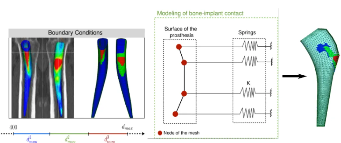
The Hounsfield densities are converted into volumetric masses with the equation 3.1. Then a scale of volumetric mass is established by defining three different ranges as shown in Figure 3.2 (left), which correspond to the assumed level of contact between the prosthesis and the bone, low contact in blue, medium contact in green, and high contact in red.

These three ranges of volumetric mass, for different contact areas are defined as follows: D = max(ρ) − min(ρ) ,     

ρblue∈ [min(ρ) ; min(ρ) + D/3] ,

ρgreen∈ [min(ρ) + D/3 ; max(ρ) − D/3] ,

ρred∈ [max(ρ) − D/3 ; max(ρ)] ,

These three ranges of volumetric mass allow to define three groups of points on the surface of the implant corresponding to three levels of contact (Figure 3.2, left). The volumetric mass of one zone corresponds to the average of the volumetric masses of the points of the associated range. The local values of stiffness for each zone are then calculated by using the equations 3.2 and 3.3.

The proposed contact model consists of attaching one spring representing a local stiffness (Figure 3.2, middle) to each one of the nodes of the mesh located on the three contact zones (Figure 3.2, right).

To calculate the area of each of the three contact zones, we calculate the indi-vidual areas of each surface element of each contact zone. These are computed as the area of a triangle formed by one node and the two closest neighbor nodes, then we make the summation of each individual triangle in each contact zone to obtain the total area of each surface.

Finally, with each total area for each zone S, the Young’s modulus E calculated for the corresponding zone, and assuming the unit value for the thickness of the bone e, the equivalent stiffness keq of each contact zone is obtained.

(39)

Figure 3.2: Left: Contact zones defined of the prosthesis with a 3D planning. Middle and Right: Bone-implant contact modeling principle.

3.3 Results

In table 3.2 we present the modal shapes and modal frequencies for the first five eigen-modes for one stable patient and one unstable patient, both with implant size C, in a frequency range [0 : 20] kHz. Two of the stable patients (A and B) presented a total of 5 and 7 modes respectively, and the unstable patients (E and F) a total of 7 modes and 9 modes, respectively. The frequencies for the stable patients go from around 2-18 kHz, while for the unstable patient the frequencies range from around 2-16 kHz. The range of frequencies and the number of modes seem to present very variable patterns for stable and unstable cases. This is observed for all the 6 patients that we studied.

The information contained in the modal shapes is richer (see images in Table 3.2). For the unstable patient the modal shapes show a proximal bending, particu-larly in modes three and four, indicated by the variation of color on the top of the implant (not blue). For the stable patient the obtained modal shapes do not display this proximal bending. Similar patterns were observed in the other studied cases, with some exceptions in some of the patients were the modal shapes did not follow that pattern (see appendix A).

3.4 Discussion

The appearance of a stem bending mode concentrated on the proximal part seems to be the signature of an undesired fit, and as a result of bad primary stem stability. These results are coherent with the clinical experience, that indicates that excessive proximal motion of the stem is associated with a bad fit of the implant. Based on this preliminary results, and having found certain patterns of stability discrimination (presence of proximal bending) we have considered of importance to measure and

(40)

3.4. Discussion 29

Number of Eigen modes

Modes 1 2 3 4 5

A 5 8110 10525 11189 16213 17918 Hz

F 9 2357 2940 7418 9271 16137 Hz

Table 3.2: Modal shapes of the first five modes of two patients of the study, as well as the number of modes and modal frequencies in the frequency range [0 : 20] kHz. Proximal bending modes indicated by variation of color at the top of the implant (not blue).

characterize the effect of the magnitude of the contact stiffness and the size of the area on which it is distributed, to establish stability thresholds that can be used as a reference in preoperative planning. Furthermore, we consider crucial to be able to measure this proximal motion in the modal shapes with a numeric value, for this we have proposed to calculate the elastic potential energy ratio of the proximal part of the stem. These ideas are explored and presented in Chapter 4.

Our method applying local stiffness values through the use of springs to emulate the effect of the contact between bone and implant is a simple technique for running numerical simulations. However, one limitation is that in our analysis we consider a thickness e equal to the unit for obtaining the equivalent stiffness k_eq of each contact zone. The effect of the actual thickness is unknown, in fact even the physical definition of this thickness represents a challenge. With the goal of finding possible answers to these questions, in Chapter 6 we investigate a little further and discuss different considerations related to this thickness and its complexity.

Another limitation of this first exploratory study is that only six patients were analyzed. The method needs to be implemented on a larger group of patients to assess consistency of the observation.

(41)

(42)

Chapter 4 Modal analysis of controlled cases

The material presented in this chapter was submitted for publication in the journal "Medical Engineering Physics". Title of the article: "Modal analysis for the assessment of cementless hip stem primary stability in preoperative THA planning".

Ideally, a THR 3D planning software should provide a clear indication of the expected primary stability for a given stem in a given femur. In order to achieve this, a patient-specific mechanical analysis of stem stability must be done. Several factors play an important role in the press-fit condition of a cementless implant in THR, which ultimately define the primary stability. Among these factors, the contact zone size (CZS) and the apparent stiffness of the bone-implant interface are critical. This stiffness is found to be highly variable in patients, which must be taken into account in the planning. This can be achieved by using the densitometric information in the CT-scan which provides an indirect measure of stiffness (Helgason et al., 2008).

This chapter elucidates the relationships between the modal response of a hip stem (modal frequencies and modal shapes) and the boundary conditions on the stem in terms of area of contact zone (CZS) and the apparent stiffness at the bone-implant interface. This work is based on the hypothesis that variations in CZS and apparent stiffness are reflected in the modal behavior of the stem and that the latter converges to specific patterns characteristic of a stable stem as CZS and interface stiffness increase. If this hypothesis is true, a patient-specific modal analysis in the framework of the 3D planning could potentially discriminate between stable and unstable stem positions.

4.1 Materials and Methods

This chapter is dedicated to describe a study based on a finite element (FE) modal analysis of a cementless stem (SPS size C, length 120 mm, Symbios, Yverdons-les-R

bains, Switzerland) and its implementation to assess the effect of CZS and contact stiffness. Implementing the FE modeling methods using the software Code Aster, as described in chapter 2.

In order to evaluate the effect of the size of the contact area between bone and the stem, four different CZS of surface elements were defined on the surface of the stem mesh (Figure 4.1, Left): Small (400 elements ≈ 5cm2), Medium (800 elements

(43)

32 Chapter 4. Modal analysis of controlled cases

≈ 10, 5cm2_{), and Large (1200 elements ≈ 15, 6cm}2_{), a fourth intermediate CZS was}

included later for verification (SM, 600 element ≈ 7, 5cm2). The CZS’s positions and shapes were defined by an experienced orthopaedic surgeon, by taking into account the typical contact patterns that are observed in common clinical cases when a 3D preoperative planning is performed (Sariali et al., 2012b).

K Springs Nodes

Figure 4.1: Left: Large, Medium, and Small contact zones represented on the stem. Right: springs stiffness effect attached to the nodes of the stem.

The stiffness of the bone in contact with the stem is simulated by springs at-tached to each node of the contact zone surface (Figure 4.1, Right), as described in chapter 2, equation 2.1. The apparent stiffness K of each contact zone was chosen to range between 101− 1010 _{N/m which accounts for the whole spectrum of}

reason-able stiffness values. The apparent stiffness K is distributed evenly on the contact surface by adjusting k. Free conditions (no contact, i.e. k = 0) vibration modes were also computed for reference.

The FE modal analysis was conducted with Code Aster (Code_Aster, EDF R&D, license GNU GPL, http://www.code-aster.org) implementing the Sorensen method for modal computation. The outputs of the computation are the modal frequencies and shapes calculated in the frequency range [0 − 21 kHz].

4.2 Data Analysis

The number of modes in the range [0 − 21 kHz] and the frequencies and shapes of the first five modes were investigated with respect to contact apparent stiffness and contact area.

Similarities between modal shapes were quantified with the modal assurance cri-terion (MAC), a quantity which is used extensively in structural vibration analysis. The MAC is a scalar constant between 0 and 1 that relates the degree of similarity (collinearity) between two modal vectors (shapes) (Allemang, 2003). For each mode of number n (n varies typically between 1 and 5 in the present study), the MAC was

en fr

HAL Id: tel-01596018

https://tel.archives-ouvertes.fr/tel-01596018

Characterization of the bone-implant interface and

numerical analysis of implant vibrational behavior for a

mechanics based preoperative planning of total hip

arthroplasty

Andres Rondon

To cite this version:

Université Pierre et Marie Curie, Paris 6

Thèse de Doctorat

Andres Rondon

Acknowledgments

Abstract

Keywords

Résumé

Mots-clés

Contents

Chapter 1

Introduction

1.1

Context and motivation

1.2

Enhancement of 3D planning

1.3

Objectives of the thesis

1.4

Outline of the thesis

Chapter 2

Numerical Model

2.1

Introduction - Finite Element Analysis (FEA)

2.2

Geometrical model

�

x

�

y

2.3

Mesh

2.4

Boundary Conditions (BC)

2.5

Registration of HU densities on the mesh

k

Chapter 3

Modal analysis of clinical cases

3.1

Introduction

3.2

Materials and Methods

3D Pre-operative

Planning

THR Surgery

Vibration

FE Analysis

3D Post-operative

Planning

Preoperative

CT-Scans

Post-operative

CT-Scans

3.3

Results

3.4

Discussion

Chapter 4

Modal analysis of controlled cases

4.1

Materials and Methods

4.2

Data Analysis