Computational algorithms for adaptive robot control

ADAPTIVE ROBOT CONTROL

by

Guinter Dieter Niemeyer

B.S., Technische Hochschule Aachen, (1986) SUBMITTED TO THE DEPARTMENT OF AERONAUTICS AND ASTRONAUTICS IN PARTIAL

FULFILLMENT OF THE REQUIREMENTS FOR THE DEGREE OF

MASTER OF SCIENCE IN AERONAUTICS AND ASTRONAUTICS at the

MASSACHUSETITS INSTITUTE OF TECHNOLOGY February 1990

Copyright © Massachusetts Institute of Technology, 1990. All rights reserved.

Signature of Author .

Depaieet of Aeronautics and Astronautics January 25, 1990

Certified by

Accepted by

Professor Jean-Jacques E. Slotine Thesis Supervisor D artment of Mechanical Engineering

'1. )

WASSACHUSETTS INSTITUTE OF TECHNnt fGY

FEB •2 6

1990

VProfessor

---ADAPTIVE ROBOT CONTROL

by

Giinter Dieter Niemeyer

Submitted to the Department of Aeronautics and Astronautics on January 25,

1990 in partial fulfillment of the requirements for the degree of Master of Science

in Aeronautics and Astronautics.

Abstract

Effective adaptive controller designs potentially combine high-speed and high-precision in

robot manipulation. Furthermore, they can considerably simplify high-level programming

by providing consistent performance in the face of large variations in loads and tasks.

Globally convergent adaptive manipulator controllers have recently been developed for this

purpose. However, computational complexity has so far restricted their applicability to

manipulators with few degrees-of-freedom.

This work presents a new recursive algorithm, which effectively implements the simple, yet

globally tracking-convergent, adaptive sliding manipulator controller. To further improve

efficiency, a procedure is derived to select and evaluate a minimal set of inertial parameters

of the manipulator. Since many tasks require direct cartesian control, the algorithm is

subsequently expanded to handle cartesian data hi real-time and possibly exploit kinematic

redundancies. Finally, the application to constrained motion is discussed, introducing

impedance control features to guarantee stable contacts to arbitrary passive environments.

The complete system allows the effective use of adaptive strategies on multi

degree-of-freedom manipulators for a variety of tasks.

The developments are implemented and illustrated experimentally on a four

degree-of-freedom articulated robot arm and suggest a wide range of application beyond adaptation to

grasped loads.

Thesis Supervisor: Professor Jean-Jacques E. Slotine

I wish to express my deepest gratitude to my advisor, Professor Jean-Jacques Slotine.

He was a constant source of support, ideas, and excellent guidance and truly brought the

project to life.

Special thanks go to Professor Kenneth Salisbury and Dr. William Townsend, who

allowed me to use their truly fine manipulator and provided many stimulating discussions

and much encouragement. Also many thanks to Brian Eberman and Sundar Narasimhan,

who helped in the software implementation and were always full of suggestions.

I furthermore deeply appreciate the many friendships I have found here: My

long-time office-mates Andre Sharon, Ted Clancy, Harvey Koselka, and Hyun Yang, the

members of the Nonlinear Systems and Whole Arm groups, the Martin Design Center and

the Artificial Intelligence Laboratory. They all provided numerous pieces of helpful advice

and comments and made this time thoroughly enjoyable.

I also gratefully acknowledge the support from the H.A. Perry Foundation, as well as

partial support by the MIT Seagrant Office and Grant 8803767-MSM from the National

Science Foundation. Development of the arm and control hardware was supported by

Grants N00014-86-K-0685 and N00015-85-K-0214 from the Office of Naval Research.

Finally, I am most grateful to my family, who supported and encouraged my work in

any way they could and, I am sure, without whom I would not be here today.

Abstract

2

Acknowledgments

3

'Fable

of Contents

4

List

of

Tables

7

I.

Introduction

8

2.

Direct Adaptive Sliding Control

II

3.

Recursive Implementation

15

3.1 The Definitions of Spatial Quantities 17

3.2 The Relation of Joint and Link Inertia Matrices 18

3.3 Expressing the Coriolis Matrix 20

3.4 The Gravity Vector 24

3.5 Feedforward of the Inertial Forces 25

3.6 Adaptation Law for Inertial Parameters 26

3.7 The Complete Recursive Algorithm 26

3.8 Comparison to Newton-Euler and Walker Algorithm 28

3.9 Closed Kinematic Chains 29

4. Minimal Parameterization

30

4.1 Parameter Redundancies for Two Consecutive Links

31

4.2 Parameter Transfers through Rotational Joints

38

4.3 Parameter Transfers through Translational Joints

40

4.4 Parameter Reductions for Links with Restricted Motion

40

5. Cartesian Implementation

42

5.1 On-Line Inverse Kinematics ₄₃

5.2 Redundancy Solution 45

5.3 Implementation Aspects of Inverse Kinematics 46

6.

Applications to Constrained Motion

48

6.1 The Basic Passivity Concept 49

6.2 Passivity Interpretation of the Adaptive Controller 50

6.3 Adaptive impedance control ₅₃

7.

Experimental Results

₅₆

7.1 The Experimental Setup ₅₆

7.2 A Comparison between P.D. and Adaptive Control 60

7.3 Cartesian Control Experiments ₆₃

7.4 Whole Arm Experiments ₆₃

Appendix

A. The Spatial

Vector

Notation

₆₅

A. 1 The Spatial Vector Definition ₆₆

A.3 Reference Frame Transformations 68

A.4 The Spatial Inertia Matrix 69

A.5 The Dynamics of an Arbitrary Rigid Body 71

Appendix B. Evaluating the Link Force Coefficients 72

Appendix C. The Implementation Code 78

C. I Type and Variable Definitions 78

C.2 Controller Recursive Routine 80

C.3 Adaptation Recursive Routine 84

Figure 3- 1:

Figure 4-1:

Figure 6-1:

Figure 6-2:

Figure 6-3:

Figure 6-4:

Figure 6-5:

Figure 7-1:

Figure 7-2:

Figure 7-3:

Figure 7-4:

Figure 7-5:

Geometric Interpretation of Summations

Two consecutive links connected by a rotational joint

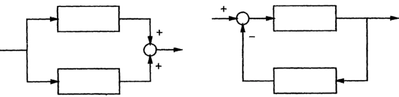
Negative feedback and parallel connections maintaining passivity

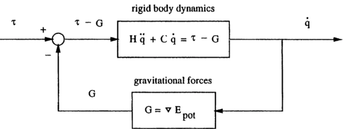
Passive Interpretation of a rigid manipulator

Open versus closed loop passive mapping of the manipulator

Passivity interpretation of the adaptive controller

Complete control system for constrained motion

The WAM manipulator

The coordinate frames of the WAM manipulator

Joint Tracking Errors q (in degrees)

Joint Torques z (in N.m.)

Cartesian Tracking Errors i'(t) (in cm)

3.2

4.1

6.1

6.2

6.2

6.2

6.3

7.1

7.1

7.2

7.2

7.3

Table

_{3-1: Complete Equations for the Recursive Implementation of the Direct}

_3.7

Adaptive Controller

Table

4-1:

Evaluation of 61

4.1

Table

4-2: Evaluation of

vk-

x S1

+ dk

x

kI

81

vk-1

d

4.1

Table

4-3: Upwards Transformation

of a Spatial

Inertia Matrix

4.1

Table

_{4-4: Downwards Transformation of a Spatial Inertia Matrix}

_4.1

Table

4-5: Transformation

of

the inertia parameters for rotational joints

4.2

Table

4-6: Transformation

of

the inertia parameters for translational joints

4.3

Table 7-1: Denavit-Hartenberg Parameters of the WAM manipulator

7.1

Table

7-2:

The

necessary

inertial

pannaters of the WAM manipulator

7.1

Table B-I:

Evaluation

of

R

i,

B

Table B-2: Evaluation of w x R

v

+

v x

i w + R

w

x

v

B

Table

B-3:

Analytic

functions for the individual force coefficients

B

Table B-4:

Velocity combinations for the force coefficient evaluation

B

Introduction

Adaptive control has been extensively studied, and several globally convergent

controllers have been derived for linear time-invariant single-input single-output systems.

Recent developments (for example [Slotine and Li, 1986], [Craig, Hsu, and Sastry, 1986],

[Middleton and Goodwin, 1986], [Hsu,

et

al, 1987], [Sadegh and Horowitz, 1987], [Bayard

and Wen, 1987], [Koditschek, 1987], [Slotine and Li, 1987a-e], [Li and Slotine, 1988],

[Walker, 1988]) have been able to derive adaptive manipulator controllers with similar

global convergence properties. This represents an important extension of adaptive control

to a class of nonlinear multi-input systems.

Such adaptive manipulator controllers

potentially provide consistently high performance in the face of large variations of loads

and tasks. Furthermore, this performance is achieved without requiring increased actuator

bandwidth.

A simple, yet globally tracking-convergent, direct adaptive sliding manipulator

controller was developed in [Slotine and Li, 1986] and demonstrated experimentally in

subsequent work [Slotine and Li, 1987b].

Though the controller provides excellent

performance and robustness properties, it application is currently limited by the computational burden of the nonlinear control and adaptation laws. Existhig recursive

algorithms are rendered useless as they do not match the nature of the controller.

The central part of the work presented here develops a new recursive algorithm to effectively implement the adaptive manipulator controller of [Slotine and Li, 1986]. This allows the application to multi degree-of-freedom manipulators, which so far have been excluded from the advanced control concepts.

An additional increase in computational efficiency can be achieved with the use of minimal parameter sets. This work also presents a procedure for selecting such minimal sets and evaluating the involved parameters. It is applicable to all joint types and kinematic structures and presents a more practical altemative to existing theoretical results ([An, Atkeson, and Hollerbach, 1985], [Khosla and Kanade, 19851, [Mayeda, 1988]).

Since many interesting tasks can be addressed with direct cartesian control, this work proceeds by extending the recursive algorithm to handle cartesian data in real-time. It thus provides a cartesian implementation of the adaptive controller. To handle redundant manipulators, a pseudo-inverse method is used with nullspace minimization of a joint position norm. On the basis of this cartesian implementation, the application to constrained motion is then examined. In particular, impedance control features are introduced to guarantee stable contacts with arbitrary passive environments. The complete system then allows the effective use of adaptive strategies on multi degree-of-freedom manipulators for a large variety of tasks.

The developments are implemented and illustrated experimentally on a four degree-of-freedom articulated robot arm. A comparison between P.D. and adaptive controller clearly demonstrates the improvements caused by the adaptation process. Further

experiments also suggest a wide range of application beyond the adaptation to grasped loads.

Following a brief review of the direct adaptive controller of [Slotine and Li, 1986] in Chapter 2, Chapter 3 presents the recursive algorithm for the implementation. The minimal parameter sets are derived in Chapter 4, after which cartesian implementation and application to constrained motion are discussed in Chapters 5 and 6 respectively. Finally the experimental results are detailed in Chapter 7.

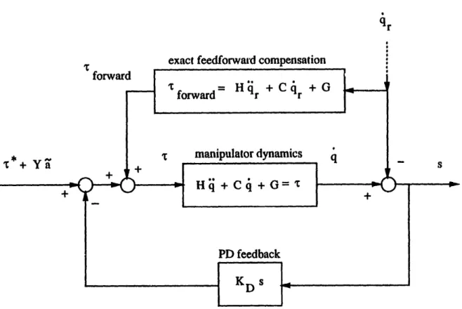
Chapter 2

Direct Adaptive Sliding Control

The direct adaptive sliding controller considered in this thesis was originally developed and later experimentally verified in [Slotine miand Li, 1986, 1987a]. It is applicable to all rigid manipulators, regardless of kinematic structure, and briefly summarized in the following.

In the absence of friction and other disturbances, the dynamics of an n degree of freedom rigid manipulator (with the load considered as part of the last link) can be written as

H(q) q + C(q,q) q + G(q) = s (2.1)

where q and u are the nx I vectors of joint displacements and applied joint torques (or forces) respectively. H(q) denotes the nxn symmetric positive definite (s.p.d.) manipulator inertia matrix, C(q,q) q is the nxl vector of centripetal and Coriolis torques, and G(q) gives the nxl vector of gravitational torques. A friction model can be added to the above dynamics, using e.g. D, sgn(4) and D,, q as the nxl vectors of static (Coulomb) and

viscous friction torques. Note that the sign operator sgn(.) is performed independently in

each component, and the matrices D

and D,, are diagonal positive definite (or

semi-definite). Including friction, the manipulator can thus be modeled as

H(q) q + C(q,qi) q + G(q)

+

D3 sgn(q)

+

DZ, q =

(2.2)

The adaptive controller design problem is stated as follows: given the desired

trajectory qd(t), with some or all of the dynamic parameters being unknown, and with the

joint positions and velocities measured, derive a control law for the actuator torques, and an

adaptation law for the unknown parameters, such that the manipulator joint position q(t)

closely tracks the desired trajectory qd(r).

In contrast to other controllers, a reference trajectory, which incorporates a first level

of feedback, is defined together with an associated error measure as

qr

_d

_{- A q}

_(2.3)

s = 4 - •r = _q + _A'

(2.4)

where q = q - qd and A is a s.p.d. matrix (or, more generally, a matrix whose eigenvalues

are strictly in the right-half complex plane). Also, a(r) is defined as the current estimate of the constant vector a of the manipulator's dynamic parameters, with a(t) = a(t) - a.

The control and adaptation laws can now be given as

S= Y(q,q,4r,vq)

- KD s

(2.5)

a

= - P YTs

_(2.6)

where KD and P are symmetric positive definite gain matrices and the matrix Y(q,4,4,.,qjr) is defined by

A A A A A A

Y(q, ) a = H(q) o,. + C(q,q)qr + G(q) + D. sgn(~r) + D, qr (2.7)

The controller thus consists of a P.D. feedback term plus a particular type of feedforward.

To be more precise, the feedforward terms do not cancel the natural dynamics, but rather

compensates for the torques corresponding to the reference trajectory. This helps the

overall convergence ( adding negative terms to (Vt)

) and avoids the use of velocity

measurements for fiiction compensation. Therefore problems of inaccurate friction models

at zero velocity are alleviated and no boundary layer approximation is necessmay for

Coulomb friction. This is true in general for all friction models, that provide a total friction

torque monotone in velocity.

The analysis and stability proof of this controller are done using a Lyapunov-like

function

V(t) =

sTHs +

a1

(2.8)

2 2

and exploiting fundamental physical properties of the system, such as conservation of energy and the positive-definiteness of the inertia matrix H. Substituting the above control and adaptation laws (2.5) and (2.6) then yields

17(t) = - sT ( D, + KD ) s - sT Ds (sgn(~) - sgn(4r) ) 5 0 (2.9)

Using simple functional analysis arguments, this result can be shown to imply that s --+ 0 as

t -4 co, which in turn implies that q and q both tend to 0. The algorithml is therefore guaranteed global tracking convergence independent of the initial parameter estimates.

It is interesting to note that the use of an adaptive controller, such as the one given above, improves the performance of a manipulator without increasing the actuator

bandwidth.

This

is

extremely important when dealing with large loads, as they generally

reduce tie structural frequencies and limit the available bandwidth considerably, making

fixed parameter controllers most sensitive to parameter uncertainties.

Chapter 3

Recursive Implementation

A major obstacle towards the implementation of multi-d.o.f. nonlinear controllers, is their computational complexity. This is particularly true for multi-d.o.f. manipulator

controllers using full dynamics compensation, such as the adaptive controller described in

Chapter 2. It is therefore important to develop and implement recursive algorithms to

preform the necessary calculations. Such algorithms provide the necessary efficiency for

multi-d.o.f. controllers, as their execution time remains linear in the number of degrees of

freedom, or more precisely in the number of links.

Physical insight in the dynamic equations of motion for rigid manipulators has led to

the recursive Newton-Euler algorithm. This algorithm exactly calculates the forces and

torques necessary for any given position, velocity, and acceleration, as detennined by the

equations of motion. It thus provides an efficient implementation of "computed torque"

type controllers, which attempt to precisely cancel the nonlinear dynamics. However, the

adaptive sliding controller does not attempt cancellation, but introduces a reference velocity

and slightly modifies the dynamic equations computing the applied torques. It thus can not

make use of the Newton-Euler algorithm, which is limited to the exact equations of motion.

A solution to this problem was suggested by [Walker, 1988], who applies the ideas of

[Slotine and Li, 1986] directly to the recursive Newton-Euler formulation of the equations

of motion. The resulting algorithm is recursive, hence efficient, and has very similar

convergence properties as the original adaptive sliding controller. Differences, however,

exist and, in particular, there is no joint-space representation of the calculated torques, and

therefore no simple "closed-form" of the resulting multi-input controller.

To achieve an exact implementation of the adaptive sliding controller of [Slotine and

Li, 1986], this section develops a new recursive algorithm.

Though it is derived

independently from the Newton-Euler algorithm, it takes a similar form, generalized to

accommodate the reference velocity. As the original algorithm, it remains applicable to all

rigid manipulators, regardless of kinematic chains and joint structure. To allow a simpler

notation, however, the derivation is detailed for open kinematic chains only. Remarks on

the closed chain results follow thereafter.

The efficiency of a recursive algorithm is achieved by treating each link as an

individual rigid body. The following thus proceeds by relating all the joint quantities of the

controller to the rigid-body quantities of each link and then substituting these in the control

and adaptation laws. Throughout these developments the standard Denavit-Hartenberg

convention for coordinate frame locations and numbering is used (see,

e.g.,

[Asada and

Slotine, 1986]). 'That is, for open kinematic chains, the links are numbered from zero (base)

to n (tip) with joint i connecting link i-I to link i.

3.1

The Definitions of Spatial

Quantities

As

in the

computational approach of [Walker,

1988], a

simplifying aspect of the

derivation is

the use

of the spatial vector notation of [Featherstone, 1987]. This notation

combines corresponding rotational and translational quantities

into a

single 6-dimensional

vector, thus reducing the number and complexity of involved equations. Appendix A gives

a summary of this vector notation and its fundamental rules, while this section defines the

needed quantities.

Due to the nature of the spatial notation, the relative velocity of two connected links

can simply be expressed as the product of a fixed spatial vector dk and the joint velocity

4k,

regardless of the joint type (for example rotational, translational or even screw-like). The

structure of this spatial vector dk, also referred to as the joint axis, determines the type of

joint, while its norm specifies the gear ratio. That is

vk

-

Vk-l = dk

'

k

(3.1)

Therefore the spatial velocity vk, reference velocity wk and reference acceleration

as well as the velocity error ek of each link can be written as

k Vk

=

d

li•

(3.2)

irk

=

dt

irl

_vi

_x

_{di ;,.}

_(3.4)

Associated with each link is also a spatial inertia matrix k containing all ten inertia1

parameters of the link. Defined as in Appendix-Section A.4, these matrices can be expressed using sparse placement matrices Ri and the ten parameters values ak of the link.

10

Ik = Ri aki (3.6)

i=1

The local spatial forces fk caused by each link can also be divided into the effects of all ten parameters.

10

fk =

fk

ak

(3.7)

i-1

Summing the local forces of the above links then results in the total force Fk to be applied

to a particular link

n

Fk

=

f

(3.8)

l=k

which can in turn be mapped to the joint torque as

tk

= dkT

Fk

(3.9)

3.2 The

Relation

of

Joint and Link Inertia

Matrices

Having related joint and link velocities, accelerations, and forces in the above definitions, the next step in the derivation must relate the joint and link inertia matrices. This is best done by examining the kinetic energy, which is independent of the choice of variables, as are all types of energy. In particular, it can be expressed in both joint and link variables as

E n "

Ekin

Y

4 k

4j

the definition for spatial velocity (3.2) then allows the kinetic energy to be

=

dk

k

i,

d

(3.11)

Sk dkT x i d 4

=

j=

i=max(kj)

so that the inertia matrix elements hkj can be written as

h

kj = dk T

_{kj' I}

I

dj

i=mnax(kj)

The above transformations, as will many others throughout the derivation, rely strongly on changes in the order of summation and on corresponding changes in the summation ranges. In particular, it is true that

fi

k I

i=

k

These equalities are best verified geometrically, as in Figure 3-1, where each shaded element is included in the summation.

(3.13)

k

j

i k

i

Figure 3-1: Geometric Interpretation of Summations

3.3 Expressing the Coriolis Matrix

The adaptive controller makes use of the relation between the Coriolis matrix C and the inertia matrix derivative i by noting the skew-symmetry of (H - 2C) or equivalently

using H = C + CT. In addition, the following derivation uses an explicit expression for each

element of the Coriolis matrix, which can be obtained by deriving the equation of motion with a Lagrangian approach [Slotine and Li, 1987e]. That is, Coriolis matrix is given by

n D h ki D _h

D h

cki = + kj - 1 (3.15)

2•j2

j

-_ qj

a

q

qkk

Using this expression and the above result for the inertia matrix (3.12) it is also possible to derive a spatial expression for *he Coriolis matrix.

First, it is necessary to find partial differentiation rules for spatial joint axes and inertia matrices. Knowing that for a fixed reference frame the transformnnation matrices obey

t x k =_-

_d

it then follows that

dk

a

q,

dlxdk

Vi5k

o

V i>k

Sdi

x

' k

d-

,

xi

The following derivation examines the three parts of cki according to Equation (3.15) first before connecting them into one larger equation. Thus the first part takes the form

ij=

/,

q7

=

ai

=+

+

j

[

7 1di

j

a #j

n

4j ( aj a~

_{( dx dk )T 11 di}

dta

4j

x

if j i

using the partial differential rules, as given above by Equations (3.17) and (3.18). The conditions can be incorporated in the summation boundaries for j and the summaations can then be performed creating a spatial velocity.

n

-

ax(ki)

n

It di

The second part of Equation (3.15) can then be expressed as

n Shkj ) qi = _n=

-i

4j

( d,

x

_{dk )"}

_I,

_dj

Changing the order of summation according to

j=1 I=max(kj)

as was done in Section 3.2 and then incorporating two of the

summations, noticing that i < j also implies i 5 1, results in

n

dkT d

x I,

v

conditions into the

if i k dkT ( d_{i x I - I I d i x) v,} dkT I dix ( v - i )

i

r) j qj

+

_x

+ I

q

4

dkT

di

dkT di x I

where the change of the summation range in the first sum has no immediate effect, but simplifies the further development.

Finally the third part of Equation (3.15) is skew-symmetric to the second part and can thus be writter, as

n

hij

/= Gk J=l I=max(ij) qk

SI±

[-•i

-dTlldj]

j

n =-max(k,i)

-i

=m

(k,

diT 11 dk x vk

The spatial expression for an element cki of the C matrix can now be obtained by connecting the above three parts and canceling several terms thereof.

j=l l=max(k,i) (k

+ I

ahkj

₌

qjs

I-max(k,i) I=max(k,i)

- dk

Vk

x Id,

+

dkT llixd,

-

dkT

_{d xly v}

+

dkT

vl

dkT

t

vI

x

di

+ dkTdix

v

- dk'lld

X

+ di Tldk

_k

if i k

if

k

i

+

dkT

1I vi d

3.4 The Gravity Vector

An expression for the gravitational torques is quickly obtained when realizing that

gravitational forces corresponds to a vertical upward acceleration of the complete system in

a gravity-free environment. Therefore

Gk = - dkT _i g₀ i=k

(3.20)

where go is the gravitational acceleration pointing downward. In the implementation the

gravity terms should also be lumped into a vertical acceleration, as to avoid additional

calculations.

3.5 Feedforward of the Inertial Forces

This section computes the actual joint torques to be applied due to the inertial forces of the manipulator. In particular, substituting the above results (3.12), (3.19), and (3.20) into the control law yields

=

· ,

+

c*,

qrg

+

Gk

=dkT It (-g

₀

)

+ "IT _{i=1 I=max(k,i)} 11 (di qr +

+

(tdix

(3.21)

v

x d

,.I )

Sri + P*

X

It

di 4.i + di x 1

v

)

After changing the order and ranges of sunummnations, similar to (3.14.), the inertial torques can be written as

k = dkT Fk = dkT If I=k

with the individual link foicesf, being calculated as

f

II

g

V

II

(3.22)

(3.23)

Or, splitting the effects of different parameters, that is using Equation (3.7), the inertial torques can also be expressed as

n 10 k=k

i-with

(3.24) Tk

I 1 1

f₁

'

=

3.6 Adaptation Law for Inertial Parameters

To implement the adaptation law given in Equation (2.6), it is necessary to notice that the matrix Y, as defined in (2.7), represents the coefficients of each torque with respect to all parameters. Remembering the above results, this implies a coefficient between torque tk

and an inertial parameter ali of

Sd

fi

'

V k55

Ykl = dkf V k (3.26)

k

0 V k>i

The product YT s can then be computed as

(yTs )i _{= A "k dkTf/ = eTf}

(3.27-so that the complete adaptation law for the inertial parameters, given a diagonal gain matrix

P, is

ali = - P i T 1fli (3.28)

3.7 The Complete Recursive Algorithm

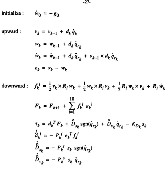
The key equations of the recursive algorithmn are given by the local inertial force of each link (3.23) and the spatial version of the adaptation law (3.28). Together with the definitions of the spatial quantities and some joint level computations for friction compensation and P.D. feedback, they form the complete algorithm.

initialize: _'0 = _{- go}

upward:

_{vk= k-l +}

_dk

_k

Wk = Wk-l

+

d

,rk

Wk = Wkl + dk rk + Vk-1 dk qk

ek = _k - Wk

downward:

f'

10

Fk Fk+1 + 1 fki aki

k =

dkFk

+ Dsk sgn('r

) + D

rk - KDk sk

fk

Ds

- Pk s

gn(rk)

Table 3-1: Complete Equations for the Recursive Implementation of the Direct Adaptive Controller

The algorithm consists of two major parts. During the first, the kinematic structure is traversed from the base upwards to the tip, while computing link velocities and accelerations. Then second part then proceeds in reverse order downwards from the tip to the base, at each link determining the individual forces, the joint torque, and updating the parameter estimates. Table 3-1 summarizes all involved equations for the case of diagonal gain matrices P and KD.

Several practical considerations can still greatly influence the actual efficiency of the algorithm :

* Using the Denavit-Hartenberg convention, the following choice of reference frames minimizes the number of frame transfonnations: velocities, accelerations, inertias, and local force components are expressed in their own frame (i.e. in the frame attached to their link), while joint-axes and summed fbrces are expressed with respect to the frame beneath them.

* It is important to "customize" the algorithm (similarly to e.g. [Koshla and Kanade, 1985]), so as to avoid multiplications by or additions with zero. These occur mainly in the local force component calculations (due to the sparse placement matrices), which should be evaluated analytically, as is described in Appendix B. Also, several velocity and acceleration components may be restricted to zero (especially close to the base) and can thus be eliminated.

* Several parameters may be redundant, and therefore the algorithm can be optimized by using a minimal parameter set, as is detailed in Chapter 4.

* The gravitational forces are implemented as a vertical acceleration in gravity-free space, by setting the spatial acceleration of the base appropriately.

3.8 Comparison to Newton-Euler and Walker Algorithm

The major difference between the true implementation algorithm developed above and both the Newton-Euler and [Walker, 1988] algorithm lies in the computation of the local force components. For comparison, the equivalent equations of all three algorithms are given by

ymp,

: (Y -g

) +

v x It w

+

w

x

I vt +

It wx

v

(3.29)

1

t ( l-g) + V x 11 v, (3.30)

-t

W

=

Quite cleariy, the deri.ved algorithmi for the actual implementation can be reduced to either algorithm, if reference hnd actual velocities are identical.

As a consequence of the above, a minor difference can also be found in the ad'.ptation segment of the [Walker, 1988] algorithm.

3.9 Closed K(inematic Chains

The above developments were detailed in the context of manipulators with open khilematic chains. They remain, however, also valid for manipulators with closed kinematic chains.

To implement the algorithm for closed chains, imaginary cuts are placed at several joints to obtain an open but branched kinematic structure. The forces are then simply added at the branch points and the constraint equations are used to determine the torques for the motorized joints. Notice that the link numbering system has to be changed and therefore also the ranges of the summations throughout the algorithm have to be modified. They must be specified as sets of links lying above or below, as is appropriate. The approach of [Walker, 1988] for structuring closed chains and incorporating kinematic constraints can be ,lsed straightforwardly.

Chapter 4

Minimal Parameterization

The inertial and mass properties of an arbitrary rigid body are completely described by 10 parameters, all of which are included in the spatial inertia matrix. They consist of the mass, the location of center of mass, and the six traditional inertia values. However, when two rigid bodies are connected through some joint and their motion is restricted with respect to each other, not all 20 parameters are needed to describe the behavior of the connected system. Consequently, the dynamics of a rigid manipulator can be described by a reduced set of inertial parameters ([An, Atkeson, and Hollerbach, 1985], [Khosla and Kanade, 1985]).

This parameter redundancy has been studied analytically by [Mayeda, 1988] for robots with rotational joints, whose axes are either perpendicular or parallel. He concludes the minimum number of parameters necessary to describe the whole system to be 7N-4B, where N is the number of links and B the number of parallel joints located at the base (which is at least one). If the first joint is vertical, then another two parameters can be

Parameter redundancy is quite important for both an efficient imhnplementation and the

estimation of the parameter values. The following therefore studies parameter reductions in

more detail, using the spatial notation to simplify the analysis. In particular, a system of

two consecutive links is examined and a procedure is derived, to eliminate redundant

parameters therein. Applying this procedure recursively to all connected links allows the

elimination of all redundant parameters of the manipulator and simultaneously gives rules

for the evaluation of the remaining parameters. The derivation is valid for arbitrary joint

types and configurations, including both rotational and translational joints of an arbitrary

intersection angles.

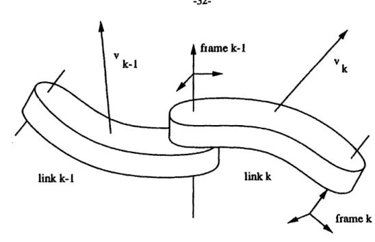
4.1 Parameter Redundancies for Two Consecutive Links

The following study focuses on two consecutive links k-1 and k connected by the particular joint, as is shown in Figure .4-1. The joint may be of any type and intersect other joint axes at any angle. The derived procedure allows a reduction of the original 20 inertial parameters, by transfering appropriate parameter values. That is, several parameter values can be set to zero, if other values are adjusted accordingly, without effecting the equations of motion.

In the following, the first link is assumed to have an arbitrary velocity and acceleration, that is it can move and turn in all directions. The case of restricted motions is a simple extension and is discussed later. The velocity of the secolld link can then determined using joint velocity and acceleration as

vk = Vk- 1 + dk ik (4.1)

k = Vk-1 + dkik + Vk-1 x dk 4k (4.2)

where d represents the joint axes, and v, i are the velocity and acceleration of the particular link.

V

k-I

link k-I

fimune k-I

link k

Figure

4-1:

Two

consecutive links connected by a rotational joint

To

assure that the parameter changes have no effect on the equations of motion two

conditions have

to

be satisfied. Given the velocities and accelerations both the total forces

and the joint torque must remain unchanged. That is, while changing the parameter values

the following must hold for any velocity and acceleration:

fk-I + fk = constant (4.3)

dkT

fk =

constant

(4.4)

where the individual link forces can be computed as

fk

= Ik k

_{k X I}

k

Vk

(4.5)

To evaluate these conditions the upper force fk can be rewritten as a function of the

lower link velocity and acceleration using Equations (4.1) and (4.2).

fk = Ik-I + _{vk- V X Ik}

Vk-1 (4.6)

+

Ik

dk qk

+ ( I

vk- X dk

dk

X

l

vkl

+

Vk-

+ dk lkdk qk2

To further study the parameter changes, an inertial variation matrix 81 is introduced. This matrix is added to the inertia matrix of link k and subtracted from that of link k-l, as the total inertia matrix must remain constant. Substituting in the above equations, equivalent conditions can be found for this inertia variation.

BI dk = 0 (4.7) 81 vk-l x dk + dk X 8, vk-l + Vk_ x .1 dk = 0 (4.8) dk X .I dk = 0 (4.9) dkT 81 ýk-l = 0 (4.10) dkT SI dk = 0 (4.11) dkT Vk- 1 x 81 vk- 1 = 0 (4.12)

However these conditions are redundant and in particular Conditions (4.9), (4.10), and (4.11) follow directly from Condition (4.7), while Equation (4.8) automatically implies Equation (4.12). That is, all inertia variations 51, which satisfy the following two conditions, describe parameter changes that have no effect on the equations of motion.

51 dk = 0 (4.13)

1 Vk-l1 dk + dk X 51 vk-1 + Vk- 1 x SI dk = 0 (4.14)

thus remain general for all joint types and configurations. To achieve further results a particular joint type has to be chosen, which specifies a value for the joint axis dk.

According to the Denavit-Hartenberg convention the joint axis is attached to frame k-1, so that the further analysis is best performed in this frame.

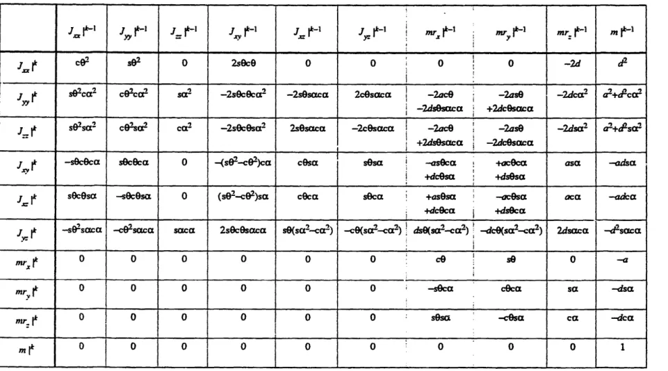
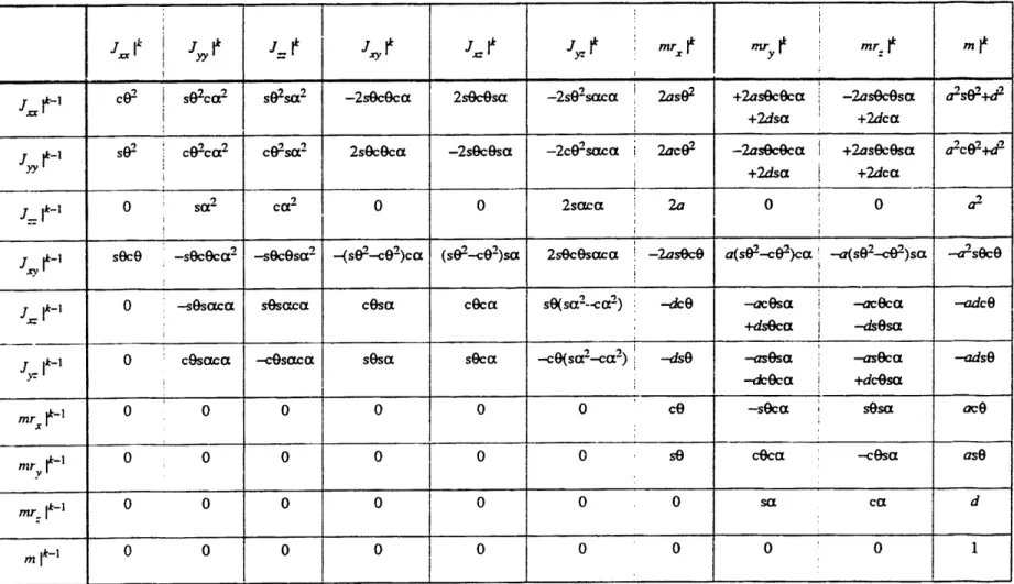
Evaluation of the above conditions can be done using Tables 4-1 and 4-2, which give the resulting spatial vector for unit values of vk- 1 and dk. Note the numbers enclosed in

brackets represent the values of the specified parameter, i.e. (3) is the value of parameter 3 (representing the z-axis inertia). They clearly show the dependence on the different inertia parameters. Given the value of dk, these tables then allow all necessary parameters and parameter combinations to be identified. The remaining parameters and parameter

combinations can therefore be included in the allowable set of inertia variations

61.

Using 81 it is now possible to eliminate parameters by subtracting their value from link k-1 and adding them to link k. This suggests the interpretation of transfering parameters from link k-I to link k, which can also be inverted, i.e. parameters can be transfered from link k to link k-l. To transfer the parameters, however, the inertia variations

61

was derived, to frame k. Tables 4-3 and 4-4 describe this transformation for both upward and downward directions.

dkl -(9) +(8) +(1) +(4) +(5) dk2 +(9)

-(7)

+(2)

+(6)

-(8)

+(3)

Table 4-1: Evaluation of

61 d

dk

dk

dk

-2(8)

-2(5)

dk

dk

sO2 0 2s"c 0 0 0 0 -2d

c 6' cOcr sc o -2socecca' -2sOsaca 2ceOsaca -2ac -2asOe -2dca2 '+ca'

-2dsesaE a +2dcfsaca

J se sa2 cOswa ca" -2sOcOsa 2 2sOsaca -2cOsaca -2acO -2asO -2dsa a2+d2sCZ

+2dsesaca -2dcOsacc

j*Y -sOceca sOcOca 0 -(se-cO2)ca c9sa sOsa -asOcca -+acca asa -ads&

i dcOsa +dsesa

=Ie sOcesa -secOscX 0 (se'-ceý)sa cOca seca +as0sa -acOsa aca -adca

+dcoca +dsOca

-se-saca --cessaca saca 2sOcOsaca sO(saQC caL ) -cO(saý2 ca2 dse(soa.caa ) -dcO(sca a ) 2dsaca -d-saca

0 0 0 0 0 0 cO

-- i 0 -- a

mr 0 0 0 0 0 0 -sOca cOca sa -dsa

r I 0 0 0 0 0 0 sesa -cOsa ca -dca

mk

0

0

0

0

0

4.2 Parameter Transfers through Rotational Joints

This section turns its attention to the particular case of rotational joints. However, the intersection angle between joint axes still remains arbitrary. Rotational joints are described by a unit rotation along the z-axis, so that

dk= 0

0

0

Therefore, assuming an unrestricted vk- 1 and using Tables 4-1 and 4-2, the equation

of motion depends on the following parameters and combinations.

(1)-(2) (3) (4) (5) (6) (7) (8) (4.16)

The inertia variation thus has three degrees of freedom and contains

1

k- =

(

(1) =(2) , (9) , (10) )

(4.17)

= ( =xxW= ) , Pz , 8m )

To eliminate and transfer parameters between links, the parameter values must undergo the reference frame transformation, given for rotational joint in Table 4-5. The Denavit-Hartenberg parameters (a,ct,d,O) correspond to joint k.

It is interesting to note that the parameter reductions often have physical interpretations. In this example the parameters correspond to a thin rod (i.e. having no inertia in that direction) along the rotational axis, which can belong to either of the attached links.

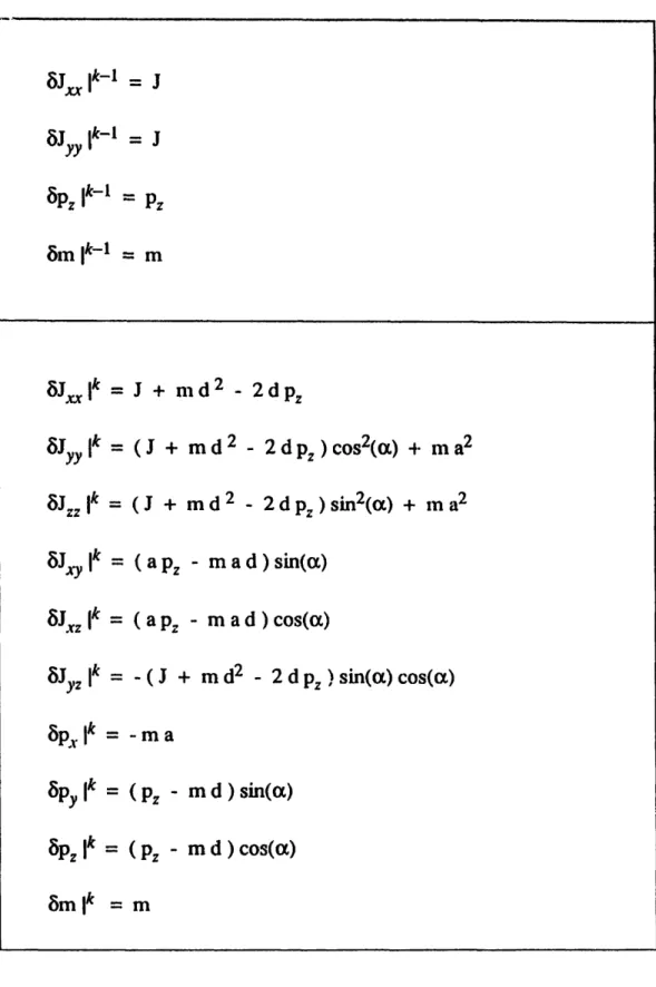
8Jxx Ik- I = J Jyy Ik-I = J 6pz Ik-I = Pz

6m

= (apz - mad )sin(a) = (apz - mad )cos(a)

= -(J + md 2 - 2dpz ) sin(a) cos(a)

=(Pz - md)sin(a)

pz Ik = (Pz - md ) cos(a)

Bm

Ik =m

Table 4-5: Transformation of the inertia parameters for rotational joints

8Jyy Ik

Jxyz Ik

8Jyr I

p.

Ik

-ma

4.3

Parameter Transfers through Translational Joints

Translational Therefore

dk =

joints are characterized by a unit translational vector along the z-axis.

(4.18)

As in the previous example using the Tables 4-1 and 4-2, the equation of motion depends on the following parameters and combinations.

(7) (8) (9) (10)

The inertia variation thus has six degrees of freedom and contains

61 ]k-1I _(4.20)

(1) ( ) ( 3), _{9 ' zz} J ( , _{y 'I} 6)_{xz I}

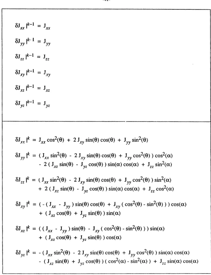
The reference frame transformation for these particular parameters is given in Table 4-6.

4.4

Parameter Reductions for Links with Restricted Motion

For links with restricted motion, as for example the base link, many more parameters can be eliminated. The analysis should proceed as before, however ignoring any conditions arising from the restricted directions. Also, only forces in the unrestricted directions need to be examined. As such situations only arise with very simple kinematics, the analysis is typically straight-forward. Foj exmnple, a base rotating about a vertical axis only requires the corresponding rotational inertia as parameters.

6Jx I_k- I _{= Jx}

5,jyy Ik

.1

8Jzz

-5Jx.r Ik = J cos2(0) + 2 Jxy sin(O) cos(6) + Jyy sin2(O)

8jy

- 2 ( Jxz sin() - Jyz cos(O) ) sin(ix) cos(ix) + Jzz sin2_(o)

FJzz Ik = (Jxx sin2_{(0) - 2 Jxy sin(0) cos(O) + Jy,, cos}2_{(0) ) sin}2_(x)

+ 2 ( Jxz sin(O) - Jyz cos(O) ) sin(cX) cos(Ox) + Jzz cos2_(Cx)

8Jxy

Ik

_{) )}

+ ( Jxz cos(0)

+

Jyr sin(0) ) sin(a)

Jxz Ik =( ( Jx - Jyy ) sin(0) - Jxy ( cs 2() - sin2(0) ) ) sin(a)

+ ( Jxz cos(6) + Jyz sin(O) ) cos("o)

Jyz Ik = - (J sin2() - 2 JAy sin(O) cos(0) + Jyy cos2(0) ) sin(ox) cos(Ix)

- ( Jx sin(O) + Jyz cos(0) ) ( cos 2() -sin2() ) + Jzz sin(ca) cos(oc)

Table 4-6: Transformation of the inertia parameters for translational joints

I

_ _ 'tt,

Chapter

5

Cartesian Implementation

The previous chapters analyzed the efficient implementation of a joint-space adaptive controller. Many tasks, however, are best described in terms of the end-effector motion or behavior. While it is possible to perform the inverse kinematics on a desired end-effector trajectory a-priori and thus to use a joint-space controller to achieve specified end-effector motions, such a procedure prevenws the implementation of an arbitrary end-effector behavior. Therefore, tasks that require interactions with the end-effector also necessitate a controller capable of utilizing cartesian data directly as t.a input (e.g., [Luh, Walker, and

Paul, 1980], [Khatib, 1980, 1983], in the non-adaptive case). This chapter discusses the problems of converting and extending the joint-space adaptive algorithms to handle cartesian data in real-time. The development represents a computational version of [Slotine

5.1 On-Line Inverse Kinematics

Taking a closer look at the joint-space controller, that is examing the control and adaptation laws (2.5) and (2.6), it can be interpreted as using only reference velocity and acceleration as input signals and guaranteeing convergence only to these. It is then the definition of the reference velocity in Equation (2.3) which guarantees the actual convergence to the desired trajectory. Since in the case of cartesian motion a desired joint trajectory is not given, it is possible to redefine the joint reference variables in tenns of its cartesian counterparts. More precisely, with cartesian reference velocity and acceleration defined as

x,. = d-AX - (5.1)

xr = Xd- A x (5.2)

where ~ = x - xd and A is again a s.p.d. matrix, the joint versions can be defined using the manipulator Jacobian J.

=,.

J q,.

(5.3)

x,.

-J ,. +

J

q,.

(5.4)

For non-redundant manipulators, the joint reference velocity and acceleration are then obtained by inverting the Jacobian.

q,.

=

~

_i.

_(5.5)

q,. = ,. - q)(5.6)

This simple extensron then provides a complete cartesian adaptive controller, which guarantees convergence of cartesian motion to the desired trajectory, similarly to the joint-space case, as long as singularities are avoided.

Note that the actual inverse kinematic solution for desired joint position is never computed directly but rather determined by the dynamics of the system. It can, however, be retrieved for other purposes by exploiting the filter structure of the reference velocity definition. Namely, implementing a filter of the form

Id + X

qd

X

will provide the exact desired joint trajectory. This also remains valid for redundant manipulators.

Also, to provide a more direct feedback or to achieve a certain behavior, it is also possible to add an explicit cartesian P.D. control component of the form

' = -JTKD (. -k,.) _(5.8)

Finally, note that many representations can be used for the end-effector orientation. For instance, defining the end-effector orientation as in [Luh, Walker, and Paul, 1980], with ( n ,

o

of ir be

xrorient

=

d+

(

nxnd

+

d

+

axad

)

(5.9)

guarantees that the orientation error and the angular velocity error both go to zero (with ; -;C. ). Following [Yuan, 19881, it is also possible to use Euler-parameters to represent the end-effector orientation, avoiding possible singularities of Euler-angles and rotations.

5.2 Redundancy Solution

For redundant manipulators the inverse Jacobian J-1, as was used above, is no longer uniquely defined. To resolve this non-uniqueness, a pseudo-inverse PJ can be used instead, which automatically minimizes the joint velocities corresponding to any cartesian velocities. In addition, the nullspace, i.e. the space of all joint motions which produce no cartesian motion, can be used to minimize any performance index.

Similar to work done by [Klein and Huang, 1983], [Klein and Blaho, 1987], the performance index is chosen to be a quadratic norm of joint positions. Such an approach is computationally efficient and, intuitively, mimics r. "flexible beam" clamped to the desired endpoint trajectory. It thus helps to keep the manipulator away from joint limits, as well as from singular positions. In addition, cyclic cartesian motions converge to cyclic joint motions [see also Baker and Wampler, 1988], avoiding joint trajectory drifts associated with mere pseudo-inverse methods.

In contrast to other controllers, sliding controllers require both reference velocity and acceleration, so that besides the pseudo-inverse (or generalized inverse) J+ of the Jacobian

J, its time-derivative is also needed. Assuming a Jacobian of linearly independent rows,

that is a Jacobian describing a redundant manipulator outside of singularities, we can write explicit expressions for both as

J+ = JT ( JT)-I (5.10)

+ = -J+jJ+ + (1-J+J)jT(Jjf)- 1 (5.11)

With these results the inverse kinematic transformnnation for a redundant manipulator can be specified as