HAL Id: hal-02417275
https://hal.umontpellier.fr/hal-02417275
Submitted on 18 Dec 2019
HAL is a multi-disciplinary open access
archive for the deposit and dissemination of
sci-entific research documents, whether they are
pub-lished or not. The documents may come from
teaching and research institutions in France or
abroad, or from public or private research centers.
L’archive ouverte pluridisciplinaire HAL, est
destinée au dépôt et à la diffusion de documents
scientifiques de niveau recherche, publiés ou non,
émanant des établissements d’enseignement et de
recherche français ou étrangers, des laboratoires
publics ou privés.
Generation of Binary Tree-Child phylogenetic networks
Gabriel Cardona, Joan Carles Pons, Celine Scornavacca
To cite this version:
Gabriel Cardona, Joan Carles Pons, Celine Scornavacca. Generation of Binary Tree-Child phylogenetic
networks. PLoS Computational Biology, Public Library of Science, 2019, 15 (10), pp.e1007440.
�hal-02417275�
Generation of Binary Tree-Child phylogenetic networks
Gabriel Cardona1*, Joan Carles Pons1, Celine Scornavacca2
1Department of Mathematics and Computer Science, University of the Balearic Islands, Ctra. de Valldemossa, km. 7.5, E-07122 Palma, Spain
2Institut des Sciences de l’Evolution (ISE-M), Universit´e de Montpellier, CNRS, IRD, EPHE, 34095 Montpellier Cedex 5, France
Abstract
Phylogenetic networks generalize phylogenetic trees by allowing the modelization of events of reticulate evolution. Among the different kinds of phylogenetic networks that have been proposed in the literature, the subclass of binary tree-child networks is one of the most studied ones. However, very little is known about the combinatorial structure of these networks.
In this paper we address the problem of generating all possible binary tree-child (BTC) networks with a given number of leaves in an efficient way via
reduction/augmentation operations that extend and generalize analogous operations for phylogenetic trees, and are biologically relevant. Since our solution is recursive, this also provides us with a recurrence relation giving an upper bound on the number of such networks.
We also show how the operations introduced in this paper can be employed to extend the evolutive history of a set of sequences, represented by a BTC network, to include a new sequence.
An implementation in python of the algorithms described in this paper, along with some computational experiments, can be downloaded from
https://github.com/bielcardona/TCGenerators.
Author summary
Phylogenetic networks are widely used to represent evolutionary scenarios with reticulated events, and among them, the class of binary tree-child (BTC for short) networks is one of the most studied ones. Despite its importance, BTC networks, as mathematical objects, are not yet fully understood. In this paper we introduce two operations (reduction and augmentation) on the set of BTC networks that generalize well known operations on phylogenetic trees, and show how they can be used to analyze and synthesize any BTC network. Apart from the mathematical formulation of the problem, we exhibit how these operations can be used in biological applications to add a new sequence to a given BTC network. This can be useful, for instance, to update the network without redoing the whole search, or in a phylogenetic placement perspective. We also obtain a recursive formula for a bound on the number of such networks. We have implemented the algorithms in this paper, made them available on a public repository, and used this implementation to perform some computational simulations.
Introduction
Phylogenetic networks are, mathematically, a generalization of phylogenetic trees that, containing nodes with more than one ancestor, permit to model reticulated evolutionary events such as recombinations, lateral gene transfers and hybridizations.1
In this paper, we shall focus on directed phylogenetic networks (see [3] for a short survey on the phylogenetic network paradigm also covering undirected phylogenetic networks). Mathematically, such networks are, in the broadest sense, directed acyclic graphs with a single node with no incoming arcs –the root– representing the common ancestor of all the Operational Taxonomic Units (OTUs for short) under study, which are represented by the nodes with no outgoing arcs –the leaves– of the graph; internal nodes represent either (hypothetical) speciations or (hypothetical) reticulated events. Nodes with a single incoming arc –tree nodes– model extant or non-extant OTUs, and arcs between tree nodes model direct descent through mutation; nodes with two incoming arcs –hybrid nodes– model reticulated events involving the OTUs
corresponding to the two parents of the node under consideration, and whose resulting OTU is modeled as its single child. Unfortunately, this definition is too broad, both for representing biologically-meaningful evolutionary scenarios, and for giving objects that can be efficiently handled.
So far, several restrictions on this general definition have been introduced in the literature. A few of them are based on biological considerations, while the majority have been introduced to artificially narrow the space of networks under study. This led to the introduction of a panoply of different classes of phylogenetic networks, such as
time-consistent networks [4], regular networks [5], orchard networks [6], galled trees [7] and galled networks [8], level-k networks [9], tree-sibling networks [10], tree-based networks [11] and LGT networks [12], just to name a few.
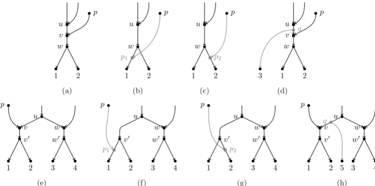
In this paper, we shall focus on binary tree-child networks (BTC networks, for short), which were introduced by [10] and are one of the most studied classes of phylogenetic networks [13–16]. Mathematically, being tree-child means that every internal node is compelled to have at least a child node that is a tree node. BTC networks have been introduced in order to adjust a complex biological reality in a computationally tractable way. Although the original motivation for these networks is not biological, and hence they present some limitations, the mathematical constraint on BTC networks translates biologically as follows: every non-extant OTU is required to have at least an offspring species that evolved only through mutation. This means that not all biologically-meaningful evolutionary scenarios can be modeled with BTC networks. For example, the scenarios depicted in Fig 1(a,e) are not allowed since, in these cases, the node labeled with u has no child with a single incoming arc. Still, BTC networks are one of the most permissive classes of phylogenetic networks and they permit to model quite a lot of meaningful scenarios, and those that cannot be modeled can be approximated pretty well, see Fig 1.
The combinatorial study of phylogenetic networks is nowadays a challenging and active field of research. Nevertheless, the problem of counting how many phylogenetic networks are in a given subclass of networks is still open even for long-established classes. More precisely, this problem has been only recently solved for galled
networks [18]; for other classes, including tree-child networks, we only have asymptotic results [19, 20]. Associated to the problem of counting networks, we find the problem of their “injective” generation, i.e. without having to check for isomorphism between pairs of constructed networks.
1We note here that other representations, for example gene tree-species tree reconciliations [2],
permit to model scenarios including other classes of evolutionary events such as duplications, losses and transfers of genes.
p u v w 1 2 (a) p u w 1 2 p1 (b) p u w 1 2 p2 (c) p u v w 1 2 q 3 (d) 1 2 3 4 v0 w0 v w u p (e) 1 2 3 4 v0 w0 w u p p1 (f) 1 2 3 4 v0 w0 w u p p2 (g) 1 2 3 4 v0 w0 v w u p 5 q (h) Fig 1. Limitations of BTC networks. The scenarios in (a) and (e) are not BTC networks since in both cases the node labeled with u has no tree-node child. Still, the scenario in (a) can be approximated either by the scenario in (b) or by that in (c), both scenarios being BTC networks. Also, if we are lucky enough to find an OTU between the hybrid event represented by the node u and that represented by v, e.g. the node q in (d), then the hybrid event in v can be modeled. The same reasoning holds for the scenario in (e) and those in (f,g,h). Thus, if the “true” network is not BTC, we can always find a BTC network those topology is not far from the true one. In our example, the networks in (b,c) are both a head-moving rSPR [1] away from the true network in (a). The same holds for the networks in (f,g) w.r.t. the one in (e). In general, each
violation of the TC property, i.e. each hybrid node that has only hybrid children, moves the reconstructible network a head-moving rSPR away from the true one. Note that the configuration in (a) is known to generate severe indistinguishability issues [17].
The main result of this paper is a systematic way of recursively generating, with unicity, all BTC networks with a given number of leaves. This generation relies on a pair of reduction/augmentation operations –both producing BTC networks– where reductions decrease by one the number of leaves in a network, and augmentations increase it. The idea of using pairs of operations has already been used to deal either with other classes of phylogenetic networks [21, 22], or for BTC networks but without the unicity feature [6].
In order to give a biological meaning to these augmentation operations, assume that the evolutive history of a given group of species is known and modeled by a BTC network, and a new species has to be taken into account. The augmentation operation determines exactly how the phylogenetic network has to be modified, and what is the minimum information needed to establish this modification, in order to model the evolution of the group of species with the newly incorporated one.
As an interesting side product, this procedure gives a recursive formula providing an upper bound on the number of BTC networks. Note also that being able to generate all BTC networks with a given number of leaves may also be interesting as part of a divide-and-conquer framework to reconstruct phylogenetic networks, where we start by computing BTC networks on 3/5 leaves that are then combined together, as done for example in [23, 24].
The paper is organized as follows. In Section Methods, we review the basic definitions that will be used throughout the paper. The main part of the paper is in Section Results, which is split between different subsections. Subsection Reduction of
Networks is devoted to the reduction procedure, while in Subsection Generation of Networks we introduce the augmentation operation and prove that any BTC network can be obtained, in a unique way, via a sequence of augmentation operations applied to the trivial network with one leaf. In Subsection Bounding the Number of Networks, we show how to relax the conditions for the applicability of the augmentation operation to obtain a recursive formula providing an upper bound on the number of BTC networks. In Subsection An Application to Phylogenetic Reconstruction, we give a concrete biological application of the methods we have developed. In Subsection Computational Experiments, we introduce the implementation of the algorithms presented in the paper, and some experimental results, including the exhaustive generation of all BTC networks with up to six leaves and an upper bound of their number up to ten leaves. Finally, in Section Conclusion we discuss how our reduction/augmentation operations extend and generalize analogous operations for phylogenetic trees.
Methods
In this section we introduce the mathematical notations that are used in the rest of the paper.
Throughout this paper, a tree node in a directed graph is a node u whose pair of degrees d(u) = (indegree u, outdegree u) is (1, 0) for the leaves, (0, 2) for the roots, or (1, 2) for internal tree nodes; a hybrid node is a node u with d(u) = (2, 1). If two nodes
u and v are linked by an arc (u, v) we say that u is a parent of v, or that v is a child of u. Also, two nodes are siblings if they have a common parent.
A binary phylogenetic network over a set X of taxa is a directed acyclic graph with a single root such that all its nodes are either tree nodes or hybrid nodes, and whose leaf set is bijectively labeled by the set X. In the following, we will implicitly identify every leaf with its label. A binary phylogenetic network is tree-child if every node either is a leaf or has at least one child that is a tree node [10]; in particular, the single child of a hybrid node must be a tree node. We will denote byBT Cn the set of binary tree-child
phylogenetic networks over the set [n] ={1, . . . , n}.
An elementary node in a directed graph is a node u with d(u) = (1, 1) or
d(u) = (0, 1). An elementary path p is a path u1, . . . , uk composed of elementary nodes
such that neither the single parent of u1(if it exists) nor the single child of uk are
elementary. We call these last two nodes respectively the grantor (if this node is well-defined) and heir of the nodes in the elementary path. In case of an elementary node, its grantor and heir are those of the nodes in the single elementary path that contains the given node. The elimination of an elementary path p consists in deleting all nodes in p, together with their incident arcs, and adding an arc between the grantor and the heir of p (provided that the grantor exists; otherwise, no arc is added). The elimination of an elementary node is defined as the elimination of the elementary path that contains the given node.
Given a node u, we can split it by adding a new node ˜u, an arc (˜u, u), and replacing every arc (v, u) with (v, ˜u). If u is a tree node, then ˜u is an elementary node whose heir is u, and the elimination of ˜u recovers the original network. The successive splitting (say k times) of a tree node u generates an elementary path formed by k nodes, whose
heir is u, and whose elimination recovers the original network. Fig 2 illustrates the definitions given in this section.
1 2 3 4 x y v w u e1 e2
Fig 2. The definitions introduced in the Methods Section. For the network N in the figure (black nodes and arcs only), we have the following: X ={1, 2, 3, 4} is the set of taxa, u is the root, x is a hybrid node and all other nodes are internal tree nodes. If we split v twice by adding the elementary nodes e1 and e2 in grey, we have that
(e1, e2) is an elementary path with grantor and heir equal respectively to u and v. N is
a binary tree-child network since both parents v and w of the only hybrid node x have another child (1 and y, respectively) that is a tree node.
Results
Reduction of Networks
The goal of this subsection is to define a reduction procedure on BTC networks that can be applied to any such network, and producing a BTC network with one leaf less. By successive application of this procedure, any BTC network can thus be reduced to the trivial network with a single leaf.
We start by associating to each leaf ` a path whose removal will produce the desired reduction (up to elementary paths).
Let ` be a leaf of a BTC network N . A pre-TH-path for ` is a path u1, . . . , ur= `
such that (see Fig 3):
1. Each node ui in the path is a tree node.
2. For each i = 1, . . . , r− 1, the child of ui different from ui+1, denoted by vi, is a
hybrid node.
3. For each i6= j, we have that vi6= vj.
u1 ui ur−1 ur= ` v1 vi vr−1 .. . .. .
Fig 3. A pre-TH-path for the leaf`. Tree nodes are represented by circles and hybrid nodes by squares; snake arrows represent paths. The path inside the dotted box is a pre-TH-path for `.
A TH-path is a maximal pre-TH-path, i.e. a pre-TH-path that cannot be further extended. Note that, since all nodes in a pre-TH-path p are tree nodes, if p can be extended by prepending one node, then this extension is unique. Hence, starting with the trivial pre-TH-path formed by the leaf ` alone, and extending it by prepending the parent of the first node in the path as many times as possible, we obtain a TH-path that is unique by construction. Let u1, . . . , ur= ` be a TH-path; different possibilities
may arise that make it maximal: (1) u1 is the root of N ; (2) the parent of u1, call it x,
is a hybrid node; (3) x is a tree node whose both children are tree nodes; (4) x is a parent of vi for some i∈ [r − 1]. We shall see in Lemma 1 that the first case cannot
hold; the other three possibilities are depicted in Fig 4.
u1 ui ur−1 ur= ` v1 vi vr−1 .. . .. . x u1 ui ur−1 ur= ` v1 vi vr−1 .. . .. . x u1 ui ur−1 ur= ` v1 vi vr−1 x .. . .. .
Fig 4. The different possibilities for the TH-path of a leaf `. Depiction of the conditions (2), (3) and (4), respectively, under which a pre-TH-path cannot be extended, making the path inside the dotted box a TH-path for `.
For each leaf `, we denote by TH(`) its single TH-path and by TH(`)1the first node
of this path. Note that we allow the case r = 1. In this case, if we are not in a trivial BTC network (i.e. a network consisting of a single node), the parent of ` is either a hybrid node, or a tree node whose two children are tree nodes.
Lemma 1. Let N be a non-trivial BTC network and let ` be any of its leaves. Then, TH(`)1 cannot be the root of N .
Proof. Let u1, . . . , ur= ` be the path TH(`) and assume for the sake of contradiction
that u1 is the root of N . For each i = 1, . . . , r− 1, let vi be the hybrid node that is a
child of ui and xi the parent of vi different from ui (see Fig 5); recall that xi does not
belong to TH(`) by the definition of a pre-TH-path. Since u1is the root of N , every
node of N either belongs to the path TH(`) or is descendant of a node in
{vi| i ∈ [r − 1]}. In particular, for each i ∈ [r − 1], there exists some σ(i) ∈ [r − 1] such
that xi is descendant of vσ(i), and since this node is descendant of xσ(i), xi is
descendant of xσ(i). Hence, starting with x1we get a sequence x1, xσ(1), xσ(σ(1)), . . .
where each node in the sequence is a descendant of the following one. Since there is a finite number of nodes, at some point we find a repeated node, which means that N contains a cycle and hence we have a contradiction.
We say that a leaf ` is of type T (resp. of type H) if the parent of TH(`)1is a tree
node (resp. a hybrid node). If ` is of type H, we indicate by TH(`) the path obtained by prepending to TH(`) the parent of TH(`)1. For convenience, we let TH(`) = TH(`)
u1 uσ(i) ui ur−1 ur= ` vi vσ(i) xσ(i) xi .. . .. . .. .
Fig 5. The first node in a TH-path cannot be the root. Illustration of the nodes involved in the proof of Lemma 1.
Definition 1. Let ` be a leaf in a BTC network N . We define the reduction of N with respect to ` as the result of the following procedure (see Figs 6 and 7):
1. Delete all nodes in TH(`) (together with any arc incident on them). 2. Eliminate all elementary nodes.
We indicate this reduction by R(N, `). If we want to emphasize the type of the deleted leaf, we indicate the reduction by T (N, `) and say it is a T -reduction if ` is of type T , or by H(N, `) and say that it is a H-reduction if ` is of type H.
w1 u0= u1 ui ur−1 ur= ` v1 vi vr−1 x1 y1 xi yi xr−1 yr−1 t1 z1 .. . .. . x1 y1 xi yi xr−1 yr−1 .. . .. . t1 z1
Fig 6. Reduction operation of typeT . Depiction of the reduction operation T (N, `). The nodes inside the dotted box form TH(`) and will be removed, which will create elementary nodes that will be substituted by arcs.
To ease of reading, we shall introduce some notations that will be used hereafter and are also illustrated in Figs 6 and 7:
Definition 2. Let u1, . . . , ur= ` be the path TH(`) and let u0 be the first node in
TH(`). For each i∈ [r − 1], vi is the hybrid child of ui, xithe parent of vidifferent from
u0 u1 ui ur−1 ur= ` v1 vi vr−1 x1 y1 xi yi xr−1 yr−1 w2 w1 z1 t1 z2 t2 .. . .. . x1 y1 xi yi xr−1 yr−1 z1 t1 z2 t2 .. . .. .
Fig 7. Reduction operation of typeH. Depiction of the reduction operation H(N, `). The nodes inside the dotted box form TH(`) and will be removed, which will create elementary nodes that will be substituted by arcs.
always a tree node, zj is its parent (if it exists, since wj could be the root of N ), and tj
its child different from u0, where j = 1 for T -reductions and j∈ [2] for H-reductions.
Remark 1. Since N is tree-child, the nodes yi are always tree nodes, and so are t1and
t2 in case of an H-reduction. In case of a T -reduction, by definition of a TH-path, t1 is
either a tree node or coincides with one of the hybrid nodes vi. Also, the removal of the
arcs of the form (ui, vi) and (wj, u0) makes nodes vi and wj elementary in N\ TH(`),
where i∈ [r − 1], and j = 1 for T -reductions and j ∈ [2] for H-reductions. Since no other arc is removed, no other node can be elementary. In order to find the heirs of nodes vi and wj, we must analyse under which circumstances two of these elementary
nodes are adjacent in N\ TH(`).
1. If we had that two nodes vi and vj were connected by an arc in N\ TH(`), then
the single child of a hybrid node in N would be also a hybrid. This contradicts the fact that N is tree-child.
2. The existence of an arc (vi, wj) would imply the existence of a cycle in N , which
is impossible.
3. Consider now the case of an arc (wj, vi). In case of an H-reduction, it would
imply that both children of wj are hybrid nodes, which is impossible. However,
such an arc can be present in a T -reduction: when t1 is equal to vi. In this last
case, w1 and vi form an elementary path in N\ TH(`) and their common heir is
yi (see Fig 8).
4. Finally, in case of an H-reduction, it can exist an arc between w1 and w2, say that
the arc is (w1, w2) (which implies, t1= w2, z2= w1). In this case, w1 and w2
form an elementary path in N\ TH(`) and their common heir is t2(see Fig 9).
In all other cases, the elementary nodes vi and wj are isolated, and their respective
heirs are yi and tj.
We study now what we call the recovering data of a reduction. This information will be used in the next subsection to recover the original network from its reduction.
w1 u0= u1 ui ur−1 ur= ` v1 vi= t1 vr−1 y1 yi yr−1 z1 .. . .. . y1 yi z1 yr−1 .. . .. .
Fig 8. Reduction operation of typeT (particular case). Particular case of the reduction operation of type T when t1= vi for some i∈ [r − 1].
u0 u1 ui ur−1 ur= ` v1 vi vr−1 y1 yi yr−1 w2= t1 z2= w1 t2 z1 .. . .. . y1 yi yr−1 z1 t2 .. . .. .
Fig 9. Reduction operation of typeH (particular case). Particular case of the reduction operation of type H when w1 and w2are linked by an arc.
Definition 3. The recovering data of the reduction N0= R(N, `) is the pair (S 1, S2),
where:
• S1is the multiset of the nodes of N0 that are heirs of the nodes wj. The
cardinality of S1 (as a multiset) is either 1 or 2, depending on the type of the
reduction, and will be denoted by |S1|.
• S2is the tuple (y1, . . . , yr−1) of nodes of N0, which are the heirs of the nodes vi.
This tuple could be empty, corresponding to the case r = 1.
We introduce now a set of conditions on multisets and tuples of nodes, and prove that the recovering data associated to any of the defined reductions satisfies them. Definition 4. Given a BTC network N0 and a pair (S
1, S2) with
• S1a multiset of tree nodes of N0,
• S2= (y1, . . . , yr−1), with r≥ 1, a (potentially empty) tuple of r − 1 tree nodes of
consider the following set of conditions:
1. For every i, j ∈ [r − 1] with i 6= j, the nodes yi and yj are different, and if they
are siblings, then yi∈ S1or yj∈ S1.
2. For every i∈ [r − 1], if yi is the child of a hybrid node or has a hybrid sibling,
then yi∈ S1.
3. No node in S1is a proper descendant of any node in S2.
4T. |S1| = 1.
4H. |S2| = 2 and no node of S1 appears in S2.
We say that (S1, S2) is T -feasible if it satisfies conditions 1, 2, 3, and 4T, and H-feasible
if it satisfies conditions 1, 2, 3, and 4H. Finally, we say that (S1, S2) is feasible if it is
either T -feasible or H-feasible.
Proposition 2. Let N0 = T (N, `) be a T -reduction of a BTC network N . Then, its
recovering data({τ1}, (y1, . . . , yr−1)) is T -feasible.
Proof. First, note that, by Remark 1, all nodes in ({τ1}, (y1, . . . , yr−1)) are tree nodes
and that Condition 4T holds trivially. Note also that τ1 is equal to yi if t1= vi, or to t1
if this node is different from all the nodes vi. We now prove that Conditions 1, 2 and 3
hold:
1. If yi= yj, then in N we have vi= vj, which is impossible by definition of
TH-path. If yi and yj are siblings in N0 but none of these nodes is equal to τ1,
then vi and vj are siblings in N , which implies that their common parent has two
hybrid children, which is impossible in a BTC network.
2. If yi is the child in N0 of a hybrid node and τ16= yi, then in N we have that vi,
which is a hybrid node, is the child of a hybrid node, which is impossible in a tree-child network. Analogously, if yi has a sibling in N0 which is a hybrid node,
and yi 6= τ1, then in N we have that vi is sibling of another hybrid node, which is
again impossible.
3. The existence of a non-trivial path in N0 from y
i to τ1 would, by construction,
imply the existence of a path from yi to w1in N . Since there exists also a path in
N from w1 to yi, this would contradict the fact that N is a DAG.
Proposition 3. Let N0 = H(N, `) be an H-reduction of a BTC network N . Then, its
recovering data({τ1, τ2}, (y1, . . . , yr−1)) is H-feasible.
Proof. Again we have, by Remark 1, that all nodes in the recovering data are tree nodes. Additionally, by the same remark, we have that|S1| = 2 –and hence the first
part of Condition 4H holds– and if (w1, w2) is an arc of N , then S1={t2, t2}, otherwise
S1={t1, t2} with t16= t2. Note that Condition 3 implies that Conditions 1 and 2 can
be simplified as follows: for all i, j∈ [r − 1] with i 6= j, yi and yj are neither equal nor
siblings, and for all i∈ [r − 1], yi is neither the child nor the sibling of a hybrid node.
Conditions 1 and Conditions 2 and 3 in their simplified form follow using the same arguments as in the previous proposition. As for the condition 4H, the nodes τ1 and τ2
are different from the nodes yi since the parents of τ1 and τ2 in N are tree nodes, while
The following proposition is the main result of this subsection, since it shows that the reduction that we have defined, when applied to a BTC network, gives another BTC network with one leaf less. Hence, successive applications of these reductions reduce any BTC network to the trivial BTC network.
Proposition 4. Let N be a BTC network over X and ` one of its leaves. Then, R(N, `) is a BTC network over X\ {`}.
Proof. First, it is easy to see that, since no new path is added, the resulting directed graph is still acyclic.
Then, we need to check that R(N, `) is binary. To do so, we start noting that every node in N\ TH(`) is either a tree node, a hybrid node, or an elementary node. Indeed, the removal of TH(`) (Phase 1 of Definition 1) only affects the nodes adjacent to this path, that is the nodes vi and wi, which, as shown in Remark 1, become elementary.
The elimination of all elementary nodes (Phase 2 of Definition 1) does not affect the indegree and outdegree of any other node, apart when the root ρ of N\ TH(`) is elementary. In such a case, the heir of ρ becomes the new root. Hence, R(N, `) is binary and rooted.
Note also that the set of leaves of R(N, `) is X\ {`}, since in N \ TH(`) no node becomes a leaf and the only leaf that is removed is `.
Finally, we need to prove that R(N, `) is tree-child. Note that, from what we have just said about how the reduction affects indegrees and outdegrees of the nodes that persist in the network, it follows that each hybrid node of R(N, `) is also a hybrid node of N , and that its parents in R(N, `) are the same as in N . It follows that no node in R(N, `) can have that all its children are hybrid, since this would imply that N is not tree-child, a contradiction.
Corollary 5. LetN ∈ BT Cn be a BTC network over[n]. Let Nn= N and define
recursively Ni= R(Ni+1, i + 1) for each i = n− 1, n − 2, . . . , 1. Then, Ni is a BTC
network over[i]. In particular, N1 is the trivial BTC network with its single node
labeled by 1.
We finish this subsection with the computation of the number of tree nodes and hybrid nodes that the reduced network has, both in terms of the original network and of the reduction operation that has been applied. But before, we give an absolute bound on the number of these nodes in terms of the number of leaves.
Lemma 6. Let N be BTC network over [n] with t tree nodes and h hybrid nodes. Then t− h = 2n − 1, h ≤ n − 1 and t ≤ 3n − 2.
Proof. The equality t− h = 2n − 1 follows easily from the handshake lemma taking into account the number of roots, internal tree nodes, leaves and hybrid nodes in N , and their respective indegrees and outdegrees. The inequality h≤ n − 1 is shown in Proposition 1 in [10], and the last inequality is a simple consequence of the equality and the inequality already proved.
Proposition 7. Let N be a BTC network and ` one of its leaves, and N0= R(N, `). Let t, h (resp. t0, h0) be the number of tree nodes and hybrid nodes ofN (resp. of N0). Then
t0= t− |TH(`)| − 1, h0 = h− |TH(`)| + 1, where|TH(`)| is the number of nodes in TH(`).
Proof. Since the number of tree nodes and hybrid nodes are linked by the equality in Lemma 6, it is enough to prove that h0= h− |TH(`)| + 1. From the discussion in Remark 1, it is straightforward to see that the number of hybrid nodes in N that are not in N0 is r− 1 if ` is of kind T , and r otherwise. Hence, in both cases we have h0= h− (|TH(`)| − 1) and the result follows.
Generation of Networks
In this subsection, we consider the problem of how to revert the reductions defined in the previous subsection, taking as input the reduced network and its recovering data. This will allow us to define a procedure that, starting with the trivial BTC network with one leaf, generates all the BTC networks with any number of leaves in a unique way.
We start by defining two augmentation procedures that take as input a BTC network and a feasible pair, and produce a BTC network with one leaf more. Definition 5. Let N be a BTC network over X, ` a label not in X, and
({τ1}, (y1, . . . , yr−1)) a T -feasible pair. We apply the following operations to N (see
Fig 10):
1. Create a path of new nodes u1, . . . , ur.
2. Split the node τ1 creating one elementary node w1 and add an arc (w1, u1).
3. For each node yi, split it introducing one elementary node viand add an arc
(ui, vi).
4. Label the node ur by `.
We denote by T−1(N, `;{τ
1}, (y1, . . . , yr−1)) the resulting network and say that it has
been obtained by an augmentation operation of type T .
y1 yi yr−1 .. . .. . τ1 w1 u1 ui ur−1 ur= ` v1 vi vr−1 y1 yi yr−1 τ1 .. . .. .
Fig 10. Augmentation operation of type T . Depiction of the augmentation operation T−1(N, `;{τ
1}, (y1, . . . , yr−1)) when τ16= yi for all i∈ [r − 1].
Note that the order in which steps 2 and 3 are done is relevant in the case that τ1= yi for some i∈ [r − 1]. In such a case, two nodes w1and vi are created, linked by
an arc (w1, vi) (see Fig 11).
Proposition 8. Using the notations of Definition 5, the network ˜
N = T−1(N, `;{τ1}, (y1, . . . , yr−1))
is a BTC network over X∪ {`}. Moreover, if N has h hybrid nodes, then ˜N has h + r− 1 hybrid nodes.
Proof. We first check that the resulting directed graph is acyclic. Let us assume that ˜N contains a cycle. If we define U1={u1, . . . , ur} and U2= V ( ˜N )\ U1, we have that the
y1 yi= τ1 yr−1 .. . .. . w1 u1 ui ur−1 ur= ` v1 vi vr−1 y1 yi yr−1 .. . .. .
Fig 11. Augmentation operation of type T (particular case). Depiction of the augmentation operation T−1(N, `;{τ
1}, (y1, . . . , yr−1)) when τ1= yi.
only arc connecting U2with U1. The cycle can be contained neither inside U1, since
these nodes are linked by a single path, nor inside U2, since otherwise N would contain
a cycle. Hence, the cycle must contain at least the arc (w1, u1) and an arc (ui, vi). This
implies the existence of a path from vi to w1 visiting only nodes in U2, which in turn
means that N contains a path from yi to τ1, against Condition 3 of Definition 4.
Note that the nodes in U1 are tree nodes by construction. Also by construction, the
node w1is a tree node, the nodes vi are hybrid nodes and ur is a leaf which is labelled
with `. Finally, the other nodes keep the same degrees they had in N and hence ˜N is a binary phylogenetic network over X∪ {`} with h + r − 1 hybrid nodes.
Since N is tree-child, in order to check that ˜N is also tree-child, we only need to check the newly added hybrid nodes, which are the parents of the nodes vi.
Let us first consider the case that τ16= yi for all i∈ [r − 1]. For each node vi, its
parents are ui and the parent xi of yi in N . The node ui is by construction a tree node
whose other child is ui+1, which, in turn, is a tree node. Since τ16= yi, by Condition 2
of Definition 4, yi can have neither a hybrid parent nor a hybrid sibling, and it cannot
be a sibling of any other node yj with j∈ [r − 1]. This latter restriction implies that yi
has the same sibling ˜xiin N and ˜N . Thus both xi and ˜xi are not hybrid nodes, and the
network is tree-child.
Let us now consider the case that τ1= yi for a single choice of i∈ [r − 1]. The
hybrid node vi in ˜N has as parents the nodes w1 and ui, and these two nodes have as
respective children u1and ui+1, which are tree nodes. For each other node vj with j6= i
and such that yj is a not sibling of yi, the same argument as in the previous case proves
that both parents of vj have a tree child. If yj is a sibling of yi, it is easy to see that the
parent of vj is still tree-child since it has w1as child.
Definition 6. Let N be a BTC network over X, ` a label not in X, and
({τ1, τ2}, (y1, . . . , yr−1) a H-feasible pair. We apply the following operations to N (see
Fig 12):
1. Create a path of new nodes u0, u1, . . . , ur.
2. Split each of the nodes τi introducing one elementary node wi and add an arc
from wi to u0. Note that, if τ1= τ2, two consecutive elementary nodes must be
created (see Fig 13 for this case).
3. For each node yi, split it introducing one elementary node viand add an arc
4. Label the node ur by `.
We denote by H−1(N, `;{τ
1, τ2}, (y1, . . . , yr−1)) the resulting network and say that it
has been obtained by an augmentation operation of type H.
y1 yi yr−1 τ1 τ2 .. . .. . u0 u1 ui ur−1 ur= ` v1 vi vr−1 y1 yi yr−1 w2 w1 τ1 τ2 .. . .. .
Fig 12. Augmentation operation of type H. Depiction of the augmentation operation H−1(N, `;{τ1, τ2}, (y1, . . . , yr−1)) when τ16= τ2. y1 yi yr−1 τ1= τ2 .. . .. . u0 u1 ui ur−1 ur= ` v1 vi vr−1 y1 yi yr−1 w2 w1 τ1= τ2 .. . .. .
Fig 13. Augmentation operation of type H (particular case). Depiction of the augmentation operation H−1(N, `;{τ
1, τ2}, (y1, . . . , yr−1)) when τ1= τ2.
Proposition 9. Using the notations of Definition 6, the network ˜
N = H−1(N, `;{τ1, τ2}, (y1, . . . , yr−1))
is a BTC network over X∪ {`}. If N has h hybrid nodes, then ˜N has h + r hybrid nodes.
Proof. The proof is completely analogous to that of Proposition 8, taking into account that one extra hybrid node is created.
Given a BTC network over X, a label ` /∈ X and a feasible pair (S1, S2), in order to
unify notations we define the augmented network R−1(N, `; S
1, S2) as T−1(N, `; S1, S2),
if|S1| = 1, and as H−1(N, `; S1, S2), if|S1| = 2. Also, we shall generically say that the
offspring of a BTC network is the set of networks that can be obtained from it by means of augmentation operations.
Our next goal is to prove that different augmentation operations applied to a same BTC network or different BTC networks over the same set of taxa provide different networks. We start with the case of different networks.
Proposition 10. Let ˜N1 and ˜N2 be two BTC networks, both obtained by one
augmentation operation applied to two non-isomorphic BTC networksN1 andN2 over
the same set of taxaX. Then ˜N1 and ˜N2 are not isomorphic.
Proof. If ˜N1and ˜N2have different sets of labels, then it is clear that they are not
isomorphic. We can therefore assume that both augmentation operations introduced the same new leaf `. Suppose that ˜N1' ˜N2. Then R( ˜N1, `)' R(N2, `). Now, from the
definitions of the reductions and augmentations it is straightforward to check that R( ˜Ni, `) = Ni and we get that N1' N2, a contradiction.
We treat now the case of applying different augmentation operations to the same BTC network. But first, we give a technical lemma that will be useful in the proof of the proposition.
Lemma 11. LetN be a BTC network. Then, the identity is the only automorphism (as a leaf-labeled directed graph) ofN .
Proof. Let φ be any automorphism of N . Since φ is an automorphism of directed graphs and sends each leaf to itself, it follows that µ(u) = µ(φ(u)) for each node u of N , where µ(u) is the µ-vector of u as defined in [10]. Then, by [10, Lemma 5c], it follows that u and φ(u) are either equal, or one of them is the single child of the other one; according to our definition of BTC networks, this last possibility implies that one of them is a hybrid node and the other one is a tree node, which is impossible if φ is an automorphism. Hence φ(u) = u for every node u.
Proposition 12. Let ˜N1 and ˜N2 be two BTC networks, both obtained by one
augmentation operation applied to the same BTC networkN . If either the kinds of operation or the feasible pairs used to construct ˜N1 and ˜N2 are different, then ˜N1 and
˜
N2 are not isomorphic.
Proof. Let us assume that ˜N1and ˜N2are isomorphic. Then, it is clear that they have
the same set of labels, and exactly one of them, say `, is not a label of N . Since ˜N1and
˜
N2 are isomorphic, the kind of ` is the same in both networks, which implies that the
kind of augmentation operations used to construct ˜N1 and ˜N2are the same. Also, since
˜
N1 and ˜N2 are isomorphic, the nodes in the respective recovering data of the reductions
R( ˜Ni, `) must be linked by an isomorphism of phylogenetic networks. Therefore, and
since by Lemma 11 BTC networks do not have a nontrivial automorphism, the respective recovering data must be equal.
The following proposition shows that the reduction procedure defined in the previous subsection can be reverted using the augmentation operations presented in this subsection.
Proposition 13. LetN be a BTC network and ` a leaf of N . Let N0 = R(N, `),
(S1, S2) its recovering data, and ˜N = R−1(N0, `; S1, S2). Then, N and ˜N are
Proof. It is straightforward to see that the operations T−1 and H−1 reverse the effects of T and H, respectively. The only points worthy of attention correspond to the cases where the single node in S1appears in S2 (for reductions/augmentations of type T ) or
where there is a single node in S1with multiplicity two (for reductions/augmentations
of type H). In the first case, the augmentation process creates two elementary nodes, w1and vi, connected by an arc (w1, vi), which is the same situation as in N after the
removal of the nodes in TH(`). In the second case, two elementary nodes τ1 and τ2 are
created, connected by an arc, once again the same situation as in N after the removal of the nodes in TH(`).
A direct consequence of the results in this subsection is the following theorem, which can be used to generate in an effective way all BTC networks over a set of taxa. See Fig 14 for an example.
1 N1 1 2 N2= T−1(N1, 2;{1}, ∅) 1 2 3 N3= T−1(N2, 3;{2}, ∅) a b 1 2 3 4 N4= H−1(N3, 4;{2, 3}, ∅) c a b 1 2 3 4 5 N5= T−1(N4, 5;{a}, (b, a)) c 6 1 2 3 4 5 N6= H−1(N5, 6;{c, c}, (1))
Fig 14. Construction of a BTC network. Example of a chain of augmentation operations that generate a BTC network.
Theorem 14. Let N ∈ BT Cn be a BTC network over[n]. Then, N can be constructed
augmentation operations, where at each stepi, the leaf i + 1 is added. Moreover, these augmentation operations are unique.
Proof. The existence is a direct consequence of Corollary 5 and Proposition 13. Unicity comes from Propositions 10 and 12.
It should be noted that very recently, other methods to generate all BTC networks over a set of taxa have been proposed [6], but, to our knowledge, this is the first time that the networks are generated with unicity. In previous attempts, an isomorphism check was needed after the generation phase.
Bounding the Number of Networks
In this subsection, we shall first give bounds for the number of BTC networks that can be obtained from a given one by means of augmentation operations. This will be done by bounding the number of feasible pairs in such a network. Then, we shall find bounds for the number of BTC networks with a fixed number n of leaves.
Let N be a BTC network over [n] with h hybrid nodes. From Lemma 6 we know that it has t = 2n + h− 1 tree nodes, and that h ≤ n − 1 and t ≤ 3n − 2. In the following, we shall show how to compute the number of pairs (S1, S2) satisfying all
conditions of Definition 4, except for Condition 3, via an auxiliary problem. Note that this will only give an upper bound for the number of networks, since the pairs we find can produce networks with cycles.
An Auxiliary Problem
Let P (N, k) be the set of tuples of length k of tree nodes of N such that (1) no pair of them are equal or siblings, and (2) none of them has a hybrid parent or sibling. We indicate the number of such tuples as p(N, k) =|P (N, k)|, and since this number will only depend on n, h and k, we indicate it also by p(n, h, k). We consider the problem of computing p(n, h, k).
We compute first how many tree nodes are there that neither have a hybrid parent nor a hybrid sibling. Since the single child of a hybrid node must be a tree node, there are h tree nodes that have a hybrid parent. Note that each hybrid node has two siblings that must be tree nodes; also, a tree node cannot be sibling of two different hybrid nodes; hence, there are 2h tree nodes that have a hybrid sibling. Since there cannot be a tree node having the two properties (if it has a hybrid parent, then it does not have any hybrid sibling), there are 3h tree nodes that are either a child or a sibling of a hybrid node. Then, the number of tree nodes that neither have a hybrid parent nor a hybrid sibling is t− 3h = 2n − 2h − 1. Note that this set of nodes is composed by the root of the network and pairs of tree nodes that are siblings.
Consider now the problem of counting the number of tuples (y1, . . . , yk) in this set
that are neither equal nor siblings. We distinguish two cases:
• If none of the nodes yi is the root of N , we start having 2n− 2h − 2 choices for y1,
and at each stage the number of choices decreases by two units. Hence, the number of choices is
p0(n, h, k) = (2n− 2h − 2)(2n − 2h − 4) · · · (2n − 2h − 2k)
= 2k(n− h − 1)(n − h − 2) · · · (n − h − k) = 2k (n− h − 1)!
• If one of the nodes yiis the root of N , then the process of constructing an element
in P (N, k) can be described as first choosing at which position i one puts the root, and then filling in the remaining k− 1 positions with a tuple of the set
P (N, k− 1) such that none of the nodes is the root (which is what we have just computed). Hence, the number of possibilities is
p1(n, h, k) = k2k−1
(n− h − 1)! (n− h − k)!. Then we get that
p(n, h, k) = p0(n, h, k) + p1(n, h, k)
= 2k (n− h − 1)! (n− h − k − 1)!+ k2
k−1(n− h − 1)!
(n− h − k)! Counting Pairs Satisfying Conditions 1, 2 and 4H
Consider pairs (S1, S2) satisfying Conditions 1, 2 and 4H. Recall that, since condition
4H implies that S1 and S2 cannot have elements in common, Conditions 1 and 2 are
simplified: no pair of nodes in S2can be siblings and none of them can either be the
child of a hybrid node or have a hybrid sibling. Hence, the problem is equivalent to finding a tuple (y1, . . . , yr−1) in P (N, r− 1) and then either a tree node τ1or an
unordered pair{τ1, τ2} of different tree nodes, in either case disjoint from those in
(y1, . . . , yr−1). Once the tuple (y1, . . . , yr−1) is fixed, the number of tree nodes available
for choosing τ1and τ2 is t− r + 1 = 2n + h − r. Hence, the number of possible pairs is
FH(n, h, r− 1) = FH,1(n, h, r− 1) + FH,2(n, h, r− 1),
where
FH,1(n, h, r− 1) = p(n, h, r − 1) · (2n + h − r),
FH,2(n, h, r− 1) = p(n, h, r − 1) ·1
2(2n + h− r)(2n + h − r − 1). Counting Pairs Satisfying Conditions 1, 2 and 4T
The problem now is to count the ways of choosing S1={τ1} and a tuple
S2= (y1, . . . , yr−1) satisfying Conditions 1, 2 and 4T. Now τ1 can appear in S2, and
different possibilities arise, since it allows that one of the nodes in S2 has a sibling in S2,
or that it has a hybrid parent or sibling. We consider, thus, these different possibilities: • τ16= yi (for all i): This case is very similar to the one considered in the previous
paragraph, specifically the case where only a single node τ1 had to be taken. The
number of possible pairs is
FT,1(n, h, r− 1) = p(n, h, r − 1) · (2n + h − r).
• τ1= yi is a child or a sibling of a hybrid node: Choosing one of these pairs is
equivalent to first choosing the position i, then filling the other r− 2 positions with a tuple in P (N, r− 2), and then choosing a node that is a child or sibling of a hybrid node to be put in the position i. The number of ways to do this procedure is
FT,2(n, h, r− 1) = p(n, h, r − 2) · (r − 1) · 3h,
since each hybrid node has a single child and two siblings, and none of these 3h nodes appears twice, associated to two different hybrid nodes.
• τ1= yi is a sibling of some other node yj in S2: In this case one has to choose the
positions i and j where to put the pair of sibling nodes, fill the other r− 3 positions with a tuple in P (N, r− 3), choose a pair of sibling tree nodes to take as yi and yj, and finally set τ1= yi. The choice of i and j can be done in
(r− 1)(r − 2) different ways. The choice of the tuple of length r − 3 can be done in p(n, h, r− 3) ways; p1(n, h, r− 3) of them contain the root of N (and r − 4 tree
nodes with a sibling tree node) and p0(n, h, r− 3) do not contain the root (and
contain r− 3 tree nodes with a sibling tree node). Once this is done, the number of available pairs of sibling tree nodes is n− h − 1 − (r − 4) = n − h − r + 3, if the root of N was chosen, or n− h − 1 − (r − 3) = n − h − r + 2 otherwise. Hence, the total number of pairs is FT,3(n, h, r− 1) = FT,3,A(n, h, r− 1) + FT,3,B(n, h, r− 1),
corresponding to these two cases, with:
FT,3,A(n, h, r− 1) = (r − 1)(r − 2) · p1(n, h, r− 3) · (2n − 2h − 2r + 6),
FT,3,B(n, h, r− 1) = (r − 1)(r − 2) · p0(n, h, r− 3) · (2n − 2h − 2r + 4).
• τ1= yi but none of the previous conditions hold: In this case one only has to take
a tuple in P (N, r− 1) and choose which of the r − 1 nodes to take as τ1. The
number of possible pairs is then
FT,4(n, h, r− 1) = p(n, h, r − 1) · (r − 1).
Note that the four conditions above are mutually exclusive. Hence, the overall number of possible pairs (S1, S2) is the sum of all numbers found:
FT(n, h, r− 1) = FT,1(n, h, r− 1) + FT,2(n, h, r− 1) + FT,3(n, h, r− 1) + FT,4(n, h, r− 1).
Bounds for the Number of Networks
Each network N ∈ BT Cn with h hybrid nodes, appears as augmentation
R−1(N0, n, S
1, S2) of a unique network N0 ∈ BT Cn−1 with h0 hybrid nodes, where S2
has length r− 1 = h − h0, if the augmentation is of type T , or r− 1 = h − h0− 1 if it is
of type H. If we call B(n, h) the number of networks inBT Cnwith h hybrid nodes, and
since we have bounded the number of feasible pairs, we have that B(n, h)≤ h X h0=0 B(n− 1, h0)· FT(n− 1, h0, h− h0) + + h−1 X h0=0 B(n− 1, h0)· FH(n− 1, h0, h− h0− 1)
Also, since the number of hybrid nodes in a BTC network with n leaves is at most n− 1, we have that |BT Cn| = n−1 X h=0 B(n, h),
and the expression above allows us to compute a bound for this number of networks. See Subsection Computational Experiments for an experiment with these bounds.
The asymptotic formula |BT Cn| = 22n log n+O(n) is given in [19], and both our
experimental results in Subsection Computational Experiments for n≤ 8 and the bounds that we have computed for n≤ 10 are coherent with this expression. However, the problem of finding a closed expression for the asymptotic behaviour of our bounds is still open.
An Application to Phylogenetic Reconstruction
Several models of reticulate evolution on biological sequences have been proposed in the last decades, for example the displayed trees model [25], an extension of the
multispecies coalescent (MSC) to phylogenetic networks [26] and the ancestral recombination graph model –ARG for short [27]– to only name a few. The associated problems are difficult to solve and big efforts have been done by the community to provide practitioners with fast algorithms.
Suppose we are given a BTC network N over a set of OTUs X, where each tree node is associated with a word in an alphabet (for instance a DNA sequence) s(u)∈ Σ∗.
The pair (N, s) can, for example, be the outcome of an ML search in the space of BTC networks given an alignment over X. Now, suppose we are given a new sequence and we want to update N to include it, ensuring that the resulting network is still BTC. We may want to do this, for instance, to update the network without redoing the whole ML search, or in a phylogenetic placement perspective (for example, we want to know where to place a given strain of a virus in N ), or even because we use a heuristic algorithm that reconstructs a network by adding one sequence at the time.
We assume that a model of evolution is given, and we assume that we can compute the following probabilities:
1. Given s, s0 ∈ Σ∗, P
S(s, s0) is the probability that the sequence s evolved by
descent with modification giving as a result the sequence s0.
2. Given s1, s2, s0∈ Σ∗, PH(s1, s2, s0) is the probability that a hybridization between
sequences s1 and s2 –possibly coupled with descent with modification– gives as
result the sequence s0.
For each tree node t of N , we let φt: Σ∗→ [0, 1] be the function defined as follows.
If t is the root of N , then φtis the constant function equal to 1. Otherwise, if the single
parent p of t is a tree node, then φt(s) = PS(s(p), s). If p is a hybrid node with parents
g1, g2, then φt(s) = PH(s(g1), s(g2), s). That is, φt(s) is the probability that a given
sequence s is the result of the evolution of the sequences at the parent node (or grandparents, in case of hybrid parent) of t.
Now, we want to extend N to another BTC network in order to include an extant OTU ` /∈ X identified by its sequence s`∈ Σ∗, while keeping the sequences associated
to all tree nodes of N . According to the results presented in this paper, we need to identify the augmentation operation R−1(N, `; S
1, S2) that has to be applied, and
determine the sequences at the newly created tree nodes. If the operation to be applied is of type T , that is, ˜N = T−1(N, `; S
1, S2), we need to find certain nodes
τ1, y1, . . . , yr−1, with the additional condition that S1={τ1} and S2= (y1, . . . , yr−1)
form a T -feasible pair. Analogously, if it is of type H, ˜N = H−1(N, `; S
1, S2), then
S1={τ1, τ2} and S2= (y1, . . . , yr−1) must form a H-feasible pair.
Intuitively, the node τ1 in case of an augmentation of type T , or the nodes τ1and τ2
in case of type H, have to be chosen in order to maximize the probability of appearance of the new OTU, while the other nodes appear in order to give a better explanation of the corresponding sequences by means of hybridization with the lineage leading to `.
We present here an heuristic to find the augmentation operation, together with the assignment of sequences to new tree nodes, that deploys this intuitive idea:
1. Assume that an augmentation of type T is going to take place. To determine τ1,
for each tree node t of N , we find a sequence σ(t)∈ Σ∗ that maximizes
π(t) = φt(σ(t))· PS(σ(t), s(t))· PS(σ(t), s`).
The rationale behind this expression is that we look for the best way to divide the arc entering t to add the new taxon with sequence s`as child of the newly created
node. See Fig 15(left) for a depiction of this. Then τ1is a node with the
maximum value of π over all nodes of N , that is the best location where to hang s` in N . For future reference, let σT = σ(τ1), πT = π(τ1) and S1T ={τ1}.
2. Assume that an augmentation of type H is going to take place. To determine τ1, τ2, for each unordered pair of tree nodes{t1, t2} := t of N, we find sequences
σ1(t), σ2(t)∈ Σ∗ that maximize π(t) = φt1(σ 1(t)) ·PS(σ1(t), s(t1))·φt2(σ 2(t)) ·PS(σ2(t), s(t2))·PH(σ1(t), σ2(t), s`)
See Fig 15(right). The rationale for this choice is the same as in the previous point.
Let τ ={τ1, τ2} be a pair with maximum value of π. For future reference, let
σH = (σH
1 , σ2H) = (σ1(τ ), σ2(τ )), πH= π(τ ) and S1H = τ .
3. If πT
≥ πH, we opt for an augmentation of type T and we let S
1= S1T; otherwise,
we opt for an augmentation of type H and we let S1= S1H. The tree nodes in
R−1(N, `; S1,∅) that were present in N keep their sequences. Moreover, in case of
an augmentation of type T , we subdivide the arc entering τ1 via a new node w1
associated to the sequence σT and we add a new leaf ` with sequence s
` as child
of w1. In case of an augmentation of type H, we subdivide the arcs entering τ1
and τ2 via two new nodes w1, w2 that are assigned to the two sequences σH1, σH2;
then, we add a new hybrid node with parents w1 and w2 and having as child a
new leaf ` with sequence s`.
4. For each k≥ 1, we assume that y1, . . . , yk−1 are already determined. Let C be the
set of tree nodes y such that (S1, (y1, . . . , yk−1, y)) is a feasible pair. To determine
yk we proceed as follows:
• If k = 1 and we opted for a type H augmentation, for each y ∈ C with parent2 p, we find a sequence σ(y) that maximizes
π(y) = PH(σ1H, σ2H, σ(y))· PH(σ(y), s(p), s(y))· PS(σ(y), s`).
See Fig 16(left). If κ(y) = π(y)− PS(s(p), s(y)) PH(σH1, σH2, s`) is negative,
we remove y from C since this means that the hypothesis of the existence of a hybridization just above y is less likely than its absence.
• If k > 1 or we opted for a type T augmentation, for each y ∈ C with parent p, we find a sequence σ(y) that maximizes
π(y) = PS(σ(yk−1), σ(y))· PH(σ(y), s(p), s(y))· PS(σ(y), s`),
where in case that k = 1 (and hence we opted for a type T augmentation), we let y0= τ1. See Fig 16(right). If κ(y) = π(y)− PS(s(p), s(y))PS(σ(yk−1), s`)
is negative, we remove y from C as in the previous case. Then, if C is empty we output the network ˜N = R−1(N, `; S
1, (y1, . . . , yk−1)).
Otherwise, let yk the node that maximizes κ. Then, we create a new tree node uk
on the arc entering ` –associating the sequence σ(yk) to it– and we subdivide the
arc entering yk by a new hybrid node with second parent uk. The tree nodes in
R−1(N, `; S1, (y1, . . . , yk−1, yk)) that appeared in R−1(N, `; S1, (y1, . . . , yk−1))
keep their associated sequence.
2Here we assume that p is a tree node. If p was a hybrid node (and this case is really exceptional
because of the definition of feasible pair) then the following computation (and the one in the next item) should be adapted.
t s(t) p s(p) σ(t) ` s` s(p1) p1 s(t1) t1 σ1(t) p2 s(p2) t2 s(t2) σ2(t) ` s`
Fig 15. A depiction of the notations used in the text to define the function π to maximize for finding τ1 (left, type T augmentation) and{τ1, τ2} (right, type H
augmentation). Although in the figure p, p1 and p2 are depicted as tree nodes, they can
as well be hybrid nodes. σH 1 σH2 ` s` σ(y) p s(p) y s(y) σ(y0) ` s` σ(y1) σ(yk−1) σ(y) p s(p) y s(y)
Fig 16. A depiction of the notations used in the text to define the function π to maximize for finding yk, respectively for a type H augmentation (left) and a type T
augmentation (right), assuming that y1, . . . , yk−1 are already determined.
We emphasize that we do not claim that the heuristic we present here gives a global optimum. In fact, usually a sequence of optimal choices does not lead to a global optimum. The analysis, and eventually improvement, of this method of reconstruction is left as future work.
Example 1. We consider a simple model of evolution where:
• OTUs are represented by words of length 4 in the alphabet Σ = {A, B, C}. • For speciation we assume a simple Jukes-Cantor model of evolution on the
characters A, B, C so that PS(s, s0) = µd(1− 2µ)4−d, where d = d(s, s0) is the
Hamming distance between s and s0 and µ < 1/3 is a parameter of the model.
• In this toy example, we model hybridizations as if they were plain recombinations where half of the hybrid sequence comes from one parent and the other half from the other. So, given two sequences s1= (s1
1, s12, s13, s14) and s2= (s21, s22, s23, s24),
PH(s1, s2, s0) = 1/2 if s0= (s11, s12, s32, s24) or s0= (s21, s22, s13, s14), and
PH(s1, s2, s0) = 0 otherwise.
We consider three species, with sequences
s(α) = AAAC, s(β) = BBCC, s(γ) = BBBB.
The network N (which is in fact a tree) that fits these extant OTUs best, together with an optimal assignment of sequences to all nodes is shown in Fig 17(left).
Now, we wish to extend N in order to add a new OTU with sequence s(δ) = AACC.
N AAAB AAAC BBCC BBBB BBBB N0 AAAB AAAC BBCC BBBB AACC BBBB AAAC N1= ˜N AAAB AAAC BBCC BBBB AACC BBBB AAAC AACC
Fig 17. The networks considered in Example 1. We start with a tree on three leaves (left), chose a type T augmentation and find the best choice for τ1(middle) and the best
choice for the vector (y1, . . . , yk) (right, here k = 1).
1. If we assume an augmentation of type T , it is not difficult to see that an optimal choice for τ1 and its corresponding sequence σT are respectively α and AAAC,
with π(α) = µ2(1
− 2µ)10.
2. If we explore the different possibilities for an augmentation of type H, we find that the best choice is{τ1, τ2} = {α, β} with sequences AAAB and BBCC and
with value π({τ1, τ2}) = µ3(1− 2µ)13/2.
3. Since µ < 1/3, we get that π(α) > π({α, β}) and we opt for the augmentation N0= T−1(N, δ;{α}, ∅) shown in Fig 17(middle).
4. Now we want to find the right choice for y1, if any. All nodes except the least
common ancestor (in N0) of α and δ are in C. Taking any node y∈ C different
from β we get that κ(y) < 0 and hence they are not good candidates. If we take y = β, taking into account that µ < 1/3, we find an optimal sequence
σ(β) = AACC. The value of π(β) corresponds to three different evolution processes: two mutations, from AAAC to AACC and from AACC to AACC, and a hybridization of the sequences AACC and BBBB to BBCC, and hence we get π(β) = (1− 2µ)7µ/2. Now, this value must be compared with the probability of
evolution without this hybridization, i.e. the probability of speciations from BBBB to BBCC and from AAAC to AACC which is µ3(1
− 2µ)5. Since
(1− 2µ)7µ/2 > µ3(1
− 2µ)5(assuming that µ < 0.2928, which is a reasonable
assumption) we conclude that the network N1= T−1(N, δ;{α}, (β)), depicted in
Fig 17(right), is a better explanation than N0. Hence, we let y1= β.
5. If we repeat the procedure in the previous step, we find that no hybridization improves the probability of the sequences, giving as final result the network
˜
N = T−1(N, δ;{α}, (β)) in Fig 17(right).
Computational Experiments
The algorithms in this paper have been implemented in python using the python library PhyloNetworks [28]. This implementation, together with the sources for the experiments that we comment in this subsection can be downloaded from
Exhaustive and sequential construction of networks inBT Cn. We have
implemented both the exhaustive and sequential construction of BTC networks with n leaves. The number of such networks increases very rapidly, and hence the exhaustive construction is not feasible for n≥ 8. For n ≤ 7 we generated all the networks in BT Cn;
see Table 1 for the number of such networks. For n = 8 we could not compute them all, since there are around twelve trillion of such networks: We took uniform samples of networks inBT C7 and computed their respective offspring, and repeated this procedure
until the average number of offsprings per network stabilized up to 4 digits; this allowed us to give the estimate for|BT C8|.
n |BT Cn| upper bound 1 1 1 2 3 3 3 66 85 4 4,059 7,442 5 496,710 1,317,098 6 101,833,875 387,405,870 7 31,538,916,360 169,781,857,790 8 ' 12,000,000,000,000 103,409,407,515,286 9 ? 83,400,205,845,281,275 10 ? 85,947,517,732,640,544,027
Table 1. Exact number of BTC networks over [n] for n = 1, . . . , 7, an estimate for n = 8, and their upper bounds for n≤ 10.
Random construction of networks in BT Cn. We have implemented the following
construction, that does not generate networks uniformly, but is the closest we could get to it. We start with the network N1 with a single node labeled by 1. At each stage
i = 1, . . . , n− 1, we explicitly find all feasible pairs inside Ni and choose at random and
uniformly one of them to generate the network Ni+1. This procedure generates all
possible networks inBT Cn, but not uniformly, since different networks over the same
set of taxa may have different numbers of feasible pairs.
Computation of bounds for |BT Cn|. Finally, we have implemented the recursive
computation for the upper bounds of|BT Cn| using the bounds for the offsprings of
BTC networks found previously. The results for n up to 10 are given in Table 1, where it is observed that, at least for small values of n, the true number of networks and the upper bounds have the same order of magnitude.
Conclusion
The main result of this paper is a systematic way of recursively generating, with unicity, all BTC networks with a given number of leaves. This procedure relies on a pair of reduction/augmentation operations that generalize analogous operations for
phylogenetic trees. Indeed, given a (rooted, binary) phylogenetic tree over [n], we can obtain a phylogenetic tree over [n− 1] by deleting the leaf labeled by n and removing the elementary node that this deletion generates. Conversely, given a tree T over [n− 1] and one of its nodes u, we can construct a tree over [n] by simply hanging a pendant leaf labeled by n to the single incoming arc of u. Since different choices for T and u give different trees over [n], this gives a recursive procedure to generate, with unicity, all binary rooted phylogenetic trees over a given set of taxa: we start with the leaf labeled
by 1, then we add the leaf labeled by 2, then the leaf labeled by 3 in all possible ways, and so on. Biologically, we can think of this procedure as follows: Once the evolutionary history of a given set of OTUs is correctly established3 and modeled by a phylogenetic
tree, extending this evolutionary history to consider a “new” OTU n consists in finding where to place n in the tree, i.e. finding the speciation event that leads to the
diversification of n.
Unfortunately, when working with classes of phylogenetic networks, the removal of a single leaf (and of all elementary nodes created by this removal) does not necessarily give a phylogenetic network within the same class. In the case of BTC networks, we were able to find the minimal set of nodes that one must remove so that, after their deletion and that of all elementary nodes created by this removal, one gets a BTC network with one leaf less. As in the case of trees, given a BTC network over [n− 1] and some set of nodes with certain restrictions (i.e. the feasible pairs S1 and S2) we can
construct a BTC network over [n] leaves, in such a way that different choices for the BTC network or for the feasible pair give different BTC networks over [n]. Hence, we find a procedure to recursively generate all BTC networks over a given set of taxa. Biologically, we can think of this procedure as an extension of what can happen when adding a new OTU n to a phylogenetic tree: here the diversification of n can involve a reticulated event (when n is added as hybrid node) and the ancestors of n participate to |S2| reticulated events, which were impossible to detect before the introduction of n.
Acknowledgments
The authors would like to thank the anonymous reviewers and the editors for their comments, that greatly improved the quality of the manuscript.
References
1. Gambette P, van Iersel L, Jones M, Lafond M, Pardi F, Scornavacca, Celine Rearrangement Moves on Rooted Phylogenetic Networks. PLoS Computational Biology 2017;8(13):e1005611.
2. Maddison WP. Gene Trees in Species Trees. Systematic Biology. 1997;46(3):523–536.
3. Scornavacca C, Huson DH. A Survey of Combinatorial Methods for Phylogenetic Networks. Genome Biology and Evolution. 2010;3:23–35. doi:10.1093/gbe/evq077. 4. Semple C, Baroni M, Steel M. Hybrids in Real Time. Systematic Biology.
2006;55(1):46–56. doi:10.1080/10635150500431197.
5. Baroni M, Semple C, Steel M. A Framework for Representing Reticulate Evolution. Annals of Combinatorics. 2005;8(4):391–408.
doi:10.1007/s00026-004-0228-0.
6. Erdos PL, Semple C, Steel M. A class of phylogenetic networks reconstructable from ancestral profiles; 2019. Available from:
https://arxiv.org/abs/1901.04064v1.
7. Gusfield D, Eddhu S, Langley C. Efficient Reconstruction of Phylogenetic Networks with Constrained Recombination. In: Proceedings of the IEEE Computer Society Conference on Bioinformatics. CSB ’03. Washington, DC, USA:
IEEE Computer Society; 2003. p. 363–. Available from: http://dl.acm.org/citation.cfm?id=937976.938101.
8. Huson DH, Kl¨opper TH. Beyond Galled Trees - Decomposition and Computation of Galled Networks. In: Speed T, Huang H, editors. Research in Computational Molecular Biology. Berlin, Heidelberg: Springer Berlin Heidelberg; 2007. p. 211–225. Available from: https://doi.org/10.1007/978-3-540-71681-5_15. 9. van Iersel L, Kelk S. Constructing the Simplest Possible Phylogenetic Network
from Triplets. Algorithmica. 2011;60(2):207–235. doi:10.1007/s00453-009-9333-0. 10. Cardona G, Rossell´o F, Valiente G. Comparison of Tree-Child Phylogenetic
Networks. IEEE/ACM Transactions on Computational Biology and Bioinformatics. 2009;6(4):552–569. doi:10.1109/TCBB.2007.70270. 11. Francis AR, Steel M. Which phylogenetic networks are merely trees with
additional arcs? Systematic biology. 2015;64(5):768–777.
12. Cardona G, Pons JC, Rossell´o F. A reconstruction problem for a class of phylogenetic networks with lateral gene transfers. Algorithms for Molecular Biology. 2015;10(1):28. doi:10.1186/s13015-015-0059-z.
13. van Iersel L, Semple C, Steel M. Locating a tree in a phylogenetic network. Information Processing Letters. 2010;110(23):1037 – 1043.
doi:https://doi.org/10.1016/j.ipl.2010.07.027.
14. van Iersel L, Moulton V. Trinets encode tree-child and level-2 phylogenetic networks. Journal of Mathematical Biology. 2014;68(7):1707–1729.
doi:10.1007/s00285-013-0683-5.
15. Semple C. Phylogenetic Networks with Every Embedded Phylogenetic Tree a Base Tree. Bulletin of Mathematical Biology. 2016;78(1):132–137.
doi:10.1007/s11538-015-0132-2.
16. Bordewich M, Semple C, Tokac N. Constructing Tree-Child Networks from Distance Matrices. Algorithmica. 2018;80(8):2240–2259.
doi:10.1007/s00453-017-0320-6.
17. Pardi F, Scornavacca C. Reconstructible phylogenetic networks: do not distinguish the indistinguishable. PLoS computational biology.
2015;11(4):e1004135.
18. Gunawan AD, Rathin J, Zhang L. Counting and Enumerating Galled Networks. arXiv e-prints. 2018; p. arXiv:1812.08569.
19. McDiarmid C, Semple C, Welsh D. Counting Phylogenetic Networks. Annals of Combinatorics. 2015;19(1):205–224. doi:10.1007/s00026-015-0260-2.
20. Fuchs M, Gittenberger B, Mansouri M. Counting Phylogenetic Networks with Few Reticulation Vertices: Tree-Child and Normal Networks. arXiv e-prints. 2018; p. arXiv:1803.11325.
21. Cardona G, Llabr´es M, Rossell´o F, Valiente G. A distance metric for a class of tree-sibling phylogenetic networks. Bioinformatics. 2008;24(13):1481–1488. doi:10.1093/bioinformatics/btn231.
22. Cardona G, Llabr´es M, Rossell´o F, Valiente G. Metrics for phylogenetic networks II: Nodal and triplets metrics. IEEE/ACM Transactions on Computational Biology and Bioinformatics. 2009;6(3):454–469. doi:10.1109/TCBB.2008.127.
23. Oldman J, Wu T, Van Iersel L, Moulton V. Trilonet: piecing together small networks to reconstruct reticulate evolutionary histories. Molecular biology and evolution. 2016;33(8):2151–2162.
24. Huber KT, Van Iersel L, Moulton V, Scornavacca C, Wu T. Reconstructing phylogenetic level-1 networks from nondense binet and trinet sets. Algorithmica. 2017;77(1):173–200.
25. Jin G, Nakhleh L, Snir S, Tuller T. Maximum likelihood of phylogenetic networks. Bioinformatics. 2006;22(21):2604–2611.
26. Meng C, Kubatko LS. Detecting hybrid speciation in the presence of incomplete lineage sorting using gene tree incongruence: a model. Theoretical population biology. 2009;75(1):35–45.
27. Gusfield D. ReCombinatorics: the algorithmics of ancestral recombination graphs and explicit phylogenetic networks. MIT press; 2014.
28. Cardona G, S´anchez D. PhyloNetworks: A Python library for phylogenetic networks; 2012. Available from: https://pypi.org/project/phylonetwork/.