A comparative analysis of models for predicting delays in air traffic networks

A comparative analysis of models for

predicting delays in air traffic networks

The MIT Faculty has made this article openly available.

Please share

how this access benefits you. Your story matters.

Citation

Gopalakrishnan, Karthik and Hamsa Balakrishnan. “A Comparative

Analysis of Models for Predicting Delays in Air Traffic Networks.”

Air Traffic Management Research and Development Seminar, June

2017, Seattle, Washington, USA, ATM Seminar, June 2017 © 2017

ATM Seminar

As Published

http://www.atmseminarus.org/12th-seminar/papers/

Publisher

ATM Seminar

Version

Author's final manuscript

Citable link

http://hdl.handle.net/1721.1/114750

Terms of Use

Creative Commons Attribution-Noncommercial-Share Alike

Twelfth USA/Europe Air Traffic Management Research and Development Seminar (ATM2017)

A Comparative Analysis of Models for

Predicting Delays in Air Traffic Networks

Karthik Gopalakrishnan and Hamsa Balakrishnan

Massachusetts Institute of Technology Cambridge, MA, USA

{karthikg, hamsa}@mit.edu

Abstract—In this paper, we compare the performance of dif-ferent approaches to predicting delays in air traffic networks. We consider three classes of models: A recently-developed aggregate model of the delay network dynamics, which we will refer to as the Markov Jump Linear System (MJLS), classical machine learning techniques like Classification and Regression Trees (CART), and three candidate Artificial Neural Network (ANN) architectures. We show that prediction performance can vary significantly depending on the choice of model/algorithm, and the type of prediction (for example, classification vs. regression). We also discuss the importance of selecting the right predictor variables, or features, in order to improve the performance of these algorithms.

The models are evaluated using operational data from the National Airspace System (NAS) of the United States. The ANN is shown to be a good algorithm for the classification problem, where it attains an average accuracy of nearly 94% in predicting whether or not delays on the 100 most-delayed links will exceed 60 min, looking two hours into the future. The MJLS model, however, is better at predicting the actual delay levels on different links, and has a mean prediction error of 4.7 min for the regression problem, for a 2 hr horizon. MJLS is also better at predicting outbound delays at the 30 major airports, with a mean error of 6.8 min, for a 2 hr prediction horizon. The effect of temporal factors, and the spatial distribution of current delays, in predicting future delays are also compared. The MJLS model, which is specifically designed to capture aggregate air traffic dynamics, leverages on these factors and outperforms the ANN in predicting the future spatial distribution of delays. In this manner, a tradeoff between model simplicity and prediction accuracy is revealed.

Keywords- delay prediction; network delays; machine learning; artificial neural networks; data mining

I. INTRODUCTION

Air transportation is a critical infrastructure that serves nearly 7 billion passenger enplanements a year, about 800 million of which are in the United States [1, 2]. It is a also a complex system, with interactions among several components. Constrained airspace and airport resources, thousands of air-craft, air traffic controllers, and weather disruptions add to the *This work was partially supported by NSF under CPS:Frontiers:FORCES, grant number 1239054. Opinions, interpretations, conclusions, and recommen-dations are those of the authors and are not necessarily endorsed by the United States Government.

complexity and make delays inevitable. In 2015, 18% of the domestic flights in the U.S. were delayed, and another 1.5% were canceled [2]. Nearly 40% of these delays were due to the delayed arrival of the incoming aircraft. Such a large fraction of delays being caused by late inbound arrivals reflects the high levels of interdependence in the delay dynamics.

Delays have been estimated to cost the US economy as much as $40 billion per year [3, 4]. The inherent complex-ities, and the scale of the system make delay prediction a challenging problem. The prediction of air traffic delays, even a few hours in advance, has the potential to improve system performance by enabling the ATC to take proactive preventive measures, and by helping airlines plan recovery operations better.

This paper demonstrates the use of machine learning and modeling techniques to predict delays in air traffic networks a few hours (or even a day) ahead of time. Using different classes of models – ranging from a specialized hybrid system model of network delay propagation (MJLS) to more generic Artificial Neural Network (ANN) models – we show that the applicability of the model, as well as its performance, varies depending on the underlying prediction problem. The ANN models, that are relatively simple to build, are found to be effective for classification problems, such are predicting whether or not future delays will exceed a specified threshold. For example, they achieve a nearly 94% average accuracy in predicting whether or not delays on a particular link, two hours in the future, will exceed 60 min. However, for regression problems (i.e., predicting the actual delay level on a link), the specialized MJLS models are the best-performing, and have a 4.7 min mean prediction error, two hours in advance. Similar results are obtained for the case of airport delays, where the MJLS model leverages information about the spatial distribution of delays and their dynamics, in order to predict the average outbound delay at an airport two hours in the future, with a mean error of 6.8 min.

A. Background

Delays propagate in airspace systems due to multiple net-work interactions. This fact has motivated much research on

the dynamics of this spreading process. Networked queuing models have been considered to understand the mechanism of delay propagation [5]. The resilience of air traffic networks has been studied, and crew connectivity identified as one of the primary factors in delay propagation in [6]. Modeling techniques that incorporate multiple time scales of interactions (because of varying flight durations between airports) have also been proposed [7]. We refer the readers to [8] for a more complete review of network models applied to air transportation.

Air traffic delay prediction has also been an active topic of research over the past few years. Departure delay distributions have been predicted in [9]. In [10] and [11], the authors assess the impact of weather, and use a Weather-Impacted Traffic Index (WITI) to predict delays. Bayesian Networks have been proposed in [12] to capture the subsystem level interactions and its impact on system wide delay. In [13] and [14], the authors identified important network features of delay, and used it to predict delays on the top 100 delayed Origin-Destination pairs (OD-pairs) using Random Forest methods. This paper extends this body of literature by comparing the performances of different classes of air traffic delay prediction models.

Recently, Artificial Neural Networks (ANN) and deep learn-ing have received significant attention in a wide range of applications, including the prediction of air traffic delays [15, 16, 17]. Recurrent Neural Networks (RNN) have been used to model sequences of arrival and departure flight data [17]. The accuracy was shown to improve by using deeper RNN architectures. In our application of ANN to the problem of network delay prediction, we do not focus on the benefits of deep architectures. Instead, we wish to quantify the perfor-mance of ANNs for different kinds of feature vectors.

II. PROBLEMDESCRIPTION

We start by describing our notation and nomenclature. • Departure delay of a flight: This quantity is defined as the

difference between the actual time that an aircraft pushed back from the gate, and its scheduled gate departure time. We assume the departure delay is nonnegative. If a flight pushes back ahead of schedule, the departure delay is set to be zero.

• Origin-Destination (OD) pair delay: For each hour of a day, the OD-pair delay is defined as the median departure delay of all flights that took off from that origin airport towards the destination airport during that hour. For example, the delay on the JFK-SFO link at 3 pm on 5 January 2017 would be given by the median departure delay of all flights that took off from JFK airport between 3 pm and 4 pm on that day, and were bound for SFO airport. The OD-pair delay is only defined when the traffic is non-zero on the link.

• Airport (outbound) delay: For every hour of a day, we define an airport’s outbound delay as the mean of the outbound OD-pair delays at that airport during that hour. For instance, the airport outbound delay of JFK at 3 pm

on 5 January 2017 would be the average of all the JFK-Destination link delays at 3 pm. Similarly, the airport inbound delay for JFK would be the average of all the Origin-JFK links. The remainder of this paper focuses on airport outbound delays, and for simplicity, we will use the term airport delay in subsequent discussions without explicitly mentioning the word ‘outbound’.

• Delay network: The delay network at time t is the representation of the network of all the OD-pair delays at that time. In other words, it is a weighted, directed graph in which the weight of an edge corresponds to that OD-pair delay at that time. Fig. 1 is an illustration of a simple delay network. The nodes of the network are airports and there are arrows (or directed edges) with numbers that indicate each of the the OD-pair delays (i.e., the edge weights) at time t. BOS ATL DFW SFO JFK 20 5 4 5 2 1 5

Fig. 1: An example of a delay network. The edge weights are the OD-pair delays in minutes.

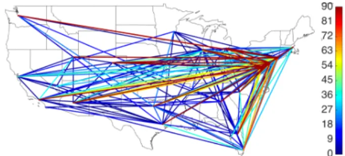
Delay networks are useful representations and give a snap-shot of the entire system. We can also calculate the airport delay from the delay network. For example in Fig. 1, the airport delay of Dallas Fort Worth (DFW) is 1+5₂ = 3 min. A real example of a delay network is Fig. 2, which shows all the OD-pair delays on September 7, 2011 at 12 pm Eastern Standard Time. For ease of visualization, the directed edges are averaged out and there is only one line between the airports. We can clearly see in the figure that the northeast US is experiencing high delays. Any day can be represented as a sequence of delay networks. More precisely, a day is a time series of 24 delay networks (i.e., one for each hour).

Fig. 2: Delay state of the US airspace on 7 Sept 2011, at 12 pm. The color denotes the average departure delay of flights on each link (in min).

A. Problem statement

With these definitions, we identify the following delay prediction problems:

1) Classification of OD-pair delays: In this case, we predict whether or not the delay on an OD-pair, ∆t hours in the future, will exceed a pre-specified delay value (henceforth referred as the threshold). ∆t is the prediction horizon, namely, the number of hours into the future for which the prediction is made. The resulting problem is one of classification, in which we want to associate the future delay with one of the two categories (or classes): ‘above threshold’ or ‘below threshold’. A range of prediction horizons (from 2-24 hr), along with different classification thresholds (30 min, 60 min, 90 min) will be considered.

2) Prediction of OD-pair delays: Here, we predict the OD-pair delays, time ∆t hours in the future. By contrast to the classification problem, the actual value of OD-pair delays (in minutes) are predicted here, and not just whether or not the delay is above a threshold. In other words, this is a regression problem.

3) Prediction of airport delays: Similar to the OD-pair delay prediction, we predict the delay value for an airport, ∆t hours into the future. Once again, a range of prediction horizons, from 2-24 hr, are considered.

III. PREDICTIONMETHODOLOGIES

We compare several classes of methods for solving the clas-sification and regression problems. For the first method, Arti-ficial Neural Networks, we use standard network architectures for both the regression and classification problems. The second method is a classical technique from the machine learning literature: Classification and Regression Trees (CARTs). The third method, standard linear regression, is applicable only to the regression problems. Finally, we present a Markov Jump Linear System (MJLS) model, and demonstrate its applicability for both the OD-pair and airport delay regression problems.

Feature selection is a key aspect of machine learning prob-lems, and greatly influences the performance of the algorithms. Therefore, we first describe in detail the feature vectors that are used to train the different classes of models.

A. Feature vectors

With the exception of the MJLS model, all the methods we consider in this paper are supervised learning algorithms. This means that when they are trained, they are presented with input-output mappings, and the model learns appropriate parameters from these training samples. For the classification problem, the output is a binary (0-1) vector; for the regression problems, it is either the OD-pair delay or the airport delay.

The input presented to train the model, called the feature vector, can be selected in multiple ways. We first describe the different feature vectors that are used for the OD-pair classification and regression. Then, we present the feature vectors that are used for the airport delay regression. The

notation used is as follows: At time t, the delay at time (t + ∆t) needs to be predicted. In other words, the feature vectors can only use information that is known at or before t.

1) Feature vectors for OD-pair regression and classifica-tion: These following are factors that are considered for the OD-pair classification and regression problems.

• Time of day: Delays show temporal patterns. They tend to be small or zero between midnight and 6 am, and start increasing in the morning. By noon, most OD-pairs have a non-zero delay because of high traffic and associated congestion. External factors like weather also cause delays during the day. They tend to peak towards the evening, when congestion effects are the highest, and finally trail off at night once traffic decreases. Therefore, the time of day is an important feature.

• Day of week: Traffic, and consequently delay patterns, depends on the day of the week, making it a potential feature [18, 14, 19].

• Season: Since weather disruptions exhibit seasonality, the year is grouped into seasons based on the delays. • OD-pair delays: In addition to the current OD-pair delay,

the progression of OD-pair delays (for example, the delay for the past 2 hours), is an important indicator of delay trends. A high delay at 4 pm on the JFK-SFO link may indicate that the situation will worsen by 6 pm, when demand peaks.

• Delays on adjacent OD-pairs: Since delays tend to propagate in the network [20, 21, 22, 6], the delay on a particular OD-pair is influenced by those on adjacent OD-pairs (Fig. 3). This feature is most important for short prediction horizons, but for longer horizons, delays on non-adjacent links could also become important.

O D

Fig. 3: The dotted edges are adjacent links to the solid line OD-pair.

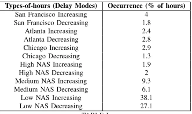
• Type-of-hour (delay mode): While the adjacent OD-pair delay is a local property, the type-of-hour or delay mode is a more global, network centric measure of the delay. Characteristic delay modes are identified by clustering delay networks [23]. These modes are also categorized depending on whether they are associated with increasing or decreasing delay trends. Each hour is associated with a delay mode (Table I) and a representative delay network. Prior work has also used the delay mode as a feature in delay prediction [13]. This feature incorporates the effect of weather conditions (like IMC or VMC) on the network delay.

• Type-of-day: Delay effects of one day may persist and affect the next day. The type-of-day variable captures this effect by grouping days into one of six categories based on the sequence of delay networks for the day [23]. Since

Types-of-hours (Delay Modes) Occurrence (% of hours)

San Francisco Increasing 4

San Francisco Decreasing 1.8

Atlanta Increasing 2.4

Atlanta Decreasing 2.8

Chicago Increasing 2.9

Chicago Decreasing 1.3

High NAS Increasing 1.9

High NAS Decreasing 2

Medium NAS Increasing 9.3

Medium NAS Decreasing 6.1

Low NAS Increasing 38.1

Low NAS Decreasing 27.1

TABLE I DELAY MODES IN2011-12.

the type-of-day for the current day may not be known at the time of making the prediction, the previous type-of-day variable is used.

In summary, we have three temporal variables (time, day of week and season), two local delay variables (OD-pair delay and adjacent OD-pair delay) and two network delay variables (delay mode and type of day). Using these features, we create 7 candidate feature vectors that are used for OD-pair delay classification and prediction. The different vectors incorporate different factors. We study the importance of these factors by studying the performance of prediction algorithms on different feature vectors.

F1 = [OD-Delay(t)] F2 = [OD-Delay(t), t]

F3 = [OD-Delay(t), t, day-of-week, season]

F4 = [OD-Delay(t), t, day-of-week, season, type-of-hour, previous type-of-day]

F5 = [OD-Delay(t), OD-Delay(t − 1), OD-Delay(t − 2)] F6 = [OD-Delay(t), type-of-hour, t]

F7 = [OD-Delay(t), Delay on adjacent OD-pairs(t), t] The feature vectors for the airport delay prediction include the airport delay variable instead of the OD-pair delays.

˜

F1 = [Airport delay(t)] ˜

F2 = [Airport delay(t), t] ˜

F3 = [Airport delay(t), Airport delay(t − 1), t] ˜

F4 = [All airport delays(t), previous type-of-day, t] B. Artificial Neural Networks (ANN)

We consider three architectures for the ANN, based on standard models [16, 15, 24].

N1: Multilayer Perceptron. This is also referred to as a feed-forward net. The network has an input layer, one or more hidden layers, and an output layer. We use two hidden layers with 10 perceptrons each, since we there was little performance improvement from adding more perceptrons or layers. The input and the hidden layers use a logistic activation function. The output layer uses a linear transfer function so that the range out of the output is (−∞, ∞). The architecture N1 can be used for regression as well as for classification. When N1 is used for regression, the output layer has just one neuron that gives the value of

the delay. For the classification problem, there are two output neurons representing the two classes, ‘delay above threshold’ and ‘delay below threshold’, respectively. N2: General Regression Neural Network. This is an efficient,

1-pass learning architecture that employs radial basis functions [25] for regression problems.

N3: Probabilistic Neural Network (PNN). These have a layer of neurons with radial basis functions, and a final compet-itive layer that is used for classification. In the competcompet-itive layer, the input neurons ‘compete’ amongst themselves and only one output class is activated. A more detailed discussion of PNNs can be found in [26].

C. Classical machine learning approaches

1) Classification and Regression Trees (CART): Decision trees map input vectors (or observation variables) to target values in the leaves. The branches split the input observation based on the observation value (the elements in the input vector) and this process is recursively done till we reach the leaves. In a Classification Tree (CT), the leaves represent one of the classes. In this paper, it will represent either a ‘delay above threshold’ or a ‘delay below threshold’ class. When the leaf represents the value of a continuous variable, it is called a Regression Tree (RT) [27].

2) Linear Regression (LR): In the linear regression model, the output is a linear combination of the input variables. The output in this paper would be the OD-pair delay, or the airport delay. The input variables could be continuous or categorical (like the time of day or season) and we use standard techniques to learn the coefficients.

D. Markov Jump Linear System (MJLS)

We briefly describe the MJLS model of airport delay dynamics [28]. Persistence of delays and network interactions are assumed to determine the airport delay. So for any air-port i, the outbound airair-port delay at time t + 1 is given as xout

i (t + 1) = αixouti (t) + ∑jβjiajixinj(t). The first term captures the persistence of delays and the second term captures the network interactions. ai j is the weight on link (i, j), and αi j, βi j are proportionality constants. Denoting the in-delay and out-delay of all airports using a state vector x(t), we have x(t + 1) = Γ(t)x(t), where Γ(t) = [α] + [β ]A(t) and A(t) is the adjacency matrix for the delay network. Instead of using A(t), which changes with time, we use the adjacency matrices for the characteristic delay modes (as shown in Table I). So for example, at a particular time t, the system might be in the ‘San Francisco decreasing’ delay mode, meaning that delays are primarily concentrated at San Francisco, and are decreasing in time. This leads to a linear dynamical system that is dependent on the current mode. m(t) denotes the delay mode of the system at time t. Each delay mode has a characteristic delay network that describes it, denoted by the adjacency matrix Am. Thus,

x(t + 1) = Γm(t)x(t) (1) At time step t + 1, i.e., the next hour, the system may remain in the same delay mode or transition to another. These

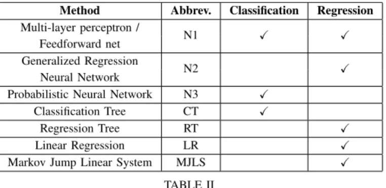
Method Abbrev. Classification Regression Multi-layer perceptron / N1 X X Feedforward net Generalized Regression N2 X Neural Network

Probabilistic Neural Network N3 X

Classification Tree CT X

Regression Tree RT X

Linear Regression LR X

Markov Jump Linear System MJLS X

TABLE II

SUMMARY OF THE DELAY PREDICTION TECHNIQUES FOR THEOD

CLASSIFICATION ANDOD/AIRPORT REGRESSION.

are modeled as a time-dependent Markovian transitions. For instance, because of the frequent occurrence of fog in San Francisco in the mornings, the probability of transitioning into the ‘SFO increasing’ delay mode is higher in the morning than at 6 pm. The transition probability is defined as

P[m(t + 1) = j|m(t) = i] = πi, j(t) (2) Eqs. (1)-(2) define the MJLS model. Fig. 4 shows a schematic of the MJLS, in which delays evolve according to the Mode 1 dynamics from time t0 to t1, then transition to Mode 2, and evolve according to the Mode 2 dynamics until t2.

Fig. 4: Schematic of the MJLS model.

The delay modes, transition matrices, and coefficients α and β are learnt from data. The model can directly be used for airport delay prediction. The characteristic delay modes (described using the networks Am) are used for OD pair delay prediction. If the current mode is known, the transition probability gives a future mode distribution. A probability weighted average of Amgives an estimate of the OD pair delay on all links.

IV. MODELEVALUATION

The methods developed in the previous sections are now evaluated using operational flight delay data. The details of the data set are first described, followed by the evaluation results.

A. Data sets

We use the Bureau of Transportation Statistics (BTS) data for 2011 and 2012 [2]. The data contains the delay values for all flights of commercial airlines that accounted for at least 1%

of the passenger traffic. The delay networks are constructed by considering only those links on which there are at least 5 flights a day, on an average. If there are multiple flights on an OD-pair, then the delay state of that link at hour t is taken to be the median departure delay of the flights taking off between tand t + 1 hour. In this manner, we obtain delay networks for each hour of the day, for the two years. The network contains 1,107 OD-pairs and 158 airports. We derive three sets of delay data from this ‘master set’ in order to study the performance of our prediction algorithms.

Dataset A: This set was used to evaluate the performance of the OD-pair delay classifier and delay level predictor. Data from 2011 was considered for training, and data from 2012 for testing. For each OD-pair, only those data points in which a) delay was non-zero and b) not during overnight hours, i.e., midnight-9 am EST (U.S. Eastern Standard Time), were included. Thereby only periods of non-zero traffic are considered, and outliers were removed. The performance of our algorithms on Dataset A are, for a practical prediction scenario, the most relevant. Unless stated otherwise, the results presented in this section refer to Dataset A.

Dataset B: This set was used to evaluate the performance of the OD-pair delay classifier and the delay level predictor under more challenging conditions. This data set is balanced, meaning that there are an equal number of high- and low-delay data points. For every OD-pair and a given classification threshold, say 60 min, half the data points have the OD-pair delay above 60 min and the other half has a delay of less than 60 min. All the points with delay above the threshold are chosen (since they are typically fewer in number), and the low delay points are chosen at random. The number of data points differ by OD-pair, since they each experience different durations of high delay periods (or non-negative delay periods). It is important to note that the data points in Dataset A and Dataet B have no time ordering – consecutive data points could be from time instants that are months apart. The prime motivation for the Dataset B is to evaluate classifier performance, but we still use it (with a 60 minute threshold) for the OD-pair regression problem for completeness.

Dataset C: This is used for evaluating the aggregate airport delay predictions. The FAA Core 30 airports, which are airports with high passenger traffic are considered (refer to Table V for the complete list). For each airport, all time periods where traffic is non-zero and the time is between 9 am and midnight EST are considered. Data from 2011 is used for training, and 2012 for testing.

B. Classification of OD-pair delays

1) 60 min classification threshold and 2 hr prediction horizon: For every OD-pair in Dataset A, we train them using the neural network architecture N1 and feature vector F1. The accuracy of classifying the delay on the link as above or below 60 min, with a 2-hr prediction horizon, is shown in Fig. 5. The OD-pairs are sorted by increasing prediction accuracy. The prediction accuracy varies from 84% to 99%. The average accuracy of using a multi-layer perceptron neural

network (N1) with feature vector F1 is 93.6%. The accuracy of the other methods, with feature vectors F1-F7, are shown in Fig. 6.

OD pair index (sorted)

0 20 40 60 80 100 Accuracy (percentage) 84 86 88 90 92 94 96 98 100

Fig. 5: Accuracy for predicting OD-pair delays, for a classi-fication threshold of 60 min and prediction horizon of 2 hr, using neural net N1, and feature F1.

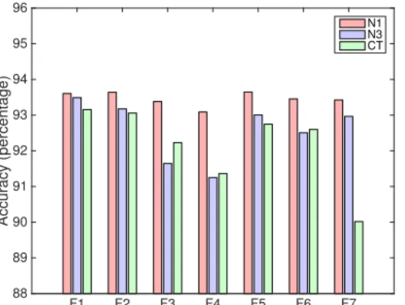
F1 F2 F3 F4 F5 F6 F7 Accuracy (percentage) 88 89 90 91 92 93 94 95 96 N1 N3 CT

Fig. 6: Comparison of neural net N1, N3 and classification tree (CT) with features F1-F7, for 2-hr classification of OD-pair delays, with a threshold of 60 min.

The architecture N1 is consistently the best performer among the three methods, with an accuracy of over 93%. In fact, the highest accuracy of 93.7% among all the methods was with network N1 and feature F2. The feature vector F5 which contains Information about the delay trend (it includes delay at t, t − 1 and t − 2) is very close, with an accuracy of 93.6%. It is interesting that the accuracy of the neural network does not change significantly based on the features, and that the addition of network information in F4 does not improve the accuracy of any method. N1 has a small decrease in performance, whereas N3 and CT are significantly worse. Finally, the feature F6, which includes delays from adjacent OD-pairs also gives limited improvement to the neural nets, and worsens the performance of the CT. For this prediction problem, the neural network architectures outperform CT.

2) Effect of classification threshold: We use architecture N1 with feature vector F2, since it was the best performing method, in order to study the variation of accuracy with

classification threshold. We consider 30 min, 60 min and 90 min classification thresholds.

OD pair index (sorted)

0 20 40 60 80 100 Accuracy (percentage) 60 65 70 75 80 85 90 95 100 60 Min 30 Min 90 Min

Fig. 7: Accuracy of OD-pair delay classification with a thresh-old of 30, 60 and 90 min, and prediction horizon of 2 hr, using neural net N1 with feature F2.

Fig. 7 shows that for the same OD-pair, accuracy increases as the classification threshold increases. In particular, the average accuracy is 85% for a 30 min threshold, 94% for a 60 min threshold, and 97% for a 90 min threshold. Intuitively, it is easier to predict whether the delay will exceed 90 min, than exceed 30 min, since such high delays will usually be preceded by cues such as increasing delay trends. Prediction with smaller thresholds is harder because of noise and other random fluctuations. It is worth noting that the U.S. Department of Transportation only counts a flight as being delayed if its delay exceeds 15 minutes.

3) Effect of prediction horizon: When the prediction hori-zon is increased from 2 hr to 4 hr, 6 hr, or 24 hr, the accuracies shown in Fig. 6 decrease by less than 1%. The most accurate prediction technique remains N1 with the use of F2. However, there is an increase in the accuracy to 95% (CT with F2) when the prediction horizon is reduced to 1 hr.

4) Analysis with Dataset B: Dataset A is not a balanced dataset. While the accuracy of the best algorithm for a 2 hour prediction with a 60 minute threshold is 93.7%, even a naive classifier which always predicts a delay below the threshold will give an accuracy of 93.5%. On training and testing the algorithms using the balanced Dataset B, the classification accuracy of the best algorithm is 71% (Tab. III). This is a more rigorous statistical analysis of the algorithms, and gives context to the accuracy: a naive classifier, which classifies all data points into any one type, will be only be 50% accurate in this case. This demonstrates the benefits of using the the specialized prediction techniques.

C. Estimation of OD-pair delays

The OD-pair delay is predicted using neural nets N1 and N2, a regression tree (RT), linear regression (LR) and the Markov Jump Linear System (MJLS) model. The prediction error for an OD-pair is the median of the absolute error across all the data points in the test set (the year 2012). The prediction error

N1 N3 CT F1 66.6 66.7 67.2 F2 69.0 68.9 70.6 F3 64.2 60.6 69.4 F4 64.0 52.5 69.5 F5 65.7 66.2 67.1 F6 66.5 64.3 70.2 F7 67.5 50.1 70.0 TABLE III

ACCURACY(%)OF DIFFERENT METHODS,FOR A2HR PREDICTION AND A

60MIN CLASSIFICATION THRESHOLD,USINGDATASETB.

for a method is defined as the mean prediction error over all the 100 OD-pairs.

1) Comparison of methods: For a 2 hr prediction horizon, the MJLS model has the lowest prediction error of 4.7 min. Among the other methods, the neural net N2 with feature F7 gives the lowest error of 8.4 min (Fig. 8). To place these errors in context, it is important to compare them to the mean error across all OD pairs in the test set, which is 7.2 min. The

F1 F2 F3 F4 F5 F6 F7

Prediction error (min)

7 8 9 10 11 12 13 14 N1 N2 RT LR

Fig. 8: Average prediction error (in min) over 100 OD-pairs for a 2 hr prediction horizon. Neural networks (N1 and N2), Regression Tree, and Linear Regression, with feature vectors F1-F7 are considered.

Generalized Regression Neural Network (N2) is the better performing neural network, and it is marginally better than the Regression Tree. The delays on all adjacent links (F7) is a more significant feature than the network-theoretic features like previous type-of-day or type-of-hour (F4 and F6). This makes intuitive sense, because in the short term (i.e., 2 hr), an OD-pair delay is unlikely to be affected by delay on links that are more than one hop away. The error for N2 is, however, almost 80% more than the MJLS. This reflects the inability of the neural network to extract out complex features like the principal eigenvector, which form the basis for the modes in the MJLS model.

The distribution of prediction error for each of the 100

OD-pairs (Fig. 9) shows a peak for the MJLS model at lower delay values. The tail of the distribution is longer for the Regression Tree, with the prediction error being as high as 25 min for one of the OD-pairs.

0 20 40 60 N2 Number of OD pairs 0 20 40 60 RT

OD-pair delay error (min)

0 5 10 15 20 25 30 0 20 40 60 80 MJLS

Fig. 9: Distribution of OD-pair delay prediction errors for N2 and RT (both with feature F7), and the MJLS model.

2) Effect of prediction horizon: The trend of MJLS being the best prediction model followed by N2 and RT (both with feature F7) holds for a prediction horizon of 4 hr, 6 hr, and 24 hr (Fig. 10).

Prediction Horizon

2 hr 4 hr 6 hr 24 hr

Prediction error (min)

3 4 5 6 7 8 9 10 11 12 N2 with F7 RT with F7 MJLS

Fig. 10: Distribution of OD-pair delay prediction errors for N2, RT, and MJLS, for a 2 hr, 4 hr, 6 hr and 24 hr prediction horizon

3) Analysis with Dataset B: With the balanced Dataset B, it is natural that the prediction errors will increase. While most models and feature vectors show an increase by a factor of 3 (Tab. IV), the N2 architecture with the F7 feature vector is robust and predicts the delay with an average error of 18.5 min. The MJLS model has an error of 44 min, and is not the best algorithm. With a lot of high delay data points in this set, a simple (although it is reasonably powerful, as seen with Dataset A) MJLS model is not able to capture the complex nonlinear delay dynamics that govern these high delay instances. The neural network performs much better in

N1 N2 RT LR F1 42.2 39.4 39.4 44.2 F2 36.1 32.1 30.9 32.6 F3 44.9 36.0 31.1 34.9 F4 46.1 32.4 33.8 45.9 F5 44.0 37.6 37.4 43.5 F6 39.7 31.0 30.1 33.8 F7 42.6 18.5 29.5 77.54 TABLE IV

MEANOD-PAIR DELAY PREDICTION ERROR(IN MIN)FOR2HR PREDICTION HORIZON WITHDataset B. FOR COMPARISON,THEMJLS

MODEL HAS A MEAN ERROR OF44MIN.

such situations. In this balanced dataset, the mean of the delay that is being predicted is 50.7 min.

D. Estimation of airport delays

The airport delay regression is used to predict the average delay levels of outgoing links from an airport. This is a measure of the delay disruptions, or the quality of service at the airport.

1) Comparison of methods: We use the neural networks N1 and N2, a Regression Tree (RT), a Linear Regression (LR) and the MJLS model to predict the delay state of an airport. The feature vectors are ˜F1- ˜F4, as described in Sec. III-A. For the MJLS, the current time, mode and the current delay at all airports is the feature. For each of the 30 airports in the FAA Core 30 list, the airport delay 2 hr in the future is predicted. The prediction error for an airport is the median error across all the data points. The average prediction error across all the 30 airports is defined as the prediction error for the particular algorithm (for the corresponding feature vector). Fig. 11 shows the average prediction error for the different algorithms. The error for the MJLS model (not shown in the plot) is 6.8 min, and it is the lowest among all the models. The mean of the airport delays in the test data set is 14.7 min.

˜

F 1 _{F 2}˜ _{F 3}˜ _{F 4}˜

Prediction error (min)

6 6.5 7 7.5 8 8.5 9 9.5 10 N1 N2 RT LR

Fig. 11: Comparison of all models for a 2 hr prediction of airport delay. The MJLS model (not shown) results in a prediction error of 6.8 min.

Among the models compared in Fig. 11, the neural network

N1 (with feature ˜F2), which is a multi-layer perceptron network gives the lowest error of 7.1 min. The neural net-work outperforms the other classical techniques of Regression Tress and Linear Regression for the airport delay prediction; however, it does not perform as well as the MJLS. The MJLS model incorporates network effects and temporal dynamics (through the time-dependent transition matrices). It is not possible for the neural network to learn all temporal features because it treats each data point independently as a new observation, and not as a time-series. However, the neural network model is simpler, and can be developed without any assumptions or intuition about the delay dynamics. We also observe that feature vectors F2 and F3, which contain temporal information, give better performance with neural network N1 than feature F4, which contains network effects (previous type-of-day). For predictions only 2 hr into the future, the current dynamics is a more important factor than the network state of the previous day.

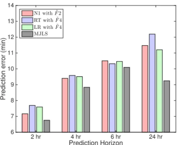
2) Effect of prediction horizon: For prediction horizons of 2, 4, 6, and 24 hr, the MJLS had the lowest prediction error among all the models. Among the other models, the lowest error is obtained by neural network N2 (for 2 and 4 hr predic-tion horizons), Regression Tree (for a 6 hr predicpredic-tion horizon) and Linear Regression (for a 24 hr prediction horizon). The performance of these four methods are plotted in Fig. 12.

Prediction Horizon

2 hr 4 hr 6 hr 24 hr

Prediction error (min)

6 7 8 9 10 11 12 13 14 N1 with ˜_{F 2} RT with ˜_{F 4} LR with ˜_{F 4} MJLS

Fig. 12: N2, RT, LR and MJLS prediction errors of airport delays, for 2 hr, 4 hr, 6 hr, and 24 hr prediction horizons.

While the neural network is better for lower prediction hori-zons, RT and LR become better for longer horizons. Feature

˜

F4, i.e., the previous type-of-day, becomes more useful at longer prediction horizons. The local dynamics at t and t − 1 are intuitively not very useful when a prediction needs to be made at t + 24. The superior performance of the MJLS model highlights the importance of specialized, physically interpretable models. Naturally, the MJLS prediction error will increase with increasing prediction horizons. This can be ascribed to the increasing uncertainty about the delay dynamics over longer time scales. However, the prediction error for the 24 hr horizon is lower than the 6 hr horizon. This apparent anomaly is due to the distribution of our data

Airport Delay (min) Prediction error (min) Median IQR 2 hr 4 hr 6 hr 24 hr ATL 11.4 15.0 3.4 4.6 6.03 5.7 BOS 13.5 28.7 7.1 9.7 10.9 9.7 BWI 20 32.1 8.4 11.5 13.2 12.0 CLT 12.8 27.5 6.0 7.5 8.5 7.5 DCA 10.3 22.4 6.6 8.8 10.2 9.0 DEN 16.4 21.0 4.3 5.4 6.4 7.4 DFW 16.3 20.2 5.0 7.0 8.4 7.7 DTW 16.3 35.1 8.3 10.8 12.2 11.5 EWR 25.3 44.3 9.8 12.6 15.1 14.4 FLL 14.5 31.2 8.6 11.6 13.2 11.7 HNL 2.5 6.9 2.7 3.4 3.7 3.0 IAD 28.3 53.6 12.9 16.4 17.2 16.6 IAH 20.9 31.7 7.3 9.6 11.4 10.8 JFK 17.1 29.6 8.5 11.2 12.6 10.7 LAS 14.0 19.5 4.4 5.4 6.3 6.6 LAX 13.8 15.9 4.0 4.8 5.8 6.4 LGA 9.5 25.6 6.0 8.0 9.1 7.4 MCO 15.1 28.1 6.9 8.6 9.6 9.2 MDW 19.9 30.4 7.4 10.0 12.0 11.6 MEM 3.0 22.0 9.6 14.3 16.2 10.9 MIA 22.3 32.1 9.7 11.7 12.8 13.3 MSP 12.0 26.7 8.1 10.4 11.3 9.6 ORD 18.5 29.4 5.2 7.1 8.9 8.8 PHL 12.3 23.7 8.6 11.3 12.2 10.4 PHX 12.2 15.1 3.7 4.5 5.1 5.6 SAN 10.3 17.1 5.2 6.0 6.5 6.2 SEA 11.3 15.4 4.8 6.0 6.6 5.7 SFO 20.9 36.4 6.3 8.4 10.3 10.4 SLC 10.3 18.6 5.6 6.5 7.2 6.0 TPA 11.4 29.7 8.3 11.5 13.5 11.3 TABLE V

MEDIAN DELAY AND THEINTERQUARTILERANGE(IQR)FOR EACH AIRPORT,ALONG WITH THE AIRPORT DELAY PREDICTION ERRORS FOR2, 4, 6,AND24HR HORIZONS ONDataset C,USING THEMJLSMODEL. THE

IQRIS THE DIFFERENCE BETWEEN THE25TH AND75TH PERCENTILES. ALL QUANTITIES ARE IN MINUTES.

points. When making a 6 hour prediction, the MJLS uses delay at 4 am to predict the delay at 10 am. Since the model is multiplicative on the initial condition, it is extremely sensitive to the low delay, and fluctuations that are characteristic of a 4 am delay. On the other hand, when 24 hr predictions are made, delays during high traffic periods are used to make predictions. There is also valuable information about the previous type of day that is used, which explains why the error drops despite the increase in prediction horizon. The neural network and other models are not multiplicatively dependent on the initial state, and therefore do not exhibit such behavior. Finally, the median MJLS prediction error, as well as the median delay, by airport is shown in Table V.

E. Discussions

It is apparent that the best choice of delay prediction method depends on (1) the specific classification or regression problem, (2) the dataset (balanced vs. unbalanced), and (3) the prediction horizon.

For the classification problem at a 2 hr prediction horizon and 60 min threshold, we achieved a 94% accuracy, for

Dataset A. For the balanced dataset, the accuracy dropped to 70%. Similar accuracy was achieved in [13] using the time-of-day as a prediction variable. However, by using other network delay states and random forests, they were able to achieve a much higher accuracy. This result suggests that ensemble methods using artificial neural networks may be an interesting topic for further study.

For the OD-pair regression problem, the MJLS model per-formed the best when considering Dataset A. The identification and effective use of spatial delay patterns (delay modes), and the temporal evolution (time-dependent mode transitions), makes the MJLS model a very good predictive tool, with a mean error of 4.7 min. However, when a balanced data set was used, the neural network became the best performer with an OD-pair error of 18.5 min. The MJLS model is not appropriate to use for Dataset B, since the model development used the entire 2011 data points (and not the balanced data set) to identify significant delay modes. The closest point of comparison would be [13], where a Random Forest algorithm on a 2007-08 ASPM dataset had an error of 21 min, for a 2 hr prediction horizon.

The airport delay metric has not been predicted in prior literature. We hypothesize that ensemble methods (like random forests) would help boost the accuracy of neural network methods. However, they may still not be as accurate as MJLS, because of the specialized dynamical features that are explicitly accounted for by the MJLS model.

V. CONCLUSIONS

We compared the performance of several algorithms for delay prediction (ANN, MJLS, CART, LR). Temporal (time-of-day, day-of-week, season), local (airport delay, OD-pair delay) and network (type-of-hour, type-of-day) factors were used to make these predictions. While the ANN performed well for OD-pair delay classification (mean error: 94% for 60 min threshold and 2 hr horizon), the MJLS gave the least error for the OD-pair delay regression (mean error: 4.7 min for 2 hr horizon) and airport delay regression (mean error: 6.8 min for 2 hr horizon) problems. Even for a 24 hr prediction horizon, the MJLS could predict OD-pair delays with a mean error of 4.7 min, and airport delays with a mean error of 9.2 min.

The importance of features also differed by problem and prediction horizon. For instance, the time-of-day was the most important factor driving the accuracy of OD-pair delay classi-fication. However, for the OD-pair delay regression problem, time-of-day became less important at longer prediction hori-zons, and network factors (type-of-day) gained prominence. These observations give us valuable insights into feature selection. Finally, these results serve as a valuable baseline for delay prediction algorithm refinements that account for weather disruptions and Traffic Management Initiatives such as Ground Delay Programs.

REFERENCES

[1] Airports Council International, “2015 World Airport Traffic Report,” 2016.

[2] Bureau of Transportation Statistics, “Airline On-Time Statistics and Delay Causes,” 2015. [Online]. Available: http://www.transtats.bts.gov/

[3] Joint Economic Committee, US Senate, “Your Flight has Been Delayed Again: Flight Delays Cost Passengers, Airlines, and the US Economy Billions,” 2008.

[4] M. Ball, C. Barnhart, M. Dresner, M. Hansen, K. Neels, A. Odoni, E. Peterson, L. Sherry, A. Trani, and B. Zou, “Total delay impact study,” 2010.

[5] N. Pyrgiotis, K. M. Malone, and A. Odoni, “Mod-elling delay propagation within an airport network,” Transportation Research Part C: Emerging Technologies, vol. 27, pp. 60–75, 2013.

[6] P. Fleurquin, J. Ramasco, and V. Eguiluz, “Systemic delay propagation in the US airport network,” Scientific Reports, p. 1159, 2013.

[7] K. Gopalakrishnan, H. Balakrishnan, and R. Jordan, “Deconstructing Delay Dynamics: An air traffic network example,” in International Conference on Research in Air Transportation (ICRAT), 2016.

[8] M. Zanin and F. Lillo, “Modelling the air transport with complex networks: A short review,” The European Physical Journal Special Topics, vol. 215, pp. 5–21, 2013.

[9] Y. Tu, M. O. Ball, and W. S. Jank, “Estimating flight departure delay distributions- a statistical approach with long-term trend and short-term pattern,” Journal of the American Statistical Association, vol. 103, no. 481, pp. 112–125, 2008.

[10] A. Klein, S. Kavoussi, D. Hickman, D. Simenauer, M. Phaneuf, and T. MacPhail, “Predicting Weather Im-pact on Air Traffic,” in Integrated Communication, Nav-igation and Surveillance (ICNS) Conference, May 2007. [11] A. Klein, C. Craun, and R. S. Lee, “Airport delay prediction using weather-impacted traffic index (WITI) model,” in Digital Avionics Systems Conference, 2010. [12] N. Xu, K. B. Laskey, G. Donohue, and C. H. Chen,

“Es-timation of Delay Propagation in the National Aviation System Using Bayesian Networks,” in 6th USA/Europe Air Traffic Management Research and Development Sem-inar, June 2005.

[13] J. J. Rebollo and H. Balakrishnan, “Characterization and prediction of air traffic delays,” Transportation Research Part C, pp. 231–241, 2014.

[14] Z. J. Hanley, “Delay Characterization and Prediction in Major U.S. Airline Networks,” Master’s thesis, Mas-sachusetts Institute of Technology, 2015.

[15] C. M. Bishop, Pattern Recognition and Machine Learn-ing (Information Science and Statistics). Secaucus, NJ, USA: Springer-Verlag New York, Inc., 2006.

[16] H. B. Demuth, M. H. Beale, O. De Jess, and M. T. Hagan, Neural network design. Martin Hagan, 2014.

[17] Y. J. Kim, S. Choi, S. Briceno, and D. Mavris, “A deep learning approach to flight delay prediction,” in Digital Avionics Systems Conference (DASC), 2016 IEEE/AIAA

35th. IEEE, 2016, pp. 1–6.

[18] E. Mueller and G. Chatterji, “Analysis of aircraft arrival and departure delay characteristics,” in AIAA’s Aircraft Technology, Integration, and Operations (ATIO) 2002 Technical Forum, 2002, p. 5866.

[19] J. J. Rebollo and H. Balakrishnan, “A network-based model for predicting air traffic delays,” in 5th Interna-tional Conference on Research in Air Transportation, 2012.

[20] P. Fleurquin, J. Ramasco, and V. Eguiluz, “Data-driven modeling of systemic delay propagation under severe meteorological conditions,” in 11th USA/Europe Air Traf-fic Management Research and Development Seminar (ATM2011), Lisbon, Portugal, June 2015.

[21] M. Jetzki, “The propagation of air transport delays in Europe,” Master’s thesis, Department of Airport and Air Transportation Research, Aachen University, 2009. [22] S. AhmadBeygi, A. Cohn, Y. Guan, and P. Belobaba,

“Analysis of the Potential for Delay Propagation in Passenger Airline Networks,” Journal of Air Transport Management, vol. 14 No. 5, pp. 221–236, 2008. [23] K. Gopalakrishnan, H. Balakrishnan, and R. Jordan,

“Clusters and Communities in Air Traffic Delay Net-works,” in American Control Conference, July 2016. [24] N. K. Bose and P. Liang, “Neural network fundamentals

with graphs, algorithms and applications,” McGraw-Hill, 1996.

[25] D. F. Specht, “A general regression neural network,” IEEE transactions on neural networks, vol. 2, no. 6, pp. 568–576, 1991.

[26] ——, “Probabilistic neural networks,” Neural networks, vol. 3, no. 1, pp. 109–118, 1990.

[27] E. Alpaydin, Introduction to machine learning. MIT press, 2014.

[28] K. Gopalakrishnan, H. Balakrishnan, and R. Jordan, “Stability of networked systems with switching topolo-gies,” in Decision and Control (CDC), 2016 IEEE 55th Conference on. IEEE, 2016, pp. 2601–2608.

AUTHORBIOGRAPHY

Karthik Gopalakrishnan is a PhD candidate in the department of Aeronautics and Astronautics at the Massachusetts Institute of Technology. His research focuses on the application of optimization methods and control theory to analyze networked systems. He is a recipient of the best paper award at the International Conference on Research in Air Transportation (2016).

Hamsa Balakrishnan is an Associate Professor of Aeronautics and Astronautics at the Massachusetts Institute of Technology. Her research is in the design, analysis, and implementation of control and optimization algorithms for large-scale cyber-physical infrastructures, with an emphasis on air transportation systems. She is a recipient of the Donald P. Eckman Award from the American Automatic Control Council (2014), the Lawrence Sperry Award from the AIAA (2012), the CNA Award for Operational Analysis (2012), the best paper award at the ATM R&D Seminar (2011), and an NSF CAREER Award (2008).