Zsófia L. Bárány**, Christian Siegel***
By reviewing our work in Bárány, Siegel (2018a, 2018b), this article emphasizes the link between job polarization and structural change. We summarize evidence that job polarization in the United States has started as early as the 1950s: middle-wage workers have been losing both in terms of employment and average wage growth compared to low- and high-wage workers. Furthermore, at least since the 1960s the same patterns for both employment and wages have been discernible in terms of three broad sectors: low-skilled services, manufacturing and high-skilled services, and these two phenomena are closely linked. Finally, we propose a model where technology evolves at the sector-occupation cell level that can capture the employment reallocation across sectors, occupations, and within sectors. We show that this framework can be used to assess what type of biased technological change is the driver of the observed reallocations. The data suggests that technological change has been biased not only across occupations or sectors, but also across sector-occupation cells.
O
ver the last several decades the labor markets in most developed countries have experienced substantial changes. Since the middle of the twentieth century there has been structural change, the movement of labor out of manufacturing and into the service sectors. One of the key explanations for structural transformation is differential productivity growth –or biased technological progress– across sectors, combined with complementarity between the goods and services produced by different sectors* This article reviews findings of our previous joint work, and was prepared for the conference “Polarization(s) in Labor Markets” organized by the Direction de l’animation de la recherche, des études et des statistiques (DARES) and the International Labour Organization (ILO) in Paris on June 19, 2018.
** Zsófia Bárány, Sciences Po and Centre for Economic Policy Research (CEPR); [email protected]. *** Christian Siegel, University of Kent, School of Economics and Macroeconomics, Growth and History Centre; [email protected].
(ngai, PiSSarideS [2007]).1 At the level of occupations several papers have docu-mented the polarization of labor markets in the United States and in several European countries since the 1980s: employment has shifted out of middle-earning routine jobs to low-earning manual and high-earning abstract jobs. The main explanation for this phenomenon is the routinization hypothesis, which assumes that information and computer technologies (ICT) substitute for middle-skill, routine occupations, while they complement high-skill, abstract occupations; in other words technological pro-gress that is biased across occupations (autor et al. [2003], autor et al. [2006], autor, dorn (2013), gooS et al. [2014]). Both literatures –on structural change and polarization– study the impact of differential productivity growth. One focuses on the productivity across sectors and its interaction with the demand for goods and services, while the other focuses on the productivity of tasks or occupations, and its impact on the relative demand for these occupations. In this paper we review our previous work which suggests that these two phenomena are connected and should not be studied in isolation, especially in order to understand the driving forces behind the reallocation of labor across sectors and occupations.
In Bárány, Siegel (2018a) we show that polarization started much earlier than previously thought, and that it is closely linked to the structural transformation of the economy. This on its own suggests that there might be a common driving force behind structural transformation and polarization. In Bárány, Siegel (2018b) we go further; we demonstrate that there is an even tighter connection between the sectoral and occupational reallocation of employment, and we explicitly study the technological changes underlying both.
In Bárány, Siegel (2018a) we document first that in the US, occupational pola-rization both in terms of wages and employment has started in the 1950s, much earlier than suggested by previous literature. Second, we show that a similar polarization pattern is present for broadly defined sectors of the economy, low-skilled services, manufacturing, and high-skilled services. Moreover, we show that a significant part of the occupational employment share changes is driven by shifts of employment across sectors, and that sectoral effects also explain a large part of occupational wage changes. These findings suggest that the decline in routine employment is strongly connected to the decline in manufacturing employment. We propose a model to show that differences in productivity growth across sectors lead to the polarization of wages and employment at the sectoral level, which in turn implies polarization in occupational outcomes.
In Bárány, Siegel (2018b) we look at the data from a different perspective: we study employment patterns across sector-occupation cells in the economy. We document some trends in occupation and sector employment that have not received much attention in the literature. First, the manufacturing sector has the highest share of routine workers; 1. Some papers emphasize changes in the supply of an input which is used at different intensity across sectors (CaSelli, Coleman [2001], aCemoglu, guerrieri [2008]). Other papers study the role of non-homothetic preferences, where changes in aggregate income induce a reallocation of employment across sectors (KongSamut et al. [2001], BoPPart
by far most of the decline in routine employment has occurred in manufacturing, and conversely almost all of the contraction in manufacturing employment has occurred through a reduction in routine employment. Second, the high-skilled service sector has the highest share of abstract workers; most of the expansion in abstract employment has happened in the high-skilled service sector, and most of the increase in high-skilled service employment has been due to an expansion in abstract employment. These patterns reveal that the sectoral and the occupational reallocation of employment are closely linked. Furthermore, the overlap of occupations and sectors implies that it is hard to identify the technological changes which underlie the observed labor market patterns. To overcome this issue, we specify a flexible model of the production side of the economy in which technological change can be biased towards workers in specific sector-occupation cells. We use key equations of this model together with data from the US Census and from the U.S. Bureau of Economic Analysis (BEA) to draw conclusions about the bias in productivity changes across sector-occupation cells.
This approach departs from the recent literature connecting the phenomena of structural change and polarization across occupations in that we do not a priori res-trict the nature of technological change. gooS et al. (2014) suggest that differential occupation intensity across sectors and differential occupational productivity growth can lead to employment reallocation across sectors. duerneCKer, Herrendorf (2016) show in a two-sector two-occupation model that unbalanced occupational productivity growth by itself provides dynamics consistent with structural change and with the trends in occupational employment, both overall and within sectors. lee, SHin (2017) allow for occupation-specific productivity growth and find that their calibrated model can quantitatively account for polarization as well as for structural change, and in an extension find a limited role for sector-specific technological change. aum et al. (2018) analyze the role of routinization (differential productivity growth of occupations) and computerization across industries as well as industry-specific Total Factor Productivity (TFP) differences in the recent productivity slowdown, and find in their model with homogeneous labor that sectoral TFP differences have a rather small effect.
The close link in the data between the sectoral and occupational reallocation of labor explains why models which allow for productivity growth differences only at the sectoral or only at the occupational level can go a long way in accounting for the reallocations across both dimensions. However, such restricted models load all differences in technological change on one type of factor, therefore not allowing to identify whether these differences arise indeed at the level of sectors or of occupations. We view our framework as an important and useful first step in identifying the true bias in technological change. In this article we explain how certain aspects of the data can be used to draw qualitative conclusions, whereas in Bárány, Siegel (2018b) we use a richer methodology to quantify the bias in technology across sector-occupation cells and to decompose it further into common components. To summarize our results, we find that technological change has been biased in more nuanced ways, not just across occupations or sectors, but across sector-occupation cells.
A Historical Perspective on Polarization
In Bárány, Siegel (2018a) we use data from the US Census between 1950 and 2000 and the 2007 American Community Survey (ACS) to study the patterns of employment and wages both across occupations and across sectors. In the following three subsections we summarize the main empirical results we established there. Our main findings are the following: (1) occupational polarization both in terms of wages and employment started as early as 1950 in the US, (2) wage and employment polarization is also visible in terms of broadly defined industries, (3) a large part of polarization in terms of occupations is driven by changes at the level of industries. In the last subsection we go further and document the changes in employment at the sector-occupation cell level where we see a strong overlap between the evolution of occupational and sectoral employment trends.
Occupational Polarization
Figure 1 plots the smoothed changes in log real wages and employment shares for occupational percentiles, with occupations ranked according to their 1980 mean hourly wage, following the methodology used in autor et al. (2006), aCemoglu, autor (2011), and autor, dorn (2013) (Box 1). Departing from the literature, we do not restrict attention to recent years but show the changes starting from 1950 for different 30-year periods. The top panel shows that there has been (real) wage polarization throughout, as occupations towards the middle of the wage distribution have gained less than occupations at both extremes. The bottom panel shows that also in terms of their shares in hours worked, middle earning occupations have been tending to do worse than both low- and high-earning occupations. Though the pattern is less striking than for wages, polarization of employment has occurred since the 1950s.
Box 1
Ranking Occupations by Skill Level
Figure 1 –as is standard in the literature, e.g. autor et al. (2006), aCemoglu, autor (2011) and autor, dorn (2013)– shows smoothed changes in log real wages or in employment shares by percentiles of the occupational wage distribution, where occupations are ranked by their “skill level”, which is approximated by the average wage of workers in the given occupation in a base year. These occupations are then put into 100 bins on the horizontal axis, each representing 1 percent of employment. For such a comparison over time a balanced set of occupational codes are needed. In Bárány, Siegel (2018a) we construct the finest possible set of occupational codes that is balanced over 1950 to 2007, extending the work of meyer, oSBorne (2005) and dorn (2009).
To get a sense of which occupations are driving these changes and whether there are any significant differences across decades, in Figure 2 we show the decade-by-decade change in total hours worked and mean log wages for 10 coarser occupational categories. The categories we use follow aCemoglu, autor (2011), and are ranked
figure 1 – Smoothed Changes in Wages and Employment
Note: Balanced occupation categories (183 of them) have been defined by the authors based on meyer, oSBorne (2005), dorn (2009) and autor (2013). The horizontal axis contains occupational skill percentiles based on their 1980 mean wages. In the top panel the vertical axis shows for each occupational skill percentile the 30-year change in log hourly real wages, whereas in the bottom panel it shows the 30-year change in employment shares (calculated as hours supplied).
Source: Bárány, Siegel (2018a). The data is taken from IPUMS US Census data for 1950, 1960, 1970, 1980, 1990, 2000 and the
American Community Survey (ACS) for 2007. The sample excludes agricultural occupations/industries and observations with missing wage data. 1950-1980 1970-2000 1960-1990 1980-2007 0 20 40 60 80 100 –0.3 0 0.3 0.6 1.2 2.7 2.4 2.1 1.8 1.5 0.9
30-Yr Change in ln(real w
age)
Occupation’s Percentile in 1980 Wage Distribution
Change in Log Wage
1950-1980 1970-2000 1960-1990 1980-2007 0 20 40 60 80 100 –0.4 –0.3 –0.2 –0.1 0 0,1 0,2 0,3 0,4
30-Yr Change in Emplo
yment Share
Occupation’s Percentile in 1980 Wage Distribution
according to the occupations’ mean wages, from lowest earners on the left to highest earners on the right. Between 1950 and 1960 a clear pattern cannot be discerned, whereas from 1960 onwards, it is clear that both total hours worked and mean log wages have grown faster at both extremes than for occupations in the middle.
figure 2 – Polarization in Broad Occupational Categories
Source: Bárány, Siegel (2018a). The data used is the same as in Figure 1.
1950-1960 1960-1970 2000-2007 1970-1980 1980-1990 1990-2000 Personal Care –0.05 0 0.05 0.10 0.15 0.20 0.30 0.25
Food/Cleaning ServiceProtecti ve Service
Production Operators/Laborers Of
fice/AdministrationSales Technicians Professionals Managers
Percentage Change in Log Wages by Occupation, 1950-2007
1950-1960 1960-1970 2000-2007 1970-1980 1980-1990 1990-2000 Personal Care –0.5 0 0.5 1 1.5
Food/Cleaning ServiceProtecti ve Service
Production Operators/Laborers Of
fice/AdministrationSales Technicians Professionals Managers
Finally, following aCemoglu, autor (2011), we classify occupations into manual, routine and abstract categories.2 Figure 3 plots their paths of relative wages
and of employment shares. The top panel shows the path of occupational premia. These premia are the exponents of the coefficients on occupation dummies, obtained from a regression of log wages controlling for gender, race, a polynomial in potential experience, as well as occupation dummies. Obtaining the occupation premia from these regressions allows us to disregard changes in wage differences across occupations which are potentially caused by age, gender, or racial composition differences. It is worth to note that, as expected, the manual premium is less than the routine, while
2. See Box 2 for details of which 1-digit occupational codes are in each category.
Manual Abstract Routine
1950 1960 1970 1980 1990 2000 2010
0 0.2 0.4 0.6
0.8 Employment Shares of Occupations
figure 3 – Polarization for Broad Occupations
Source: Bárány, Siegel (2018a). Occupational wage premia and employment shares (in terms of hours) are calculated from the same data as in Figure 1. Manual Abstract 1950 1960 1970 1980 1990 2000 2010 0.50 0.75 1 1.25 1.75 1.50
the abstract premium is the largest. However, over time, the advantage of routine jobs over manual jobs has been falling, and the advantage of abstract jobs over routine jobs has been rising. The bottom panel shows that the employment share of routine occupations has been falling, of abstract occupations has been increasing since the 1950s, while that of manual occupations, following a slight compression until 1960, has been steadily increasing. Thus, the middle earning group, the routine workers, has lost both in terms of relative average wages and in terms of the employment share to the benefit of manual and abstract workers.
All these figures constitute evidence that at the occupational level there has been employment and wage polarization in the US since at least the 1960s.
Sectoral Polarization
Similar patterns can be discerned when considering the economy in terms of three broad sectors, low-skilled services, manufacturing, and high-skilled services (Box 2). As common in the structural change literature our manufacturing category includes mining and construction (e.g. as in Herrendorf et al. [2013]), whereas we split services in two (e.g. as in Buera, KaBoSKi [2012], duarte, reStuCCia [2017], duerneCKer et al. [2017]). Classification of economic activities into broad sectors for the purpose of a model should be such that industries within sectors are very good substitutes, while they are complements across sectors. Since the service sector as a whole includes very different types of services, by splitting it in two, we improve the analysis with regards to this criterion.
Box 2
Classification of Industries and Occupations
Industries are classified into our three categories as follows: low-skilled services are personal services, entertainment, low-skilled transport, low-skilled business and repair services, retail trade, and wholesale trade; manufacturing also includes mining and construction; high-skilled services are professional and related services, finance, insurance and real estate, communications, skilled business services, utilities, high-skilled transport, and public administration. In terms of occupations, manual workers are those working in: housekeeping, cleaning, protective service, food preparation and service, building, grounds cleaning, maintenance, personal appearance, recreation and hospitality, child care workers, personal care, service, healthcare support. Routine occupations are construction trades, extractive, machine operators, assemblers, inspectors, mechanics and repairers, precision production, transportation and material moving occupations, sales, administrative support. Finally abstract occupations comprise managers, management related, professional specialty, technicians and related support workers.
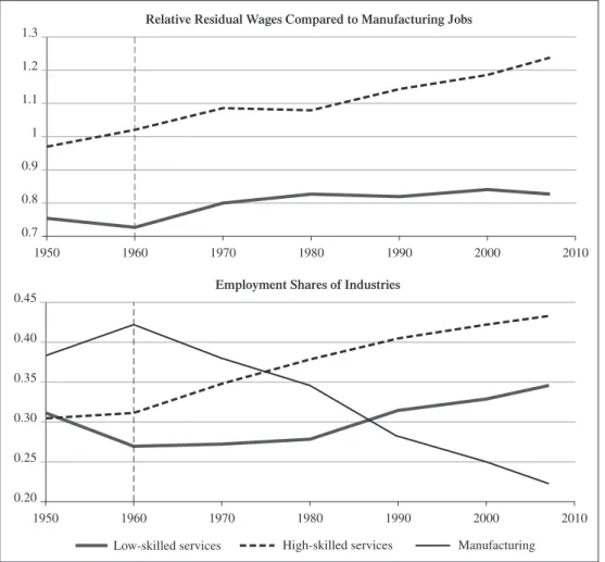
Figure 4 plots for these three sectors how wage premia and shares of hours worked have evolved over time. Similarly to the occupational premia, these sector premia are calculated from a Mincerian log wage regression as the exponents of the coeffi-cients on sector dummies, where we also control for gender, race, and a polynomial in potential experience. By construction, these sector premia do not contain changes in wage differences across sectors which are potentially caused by age, gender, or racial composition differences. As the top panel of the figure shows, workers in low-skilled services typically earn less and workers in high-skilled services earn more per hour than those in the manufacturing sector. Moreover, it reveals that there has been a
Low-skilled services High-skilled services Manufacturing
1950 1960 1970 1980 1990 2000 2010 0.20 0.25 0.30 0.35 0.40
0.45 Employment Shares of Industries
figure 4 – Polarization for Broad Industries
Note: The top panel shows relative wages: the high-skilled service and the low-skilled service premium compared to manufacturing (and their 95% confidence intervals), implied by the regression of log wages on gender, race, a polynomial in potential experience, and sector dummies. The bottom panel shows employment shares, calculated in terms of hours worked. The dashed vertical line represents 1960, from when on manufacturing employment has been contracting.
Source: Bárány, Siegel (2018a). The data used is the same as in Figure 1. Each worker is classified into one of three sectors based on
their industry code (for details of the industry classification see Box 2).
Low-skilled services High-skilled services
1950 1960 1970 1980 1990 2000 2010 0.7 0.8 0.9 1 1.3 1.2 1.1
pattern of wage polarization in terms of sectors, as the wage premia in low- and in high-skilled services have been increasing since the 1960s relative to manufacturing. The bottom panel of the figure shows the evolution of employment shares across sectors. Manufacturing employment has been falling since the 1960s, while employment in both low- and high-skilled services has been increasing. Putting it differently, there has been employment polarization at the sectoral level as the employment share of the middle-earning sector has declined relative to both the low- and high-end sectors.
Quantifying the Impact of Sectoral Changes on Occupations
A standard shift-share decomposition can be used to quantify the contribution of sectoral employment share changes to each occupation’s employment share changes. We denote by ΔEot = Eot – Eo0 the change in the employment share of occupation o between year 0 and t, which can be decomposed as:
where is the share of occupation o employment within industry i employment at time t, is the employment share of industry i in the economy at time t, we denote the change between period 0 and t with Δ, and with the variables without a time subscript we denote the average of the variable between period 0 and period t. The first term captures the between-industry changes, this is the change in the employment share of occupation o due to changes in the industrial composition, while the changes due to within-sector reallocations are represented by the second term.
Table 1 shows the results from this decomposition for the three broad occupational categories. We conduct this decomposition for either our 3 broad occupations and 3 broad sectors, or for 10 broad occupations and 11 broad sectors. No matter the time frame or the number of industrial/occupational categories we consider, we find that a significant part of each occupation’s employment share change has been driven by between-industry forces. Between 1960 and 2007 around a half of the change in the manual employment share, about a third of routine, and around a quarter of abstract employment share change has been driven by changes in the industrial composition of the economy.
In a similar fashion we decompose relative occupational wage changes into a component that is due to industry effects and one that is due to occupation effects. We start from the relative average wage of a given occupation compared to routine wages:
where denotes the fraction of workers of occupation o in industry i in period t, denotes the ratio of the average wage in industry i relative to the average wage of routine occupations in period t, and denotes the wage
premium of occupation o in industry i in period t. We implement the three-way decom-position as follows. The occupation effect is the change in the occupational wage premium within each industry relative to the industry average ( ). The industry effect is made of two parts: first, workers within an occupation move across industries which have different wages ( ), and the second part comes from changes in each industry’s average wage compared to routine wages ( ). Table 2 shows the
taBle 1 – Decomposition of Changes in Occupational Employment Shares Employment Shares 3 × 3 10 × 11 1950-2007 1960-2007 1950-2007 1960-2007 Manual Total Δ 2.98 5.68 2.98 5.68 Between Δ 2.30 3.07 3.13 4.38 Within Δ 0.67 2.61 –0.15 1.30 Routine Total Δ –19.79 –19.14 –19.79 –19.14 Between Δ –5.66 –6.32 –9.73 –10.01 Within Δ –14.13 –12.82 –10.06 –9.13 Abstract Total Δ 16.81 13.46 16.81 13.46 Between Δ 3.35 3.24 6.60 5.63 Within Δ 13.46 10.21 10.21 7.83
Note: For each occupational category, the first row presents the total change, the second the between-industry component, and the third the within-industry component over the period 1950 or 1960 to 2007. The first two columns use 3 occupations and 3 sectors, the last two use 10 occupations and 11 industries. The 10 occupations are the same as in Figure 2, while the 11 industries are: 1 personal services, entertainment and low-skilled business and service repairs, 2 low-skilled transport, 3 retail trade, 4 wholesale trade, 5 extractive industries, 6 construction, 7 manufacturing, 8 professional and related services and high-skilled business services, 9 finance, insurance, and real estate, 10 high-skilled transport and public utilities (including communications), 11 public administration.
Source: Bárány, Siegel (2018a). Same data as in Figure 1.
taBle 2 – Decomposition of Changes in Relative Occupational Wages Relative Wages 3 × 3 10 × 11 1950-2007 1960-2007 1950-2007 1960-2007 Manual/Routine Total Δ 0.289 0.310 0.289 0.310 Industry Δ 0.180 0.148 0.225 0.218 Occupation Δ 0.108 0.162 0.064 0.093 Abstract/Routine Total Δ 0.327 0.240 0.327 0.240 Industry Δ 0.310 0.254 0.376 0.317 Occupation Δ 0.016 –0.014 –0.050 –0.077
Note: For each occupational category, the first row presents the total change, the second the industry component, and the third the occupation component over the period 1950 or 1960 to 2007. The first two columns use 3 occupations and 3 sectors, columns three and four 10 occupations and 11 industries.
results of this decomposition. It is apparent in this table that both manual and abstract occupations have been gaining in terms of wages relative to routine occupations. Furthermore, this table shows that more than half of occupational wage changes can be due to industry effects: due to either the reallocation of manual or abstract workers to industries with higher wages, or by faster wage growth in those industries where manual or abstract workers are employed more intensively.
Overlap between Occupational and Sectoral Employment
While the shift between sectors per se has implications for occupational out-comes, it is informative to consider the evolution of employment at the level of sector-occupation cells since there are several distinct patterns. For the three broad sectors and the three occupational categories defined above, Figure 5 plots the evolution of sector-occupation employment shares in the U.S. between 1960-2007. The dark lines show the employment share of each sector (manufacturing, low- and high-skilled services), which is then broken down into manual, routine, and abstract occupations. The economy’s structural transformation is apparent in the pronounced decline in the manufacturing sector’s employment and the rise in (particularly high-skilled) service sector employment. Occupational employment polarization is manifested in the fall of the share of routine occupations.
However, looking at occupations and sectors more carefully, two additional facts are apparent. First, the manufacturing sector has the highest share of routine labor. Second, by far most of the decline in routine employment has occurred in manufacturing,
figure 5 – Sector-Occupation Employment Shares
Note: Each worker is classified into one of three sectors based on their industry code and one of three occupations based on their occupation code (for details of the industry and the occupation classification see Box 2), employment shares in the entire economy are calculated in terms of hours.
Source: The data used is the same as in Figure 1.
Manual Routine Abstract
Sector total 1960 1970 1980 199020002010 0 0.1 0.2 0.3 0.4 0.5 Low-Skilled Services 1960 1970 1980 199020002010 0 0.1 0.2 0.3 0.4 0.5 Manufacturing 1960 1970 1980 199020002010 0 0.1 0.2 0.3 0.4 0.5 High-Skilled Services
whereas in the two service sectors it has declined only slightly. Similarly, almost all of the increase in the employment share of abstract occupations has taken place in the high-skilled service sector, and most of the increase in manual employment up to 2000 has occurred in low-skilled services. It is these patterns that imply that different economic models can explain both the sectoral and the occupational reallocations to a large degree through either sector- or occupation-specific technological change alone. However, as many models tend to a priori restrict attention to one form of technological bias, for instance only across sectors (as in Bárány, Siegel [2018a]) or only across occupations (e.g. as in gooS et al. [2014] or duerneCKer, Herrendorf [2016]), they do not address the nature of the bias in technological change, despite the fact that they replicate many aspects of the data.
In Bárány, Siegel (2018b) we take a different approach and propose a flexible setup that allows for productivity changes that are neutral (economy-wide), specific to firms in particular industries (producing particular products), specific to workers in certain occupations (linked to their task content), or specific to occupation-sector cells. In the next section we outline key features of this model and explain how certain aspects of the data inform us about how productivity has changed differentially across sectors and occupations. One important aspect is that we focus on employment reallocations not only between sectors and occupations, but also between occupations within sectors. Inspecting Figure 5 closely reveals for instance that routine employment has declined not only overall, but also as a share within each sector. In the next section we show that observing the changes in occupational wages, within-sector shares of employment and of income, and sectoral prices, allows us to infer what type of biased technological change has been occurring.
Technological Biases
To understand what type of technological change might be driving these phe-nomena, we formulate a model of the production side of the economy. There are two key assumptions in our framework. The first is that we explicitly assume that workers in different occupations are not perfect substitutes, and thus the factors of production are the labor supplied in various occupations. This formulation is based on the observation that there are significant differences in wages across occupations, and that workers in different occupations perform different tasks. Second, we allow for different sectors to value these types of workers differently in production. In the following we outline the key features of the model and draw some conclusions about the likely biases in technological change based on the data we have summarized in the previous section. In Bárány, Siegel (2018b) we go much further by providing a framework that can be used to quantify and decompose factor-augmenting technological change into neutral, sector, occupation, and idiosyncratic components.
Assumptions: The Production Side of the Economy
The three sectors in the economy respectively produce in perfect competition low-skilled services (L), manufacturing (M), and high-skilled services (H). Labor is the only input in production, but differentiated in terms of occupations. Each sector J ∈ {L, M, H} employs all three types of occupations (m,r, a: manual, routine and abstract), with the following Constant Elasticity of Substitution (CES) production function:
where η ∈ [0,∞) is the elasticity of substitution between the different types of labor, is occupation o labor used in sector J, and > 0 is a sector-occupation spe-cific labor augmenting technology term for occupation o ∈ {m,r,a} in sector J. In this formulation, in the initial year reflects the initial productivity as well as the intensity at which sector J uses occupation o, whereas any subsequent change over time reflects sector-occupation specific technological change. The assumption that the productivity depends on both the sector and the occupation of the worker renders this production function very flexible, as it does not impose any restrictions on the nature of technological change. In particular, it does not require taking a stance on whether technological change is specific to sectors or occupations.
Firms in all sectors take prices and wages as given and maximize profits by choosing occupation o ∈ {m, r, a} employment such that:
We combine these first order conditions for different occupations. Optimal relative occupational employment within sectors satisfies:
These expressions show how optimal relative labor demand depends on the relative wages and on the relative productivity of different occupations. Ceteris paribus, all sectors optimally use more manual labor relative to routine labor if the relative routine wage, , is higher. Additionally, if in sector J the term is larger then it is optimal to use relatively more manual labor in that sector. It is important to note that an improvement in the relative productivity of for example manual compared to routine workers, i.e. an increase in , would lead to a different impact on the
, . . , (1) (2) (3) (4)
optimal relative labor use depending on whether η is larger or smaller than 1. If η > 1, then the different occupations are good substitutes, so the improvement in the relative productivity of manual workers would lead to an increased relative demand for manual workers. If, on the other hand η < 1 and the different workers are complements, then an improvement in relative technology would lead to a reduction in relative demand. So for example routinization in sector J, i.e. the replacement of routine workers by certain technologies, would be captured by an increase in and in . Using optimal manual and abstract labor as a function of routine labor from (3) and (4) and substituting these into (2) for routine labor, we can express sector J prices as:
Inferring Technological Biases
The assumptions we have made about the economy’s production side constitute a framework which, given η, the elasticity of substitution between the different types of occupational labor within sectors, can be used to draw conclusions from the data about the sector-occupation specific labor augmenting technologies, the αs. While there is no consensus on the exact value of η, the literature agrees that occupations tend to be complements, and therefore this elasticity of substitution has to be less than 1. gooS et al. (2014) estimate, while duerneCKer, Herrendorf (2016), lee, SHin (2017) and aum et al. (2018) calibrate the elasticity of substitution to be between 0.5 and 0.9. For this reason in what follows we assume that η < 1, that is that the different occupational labor inputs are complements in production.
Multiplying the optimality conditions (3) and (4) with and respec-tively and re-arranging the equations, we get the following expressions:
where denotes the share of income in sector J going to workers in occupation o. Note that we assume that there is perfect competition, the production function is constant returns to scale, and that the only factors of production are the different types of occupational labor, which implies that profits are zero and = 1. From these equations, given data on relative occupational wages and on occupational income shares within sectors we can infer the evolution of relative occupational pro-ductivities within a sector.
. , , (5) (6) (7)
We are primarily interested in the change in relative sector-occupation productivities within sectors over time. For this reason, in Figure 6 we plot the evolution of relative wages of different occupations relative to their 1960 values. Wages in both abstract and manual occupations have increased relative to routine occupations. Overall the gain in relative wages has been around 25 percent in abs-tract occupations and around 38 percent in manual occupations. In Figure 7 we show the evolution of relative occupational income shares in all three sectors between 1960 and 2007, relative to their 1960 values. The income share of both abstract and manual workers has increased relative to routine ones in all three sectors albeit at a different rate. Abstract workers’ income share has increased the most in high-skilled services (almost 2.5 fold), in manufacturing it has more than doubled, while in low-skilled services it has increased by 50 percent. Manual workers’ income share has increased the most in manufacturing (six fold); in high-skilled services it has more than doubled, whereas in low-skilled services it has increased but less than doubled.
figure 6 – Change in Relative
Occupational Wages
Note: Each worker is classified into one of three occupations based on their occupation code (for details of the occupation classification see Box 2).
Source: The data is taken from IPUMS US Census
Data for 1960, 1970, 1980, 1990, 2000 and the
American Community Survey (ACS) for 2007. 1960 1970 1980 199020002010 1 1.1 1.2 1.3 1.4
figure 7 – Change in Relative Occupational Income by Sector
Note: Each worker is classified into one of three sectors based on their industry code and one of three occupations based on their occupation code (for details of the industry and the occupation classification see Box 2).
Source: The data used is the same as in Figure 6.
θaL/θrL θmL/θrL θaM/θrM θmM/θrM θaH/θrH θmH/θrH 1960 1970 1980 199020002010 0.8 1 1.2 1.4 1.6 2 1.8 Low-Skilled Services 1960 1970 1980 199020002010 0 1 2 3 4 7 6 5 Manufacturing 1960 1970 1980 199020002010 1 1.4 1.2 1.6 1.8 2 2.2 2.4 High-Skilled Services
It is important to note that for values of the elasticity of substitution below 1, the change in relative wages and the change in income shares imply changes of opposite sign in relative productivities. The changes in relative income shares are much larger than the changes in relative wages. The lower is η the smaller is the change implied by the change in income shares, but even for relatively low values of η it dominates the implied change coming from wages. We can therefore conclude that the productivity of routine workers had to increase in all sectors relative to both manual and abstract workers. This is a pattern common across sectors, and it is in line with the routinization hypothesis. The relative productivity of routine workers has increased, and since dif-ferent occupations are complements in production in all sectors, this implies a lower relative demand for routine workers in all sectors. At the same time, the magnitude of change in relative income shares is markedly different across sectors, which points to the presence of sector-occupation specific changes in productivity.
Next we analyze the evolution of relative productivities across sectors. This is informed by the movement of relative sectoral prices. Using relative occupational productivities within sectors (equations [6] and [7]) and given that = 1, we can express sectoral prices (5) in terms of observables as:
Computing relative prices across sectors, we can express relative sector-occu-pation productivities as:
These two equations show that the evolution of relative sector-occupation pro-ductivities across sectors can be inferred from changes in relative sectoral prices and in the cross-sector ratio of routine workers’ income shares.
Figure 8 shows how these two objects have evolved over time, compared to their 1960 values. The relative income share of routine workers in manufacturing has increased by more than 30 percent relative to high-skilled services, while relative to low-skilled services it has fallen, by just under 10 percent. Both relative prices have fluctuated a bit, but while overall there has been no significant change in the relative price of low-skilled services compared to manufacturing (but it has decreased slightly), the relative price of high-skilled services has increased by almost 80 percent.
The trends in relative prices imply that routine workers’ technology improved at a faster rate in manufacturing than in high-skilled service, and at a slightly lower rate than
.
. ,
(9) (8)
in low-skilled services. The changes in the relative income share of routine workers, however, point in the opposite direction. Nonetheless, unless the two just happen to offset each other, this analysis highlights that routine workers’ productivity changed not in the same way across sectors. For the range of the elasticity of substitution consi-dered in the literature, i.e. η ∈ (0.5,0.9), stronger conclusions can be drawn. Given the documented data, the implied change coming from income shares dominates, implying that routine workers’ productivity in manufacturing grew faster than in low-skilled services, but it grew slower than in high-skilled services.
More generally, interpreting the patterns in the data through the lens of our model suggests that technological change has been biased across sector-occupation cells –a pure bias across occupations or sectors alone is not enough to explain the data. It is of course conceivable that there are common patterns in the cell technologies, such as common occupation or sector factors, but these are not the sole drivers.
•
In this article we have reviewed our work in Bárány, Siegel (2018a, b) on the nexus of job polarization and structural transformation as drivers of the observed changes in labor market outcomes both at the sectoral and at the occupational level, stressing the importance of biased technological change. While sectoral reallocations, which might be caused by productivity growth differences across sectors, imply changes in employment shares and in wages across occupations that are qualitatively
figure 8 – Change in Relative Routine Income and Prices across Sectors
Note: Each worker is classified into one of three sectors based on their industry code and one of three occupations based on their occupation code (for details of the industry and the occupation classification see Box 2).
Source: The data is taken from IPUMS US Census Data for 1960, 1970, 1980, 1990, 2000 and the American Community Survey (ACS) for 2007 and the BEA.
θrM/θrH θrM/θrL PH/PM PL/PM 1960 1970 1980 199020002010 0.9 1 1.1 1.2 1.3 1.4
Relative Routine Income Shares
1960 1970 1980 199020002010 0.8 1 1.2 1.4 1.6 1.8 Relative Prices
in line with certain aspects of the data, they cannot speak to the observed within-sector changes of occupational employment shares. This suggests that technological change must have been biased in more complex ways. However, explanations of technological change affecting workers according to their occupations differentially, such as ICT technologies adversely affecting workers in routine jobs, fall short of explaining all aspects of the data as well.
We show an occupation-bias in technology alone is not consistent with the joint observed changes in sectoral prices, occupational wages, and occupation-sector employment shares. Analyzing the data through our framework instead suggests that the productivity of routine workers relative to abstract or manual workers has changed differentially across the three sectors we consider. This leaves the possibility that technological change is entirely specific to the sector-occupation cell, or that it is biased across sectors and across occupations.
RefeRences
aCemoglu, D., autor, D. (2011). “Chapter 12 - Skills, Tasks and Technologies: Implications for Employment and Earnings.” In O. Ashenfelter, D. Card (Eds.), Handbook of Labor Economics, vol. 4, part B (pp. 1043-1171). Elsevier. https://doi.org/10.1016/S0169-7218(11)02410-5.
aCemoglu, D., guerrieri, V. (2008). “Capital Deepening and Nonbalanced Economic
Growth.” Journal of Political Economy, 116(3), 467-498. https://doi.org/10.1086/589523. aum, S., lee, S. Y. (T.), SHin, Y. (2018). “Computerizing Industries and Routinizing Jobs: Explaining Trends in Aggregate Productivity.” Journal of Monetary Economics, vol. 97, 1-21. https://doi.org/10.1016/j.jmoneco.2018.05.010.
autor, D. H., dorn, D. (2013). “The Growth of Low-Skill Service Jobs and the Polarization of the US Labor Market.” American Economic Review, 103(5), 1553-97. https://doi.org/10.1257/ aer.103.5.1553.
autor, D. H., Katz, L. F., Kearney, M. S. (2006). “The Polarization of the U.S. Labor Market.”
American Economic Review, 96(2), 189-194. https://doi.org/10.1257/000282806777212620.
autor, D. H., levy, F., murnane, R. J. (2003). “The Skill Content of Recent Technological Change: An Empirical Exploration.” The Quarterly Journal of Economics, 118(4), 1279-1333. https://doi.org/10.1162/003355303322552801.
Bárány, Z. L., Siegel, C. (2018a). “Job Polarization and Structural Change.” American
Economic Journal: Macroeconomics, 10(1), 57-89. https://doi.org/10.1257/mac.20150258.
Bárány, Z. L., Siegel, C. (2018b). Disentangling Occupation- and Sector-Specific
Technological Change. DP12663, London: Centre for Economic Policy Research.
BoPPart, T. (2014). “Structural Change and the Kaldor Facts in a Growth Model with Relative
Price Effects and Non-Gorman Preferences.” Econometrica, 82(6), 2167-2196. https://doi. org/10.3982/ECTA11354.
Buera, F. J., KaBoSKi, J. P. (2012). “The Rise of the Service Economy.” American Economic
Review, 102(6), 2540-2569. https://doi.org/10.1257/aer.102.6.2540.
CaSelli, F., Coleman II, W. J. (2001). “The U.S. Structural Transformation and Regional
Convergence: A Reinterpretation.” Journal of Political Economy, 109(3), 584-616. https:// doi.org/10.1086/321015.
dorn, D. (2009). Essays on Inequality, Spatial Interaction, and the Demand for Skills. (PhD thesis, Dissertation no 3613, University of St. Gallen).
duarte, M., reStuCCia, D. (2017). Relative Prices and Sectoral Productivity. NBER Working
Paper, no 23979.
duerneCKer, G., Herrendorf, B. (2016). Structural Transformation of Occupation
Employment. Working paper.
duerneCKer, G., Herrendorf, B., valentinyi, Á. (2017). Structural Change within the
Service Sector and the Future of Baumol’s Disease. DP12467, London: Centre for Economic
Policy Research.
gooS, M., manning, A., SalomonS, A. (2014). “Explaining Job Polarization: Routine-Biased Technological Change and Offshoring.” American Economic Review, 104(8), 2509-2526. https://doi.org/10.1257/aer.104.8.2509.
Herrendorf, B., rogerSon, R., valentinyi, Á. (2013). “Two Perspectives on Preferences
and Structural Transformation.” American Economic Review, 103(7), 2752-2789. https://doi. org/10.1257/aer.103.7.2752.
KongSamut, P., reBelo, S., xie, d. (2001). “Beyond Balanced Growth.” The Review of
Economic Studies, 68(4), 869-882. https://doi.org/10.1111/1467-937X.00193.
lee, S.y. , SHin, y. (2017). Horizontal and Vertical Polarization: Task Specific Technological
Change in a Multi-Sector Economy. NBER Working Paper, no 23283.
meyer, P. B., oSBorne, a. m. (2005). Proposed Category System for 1960-2000 Census
Occupations. BLS Working Papers, no 383, Washington, DC: U.S. Bureau of Labor Statistics.
ngai, l. r., PiSSarideS, C. a. (2007). “Structural Change in a Multisector Model of Growth.”