HAL Id: hal-00678446
https://hal.archives-ouvertes.fr/hal-00678446v2
Submitted on 21 Mar 2012
HAL is a multi-disciplinary open access
archive for the deposit and dissemination of
sci-entific research documents, whether they are
pub-lished or not. The documents may come from
teaching and research institutions in France or
abroad, or from public or private research centers.
L’archive ouverte pluridisciplinaire HAL, est
destinée au dépôt et à la diffusion de documents
scientifiques de niveau recherche, publiés ou non,
émanant des établissements d’enseignement et de
recherche français ou étrangers, des laboratoires
publics ou privés.
Multivariate Signals
Quentin Barthélemy, Anthony Larue, Aurélien Mayoue, David Mercier,
Jerome Mars
To cite this version:
Quentin Barthélemy, Anthony Larue, Aurélien Mayoue, David Mercier, Jerome Mars.
Shift
& 2D Rotation Invariant Sparse Coding for Multivariate Signals.
IEEE Transactions on
Sig-nal Processing, Institute of Electrical and Electronics Engineers, 2012, 60 (4), pp.1597-1611.
�10.1109/TSP.2012.2183129�. �hal-00678446v2�
Shift & 2D Rotation Invariant Sparse Coding
for Multivariate Signals
Quentin Barthélemy, Anthony Larue, Aurélien Mayoue, David Mercier, and Jérôme I. Mars, Member, IEEE
Abstract—Classical dictionary learning algorithms (DLA) allow
unicomponent signals to be processed. Due to our interest in two-dimensional (2D) motion signals, we wanted to mix the two components to provide rotation invariance. So, multicomponent frameworks are examined here. In contrast to the well-known multichannel framework, a multivariate framework is first in-troduced as a tool to easily solve our problem and to preserve the data structure. Within this multivariate framework, we then present sparse coding methods: multivariate orthogonal matching pursuit (M-OMP), which provides sparse approximation for multivariate signals, and multivariate DLA (M-DLA), which empirically learns the characteristic patterns (or features) that are associated to a multivariate signals set, and combines shift-in-variance and online learning. Once the multivariate dictionary is learned, any signal of this considered set can be approximated sparsely. This multivariate framework is introduced to simply present the 2D rotation invariant (2DRI) case. By studying 2D motions that are acquired in bivariate real signals, we want the decompositions to be independent of the orientation of the move-ment execution in the 2D space. The methods are thus specified for the 2DRI case to be robust to any rotation: 2DRI-OMP and 2DRI-DLA. Shift and rotation invariant cases induce a compact learned dictionary and provide robust decomposition. As valida-tion, our methods are applied to 2D handwritten data to extract the elementary features of this signals set, and to provide rotation invariant decomposition.
Index Terms—Dictionary learning algorithm, handwritten data,
multichannel, multivariate, online learning, orthogonal matching pursuit, rotation invariant, shift-invariant, sparse coding, trajec-tory characters.
I. INTRODUCTION
I
N the signal processing and machine-learning communities, sparsity is a very interesting property that is used more and more in several contexts. It is usually employed as a criterion in a transformed domain for compression, compress sensing, denoising, demoisaicing, etc. [1]. As we will consider, sparsity can also be used as a feature extraction method, to make emerge from data the elements that contain relevant information. In our application, we focus on the extraction of primitives from the motion signals of handwriting.Manuscript received June 14, 2011; revised October 18, 2011 and December 20, 2011; accepted December 20, 2011. Date of publication January 06, 2012; date of current version March 06, 2012. The associate editor coordinating the review of this manuscript and approving it for publication was Prof. Alfred Hanssen.
Q. Barthélemy, A. Larue, A. Mayoue, and D. Mercier are with CEA-LIST, Data Analysis Tools Laboratory, 91191 Gif-sur-Yvette Cedex, France (e-mail: [email protected]).
J. I. Mars is with GIPSA-Lab, 38402 Saint Martin d’Hères, France (e-mail: [email protected]).
Digital Object Identifier 10.1109/TSP.2012.2183129
To process signals in a Hilbert space, we define the matrix inner product as , with repre-senting the conjugate transpose operator. Its associated Frobe-nius norm is represented as . Considering a signal
that is composed of samples and a dictionary
composed of atoms , the decomposition of the signal is carried out on the dictionary such that
(1) assuming , the coding coefficients, and , the residual error. The approximation of is . The dictio-nary is generally normed, which means that its columns (atoms) are normed, so that the coefficients reflect the energy of each atom present in the signal. Moreover, the dictionary is said re-dundant (or overcomplete) when : the linear system of (1) is thus underdetermined and has multiple possible solutions. The introduction of constraints, such as positivity, sparsity or others, allows the solution to be regularized. In particularly, the decomposition under a sparsity constraint is formalized by
s.t.
where is a constant, and the pseudo-norm is defined as the cardinal of the support1. The formulation of
in-cludes a term of sparsification to obtain the sparsest vector and a data-fitting term.
To obtain the sparsest solution for , let us imagine a dictionary that contains all possible patterns. This allows any signal to be approximated sparsely, although this would be too huge to store and the coefficients estimation would be intractable. Therefore, we have to make a choice about the dictionary used, with there being three main possibilities.
First, we can choose among classical dictionaries, such as Fourier, wavelets [2], curvelets [3], etc. If these generic dictio-naries allow fast transforms, their morphologies deeply influ-ence the analysis. Wavelets are well adapted for studying tex-tures, curvelets for edges, etc., each dictionary being dedicated to particular morphological features. So, to choose the ad hoc dictionary correctly, we must have an a priori about the ex-pected patterns.
Second, several of these dictionaries can be concatenated, as this allows the different components to be separated, each being sparse on its dedicated subdictionary [4], [5]. If it is more flex-ible, we always need to have an a priori of the expected patterns. Third, we let the data choose their optimal dictionary them-selves. Data-driven dictionary learning allows sparse coding: elementary patterns that are characteristic of the dataset are learned empirically to be the optimal dictionary that jointly
1The support of is .
gives sparse approximations for all of the signals of this set [6]–[8]. The atoms obtained do not belong to classical dictionaries: they are appropriate to the considered application. Indeed, for practical applications, learned dictionaries have better results than classical ones [9], [10]. The fields of applica-tions comprise image [6]–[8], [11], audio [12]–[14], video [15], audio–visual [16], and electrocardiogram [17], [18].
For multicomponent signals, we wish to be able to sparsely code them. For this purpose, the existing methods concerning sparse approximation and dictionary learning need to be adapted to the multivariate case. Moreover, in studying 2D motions ac-quired in bivariate real signals, we want the decompositions to be independent of the orientation of the movement execution in the 2D space. The methods are thus specified for the 2D rotation invariant (2DRI) case so that they are robust to any rotation.
Here, we present the existing sparse approximation and dictionary learning algorithms in Section II, and we look at the multivariate and shift-invariant cases in Section III. We then present multivariate orthogonal matching pursuit (M-OMP) in Section IV, and the multivariate dictionary learning algorithm (M-DLA) in Section V. To process bivariate real signals, these algorithms are specified for the 2DRI case in Section VI. For their validation, the proposed methods are applied to hand-written characters in Section VII for several experiments. We thus aim at learning an adapted dictionary that provides rotation invariant sparse coding for these motion signals. Our methods are finally compared to classical dictionaries and to existing learning algorithms in Section VIII.
II. STATE OF THEART
In this section, the state of the art is given for sparse approxi-mation algorithms, and then for DLAs. These are expressed for unicomponent signals.
A. Sparse Approximation Algorithms
In general, finding the sparsest solution of the coding problem is NP-hard [19]. One way to overcome this difficulty is to simplify in a subproblem:
s.t.
with , a constant. Pursuit algorithms [20] tackle sequentially by increasing iteratively, although this optimiza-tion is nonconvex: the soluoptimiza-tion obtained can be a local min-imum. Among the multiple -pursuit algorithms, the following examples are useful here: the famous matching pursuit (MP) [21] and its orthogonal version, the OMP [22]. Their solutions are suboptimal because the support recovery is not guaranteed, especially for a high dictionary coherence2 . Nevertheless,
they are fast when we search very few coefficients [23]. Another way consists of relaxing the sparsification term of
from a norm to a norm. The resulting problem is called basis pursuit denoising [4]:
s.t.
with a constant. is a convex optimization problem with a single minimum, which is the advantage with respect to -Pursuit algorithms. Under some strict conditions [1],
2The coherence of the normed dictionary is .
the solution obtained is the sparsest one. Different algorithms for solving this problem are given in [20], such as methods based on basis pursuit denoising [4], homotopy [24], iterative thresholding [25], etc. However, a high coherence does not ensure that these algorithms recover the optimal support [1], and if this is the case, the convergence can be slow.
B. Dictionary Learning Algorithms
The aim of DLAs is to empirically learn a dictionary adapted to the signals set that we want to sparsely code [26]. We have a training set , which is representative of all of the signals studied. In dictionary learning, interesting patterns of the training set are iteratively selected and updated. Most of the learning algorithms alternate between two steps:
1) the dictionary is fixed, and coefficients are obtained by sparse approximation;
2) is fixed, and is updated by gradient descent.
Old versions of these DLAs used gradient methods to compute the coefficients [6], while new versions use sparse approxi-mation algorithms [7], [11]–[14], [27]. Based on the same prin-ciple, the method of optimal directions (MOD) [17] updates the dictionary with the pseudo-inverse. This method is generalized in [18] under the name of iterative least-squares DLA (ILS-DLA). There are also methods that do not use this principle of alternative steps. K-SVD [8] is a simultaneous learning algo-rithm, where at the 2nd step the support is kept: and are updated simultaneously by SVD.
At the end of all these learning algorithms, the dictionary that is learned jointly provides sparse approximations of all of the signals of the training set: it reflects sparse coding.
III. MULTIVARIATE ANDSHIFT-INVARIANTCASES
In this section, we consider more particularly the multivariate and the shift-invariant cases. Moreover, the link between the classical (unicomponent) and the multivariate framework is dis-cussed.
A. Multivariate Case
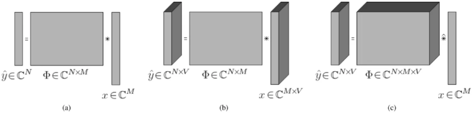
Up to this point, a unicomponent signal has been ex-amined and its classical framework approximation is illustrated in Fig. 1(a). In the multicomponent case, the signal studied be-comes , with denoting the number of components. Two problems can be considered, which depending on the na-tures of and :
• unicomponent and multicompo-nent, the well-known multichannel framework [Fig. 1(b)]; • multicomponent and unicompo-nent, the multivariate framework [Fig. 1(c)], which con-siders as an element-wise product along the dimension
.
The difference between the multichannel and multivariate frameworks is the approximation model, and we will detail this for both frameworks.
Multichannel sparse approximation [28]–[31] is also known as simultaneous sparse approximation (SSA) [32]–[36], sparse approximation for multiple measurement vector (MMV) [37], [38], joint sparsity [39] and multiple sparse approximation [40]. In this framework, all of the components have the same dictio-nary and each component has its own coding coefficient. This means that all components are described by the same profiles
Fig. 1. Decomposition with (a) classical, (b) multichannel, and (c) multivariate frameworks. In (c), is considered as an element-wise product along the dimension .
(atoms), although with different energies: each profile is linearly mixed in the different channels. This framework is also known as a blind source separation problem.
The multivariate framework can be considered as the inverse framework: all of the components have the same coding co-efficient, and thus the multivariate signal is approximated sparsely as the sum of a few multivariate atoms . Data that come from different physical quantities, that have dissimilar characteristic profiles, can be aggregated in the different com-ponents of the multivariate kernels: they must only be homoge-neous in their dimensionalities. To our knowledge, this frame-work has been considered only in [41] for an MP algorithm, although with a particular dictionary template that included a mixing matrix. In the present study, we focus mainly on this multivariate framework, with multivariate and normed (i.e., each multivariate atom is normed, such that ).
In this paragraph, we consider DLAs that deal with multi-component signals. Based on the multichannel framework, the dictionary learning presented in [42] uses a multichannel MP for sparse approximation and the update of K-SVD. We note that the two channels considered are then updated alternatively. In bimodal learning with audio–visual data [16], each modality (audio/video) has its own dictionary and its own coefficient for the approximation, and the two modalities are updated simulta-neously. We also mention [43] based on the multichannel frame-work: they used multiplicative updates for ensuring the nonneg-ativity of parameters.
B. The Shift-Invariant Case
In the shift-invariant case, we want to sparsely code the signal as a sum of a few short structures, known as kernels, that are characterized independently of their positions. This model is usually applied to time series data, and it avoids block effects in the analysis of largely periodic signals and provides a compact kernel dictionary [12], [13].
The shiftable kernels (or generating functions) of the com-pact dictionary are replicated at all of the positions, to pro-vide the atoms (or basis functions) of the dictionary . The samples of the signal , the residue , and the atoms are indexed3by . The kernels can have different lengths.
The kernel is shifted in the samples to generate the atom : zero padding is carried out to have samples. The
3Remark that and do not represent samples, but the signal
and its translation of samples.
subset collects the active translations of the kernel . For the few kernels that generate all of the atoms, (1) becomes
(2)
Due to shift-invariance, is the concatenation of Toeplitz matrices [14], and is times overcomplete. In this case, the dictionary is said convolutional. As a result, in the present study, the multivariate signal is approximated as a weighted sum of a few shiftable multivariate kernels .
Some DLAs are extended to the shift-invariant case. Here all of the active translations of a considered kernel are taken into account during the update step [12]–[15], [44], [45]. Further-more, some of them are modified, to deal with the disturbances introduced by the overlapping of the selected atoms, such as ex-tensions of K-SVD [46], [47] and ILS-DLA (with a shift factor of 1) [48].
C. Remarks on the Multivariate Framework
Usually, the multivariate framework is approached using vec-torized signals. The multicomponent signal is vertically vector-ized from to , and the dictionary from to . After applying the classical OMP, the processing is equivalent to the multivariate one. In this paragraph, we explore the advantages of using the multivariate framework, rather than the classical (unicomponent) one.
In our case, the different components are acquired simulta-neously, and the multivariate framework allows this temporal structure of the acquired data to be keep. Moreover, these com-ponents can be very heterogeneous physical quantities. Vector-izing components causes a loss of physical meaning for sig-nals and for dictionary kernels, and more particularly when the components have dissimilar profiles. We prefer to consider the data studied as being multicomponent: the signals and the dic-tionary have several simultaneous components, as illustrated in the following figures. For the algorithmic implementation, in the shift-invariant case the multivariate framework is easier to im-plement and has a lower complexity than the classical one with vectorized data (see Appendix A).
Moreover, the multivariate framework sheds new light on the topic when multicomponent signals are being processed (see Section IV-B). Furthermore, presented in this way, the
2DRI case is viewed as a simple specification of the multi-variate framework, mostly involving the selection step (see Section VI). The rotation mixes the two components which are acquired simultaneously but which were independent previ-ously, that is easy to see with multivariate signals as opposed to vectorized ones.
Consequently, the multivariate framework is principally in-troduced for the clearness of the explanations and for the ease of algorithmic implementation. Thus, we are going to present multivariate methods that existed under another less-adapted formalism, and were introduced in [49] and [50]: multivariate OMP and multivariate DLA.
IV. MULTIVARIATEORTHOGONALMATCHINGPURSUIT
In the present study, sparse approximation can be achieved by any algorithm that can overcome the high coherence that is due to the shift-invariant case. For real-time applications, OMP is chosen because of its tradeoff between speed and performance [23]. In this section, OMP and M-OMP are explained step by step.
A. OMP Presentation
As introduced in [22], OMP is presented here for the uni-component case and with complex signals. Given a redundant dictionary, OMP produces a sparse approximation of a signal (Algorithm 1). It solves the least squares problem on an iteratively selected subspace.
After initialization (step 1), at the current iteration , OMP selects the atom that produces the absolute strongest decrease in the mean square error (MSE) . This is equivalent to finding the atom that is the most correlated to the residue (see Appendix B). In the shift-invariant case, the inner product between the residue and each atom is now replaced by the correlation with each kernel (step 4), which is generally com-puted by fast Fourier transform. The noncircular complex cor-relation between signals and is given by
(3) The selection (step 6) determinates the optimal atom, charac-terized by its kernel index and its position . An ac-tive dictionary is formed, which collects all of the selected atoms (step 7), and the signal is projected onto this selected subspace. Coding coefficients are computed via the orthog-onal projection of on (step 8). This is carried out recur-sively, by block matrix inversion [22]. The vector obtained, , is reduced to its active (i.e., nonzero) coefficients, denoting by , the trans-pose operator.
Different stopping criteria (step 11) can be used: a threshold on , the number of iterations, a threshold on the relative root MSE (rRMSE) , or a threshold on the decrease in the rRMSE. In the end, the OMP provides a -sparse approxi-mation of
(4) The convergence of OMP is demonstrated in [22], and its recovery properties are analyzed in [23] and [51].
Algorithm 1: 1: initialization: dictionary 2: repeat 3: for do 4: Correlation: 5: end for 6: Selection: 7: Active Dictionary: 8: Active Coefficients: 9: Residue: 10:
11: until stopping criterion
B. Multivariate OMP Presentation
After the necessary OMP review, we now present the M-OMP (Algorithm 2), to handle the multivariate framework described previously (Sections III-A and III-C). The multivariate frame-work is mainly taken into account in the computation of the correlations (step 4) and the selection (step 6). The following notation is introduced: is the th component of the mul-tivariate signal .
For a comparison between the two frameworks from Section III-A, we look at the selection step, with the objective function named as :
(5) In the multichannel framework, selection is based on the inter-channel energy:
(6) with , or [38]. The search for the maximum of the norms applied to the vectors is equivalent to applying a mixed norm to the correlation matrix . This provides a struc-tured sparsity that is similar to the Group-lasso, as explained in [40].
In the multivariate framework that we will consider, the selec-tion is based on the average correlaselec-tion of the components. Using the definition of the inner product given in Section I, we have
(7) In fact, this selection is based on the inner product, which is comparable to the classical OMP, but in the multivariate case. Added to the difference of the approximation models (Section III-A), these two frameworks do not select the same atoms. Due to the absolute values, the noncollinearity or anticollinearity of components are not taken into account in (6), and the multichannel selection is only based on the energy. The multivariate selection (7) is more demanding, and it searches for the optimal tradeoff between components : it keeps the atom that best-fits the residue in each component. The selections are equivalent if all are collinear and in
the same direction. The differences between these two types of selection have also been discussed in [41] and [52].
The active dictionary is also multivariate (step 7). For the orthogonal projection (step 8), the multivariate signal
(respectively, dictionary ) is vertically unfolded along the dimension of the components in a unicompo-nent vector (respectively, matrix ). Then, the orthogonal projection of on is recursively com-puted, as in the unicomponent case, using block matrix inver-sion [22]. For this step, in the multichannel framework coeffi-cients are simply computed via the orthogonal projection of on the active dictionary [31].
At the end of this, the M-OMP provides a multivariate -sparse approximation of . Compared to the OMP, the complexity of the M-OMP is only increased by a factor of , the number of components.
Algorithm 2: 1: initialization: , dictionary 2: repeat 3: for do 4: Correlation: 5: end for 6: Selection : 7: Active Dictionary: 8: Active Coefficients: 9: Residue: 10:
11: until stopping criterion
V. MULTIVARIATEDICTIONARYLEARNINGALGORITHM
In this section, we first provide a global presentation of the Multivariate DLA, and then remarks are given. Added to the multivariate aspect, the novelty of this DLA is to combine shift-invariance and online learning.
A. Algorithm Presentation
For more simplicity, a non-shift-invariant formalism is used in this short introduction, with the atoms dictionary . We have a training set of multivariate signals and the index is added to the variables. In our learning algorithm, named M-DLA (Algorithm 3), each training signal is treated one at a time. This is an online alternation between two steps: a multivariate sparse approximation and a multivariate dictionary update. The multivariate sparse approximation (step 4) is carried out by M-OMP:
s.t. (8)
and the multivariate dictionary update (step 5) is based on max-imum likelihood criterion [6], on the assumption of Gaussian noise
s.t. (9)
This criterion is usually optimized by gradient descent [12]–[14]. To achieve this optimization, we set up a sto-chastic Levenberg–Marquardt second-order gradient descent [53]. This increases the convergence speed, blending together
the stochastic gradient and Gauss–Newton methods. The cur-rent iteration is denoted as . For each multivariate kernel , the update rule is given by (see Appendix B):
(10) with as the indices limited to the temporal support, the adaptive descent step, and the Hessian computed as ex-plained in Appendix C. This step is called LM-update (step 5). There are multiple strategies concerning the adaptive step: the classical choice is made (with . The multivariate framework is taken into account in the dictionary update, with all of the components of the multivariate kernel updated simultaneously. Moreover, the kernels are normalized at the end of each iteration, and their lengths can be modified. Kernels are lengthened if there is some energy in their edges and shortened otherwise.
At the beginning of the algorithm, the kernels initialization (step 1) is based as white Gaussian noise. At the end, different stopping criteria (step 8) can be used: a threshold on the rRMSE computed for the whole of the training set, or a threshold on , the number of iterations. In M-DLA, the M-OMP is stopped by a threshold on the number of iterations. We cannot use rRMSE here, because at the beginning of the learning, the kernels of white noise cannot span a given part of the space studied.
Algorithm 3:
1: initialization: kernels of white noise 2: repeat
3: for do
4: Sparse Approximation:
5: Dictionary Update: -update 6:
7: end for
8: until stopping criterion
B. Remarks About the Learning Processes
In this paragraph, a non-shift-invariant formalism is used for simplicity, with the atom dictionary . We define
as the training set.
The learning algorithms K-SVD [8] and ILS-DLA [18] have
batch alternation: sparse approximation is carried out for the
whole finite training set , and then the dictionary is updated. If the usual convergence of the algorithms is observed empirically, theoretical proof of the strict decrease in the MSE at each iter-ation is not available, due to the nonconvexity of the sparse ap-proximation step carried out using -Pursuit algorithms. Con-vergence properties for dictionary learning are discussed in [54] and [55].
An online (also known as continuous or recursive) alterna-tion can be set up, where each training signal is processed one at a time. The dictionary is updated after the sparse approxi-mation of each signal (so there is more updates than for batch alternation). The processing order of the training signals is often random, so as not to influence the optimization path in a deterministic way. The first-order stochastic gradient descent used in [11] provides a learning algorithm with low memory and computational requirements, with respect to batch algorithms.
Bottou and Bousquet [56] explained that in an iterative process, each step does not need to be minimized perfectly to reach the expected solution. Thus, they proposed the use of stochastic gra-dient methods. Based on this, the faster performances of on-line learning are shown in [57] and [58], for small and large datasets. An online alternation of ILS-DLA, known as recur-sive least-squares DLA (RLS-DLA), is presented in [59], and this also shows better performances. Our learning algorithm is an online alternation, and we can tolerate fluctuations in the MSE. The stochastic nature of the online optimization allows a local minimum to be drawn out. Contrary to the K-SVD and ILS-DLA, we have never observed that the learning gets stuck in a local minimum close to the initial dictionary.
The nonconvex optimization of the M-OMP, the alternating minimization and the stochastic nature of our online algorithm do not allow to ensure the convergence of the M-DLA towards the global minimum. However we find a dictionary, minimum local or global, which assures the decompositions sparsity.
VI. THE2D ROTATIONINVARIANTCASE
Having presented the M-OMP and the M-DLA, these algo-rithms are now simply specified for the 2D rotation invariant case.
A. Method Presentation
To process bivariate real data, we specify the multivariate framework for the bivariate signals. The signal under study,
, is now considered. Equation (2) becomes
(11)
with representing the multivariate concatenation, not the vertical one. This case will be referred to as the oriented case in the following, as bivariate real kernels cannot rotate and are defined in a fixed orientation.
Studying bivariate data, such as 2D movements, we aspire to characterize them independently of their orientations. M-OMP is now specified for this particular 2DRI case. The rotation in-variance implies the introduction of a rotation matrix
of angle for each bivariate real atom . So (11) be-comes
(12) Now, in the selection step (Algorithm 2, step 6), the aim is to find the angle that maximizes the correlations . A naive approach is the sampling of into angles and the addition of a new degree of freedom in the correlations computation (Algorithm 2, step 4). The complexity is increased by a factor of with respect to the M-OMP used in the oriented case. Note that this idea is used for processing bidimensionnal signals such as images [60], although this represents a problem different from ours.
To avoid this additional cost, we transform the signal from to (i.e., , with the imaginary number ). The kernels and coding coefficients are now complex as well.
Retrieving (2), the M-OMP is now applied. For the coding co-efficients, the modulus gives the coefficient amplitude and the argument gives the rotation angle:
(13) Finally, the decomposition of signal is given as
(14)
Now the kernel can be rotated, as here kernels are no longer learned through a particular orientation, as in the previous ap-proach as oriented (M-OMP with and ). Thus, the kernels are shift and rotation invariant, providing a
non-ori-ented decomposition (M-OMP with and ). This 2DRI specification of the sparse approximation
(re-spectively, dictionary learning) algorithm is now denoted as
2DRI-OMP (respectively, 2DRI-DLA). It is important to note that the 2DRI implementations are not different from the algo-rithms presented before; they are just specifications. Only the initial arrangement of the data and the use of the argument of the coding coefficients are different.
B. Notes
In the multisensor case, sensors that acquire bivariate sig-nals are considered. The sensors are physically linked, and so they are under the same rotation. For example, bivariate real signals from a velocity sensor (for velocities and ), an ac-celerometer (for accelerations and ), a gyrometer (for an-gular velocities and ), etc., can be studied. These signals can be aggregated together in such that
(15)
Here, the common rotation angle is jointly chosen between the three complex components due to the multivariate methods. Thus, when used with several complex components, M-OMP (respectively, M-DLA) can be viewed as a joint 2DRI-OMP (respectively, 2DRI-DLA).
We also note that when the number of active atoms , the 2DRI problem considered is similar to 2D curve matching [61]. Schwartz and Sharir provided an analytic solution to com-pute , although their approach is very long, as it is com-puted for each and each . The use of the complex signals indi-cated above allows this problem to be solved nicely and cheaply. Still considering , Vlachos et al. [62] provided rotation invariant signatures for trajectory recognition. However, as with most of methods based on invariant descriptors, their method loses rotation parameters, which is contrary to our approach.
VII. APPLICATIONDATA ANDEXPERIMENTS
After having defined our methods, we present in this section the data that are processed and then the experimental results.
A. Application Data
Our methods are applied to the Character Trajectory motion signals that are available from the University of California at Irvine (UCI) database [63]. They have been initially dealt with
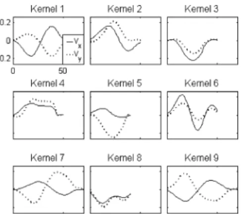
Fig. 2. Non-oriented learned dictionary (NOLD) of the velocities processed by 2DRI-DLA. Each kernel is composed of the real part (solid line) and the imaginary part (dotted line).
a probabilistic model and an expectation-maximization (EM) learning method [64], although without real sparsity in the resulting decompositions. The data comprise 2858 handwritten characters that were acquired with a Wacom tablet sampled at 200 Hz, with about a hundred occurrences of 20 letters written by the same person. The temporal signals are the Cartesian pen-tip velocities and . As the velocity units are not stated in the dataset description, we cannot define this here.
Using the raw data, we aim to learn an adapted dictionary to code the velocity signals sparsely. A partition of the database signals is made, as a training set for applying M-DLA, which is composed of 20 occurrences of each letter ( char-acters), and a test set for qualifying the sparse coding efficiency ( characters). These two sets are used in the following sections.
Although some of the comparisons are made with the oriented case, the results are mainly presented in the non-oriented case. For the differences in data arrangement, we note that in the ori-ented case, the signals are set as , whereas in the non-oriented case they are set as . In these two cases, the dictionary learning algorithms begin their optimiza-tion with kernels initialized on white Gaussian noise.
Three experiments are now detailed, for the dictionary learning, the decompositions on the data, and the decomposi-tions on the revolved data.
B. Experiment 1: Dictionary Learning
In this experiment, the 2DRI-DLA is going to provide a non-oriented learned dictionary (NOLD). The velocities are used to have the kernels as null at their edges. This avoids the introduc-tion of discontinuities in the signal during the sparse approxi-mation.4The kernel dictionary is initialized on white Gaussian
noise, and 2DRI-DLA is applied to the training set. We obtain a velocity kernel dictionary as shown in Fig. 2, where each kernel is composed of the real part (solid line) and the imaginary part (dotted line). This convention for the line style in Fig. 2 will be used henceforth.
The velocity signals are integrated only to provide a more vi-sual representation. However, due to the integration, the two dif-ferent velocities kernels provide very similar trajectories (inte-grated kernels). The inte(inte-grated kernel dictionary (Fig. 3) shows
4Note also that contrary to the position signals, the velocity signals allow
spatial invariance (different from the temporal shift-invariance).
Fig. 3. Rotatable trajectory dictionary associated to the non-oriented learned dictionary (NOLD) processed by 2DRI-DLA.
Fig. 4. Utilization matrix of the dictionary computed on the learning set. The means of the coefficient absolute values are given as a function of the kernel indices and the letters.
that motion primitives are successfully extracted by the 2DRI-DLA. Indeed, the straight and curved strokes shown in Fig. 3 correspond to the elementary patterns of the set of handwritten signals.
The question is how to choose the dictionary size hyperpa-rameter . In the non-oriented case, 9 kernels are used, whereas in the oriented case, 12 are required. The choice is an empir-ical tradeoff between the final rRMSE obtained on the training set, the sparsity of the dictionary, and the interpretability of the resulting dictionary (criteria that depend on the application can also be considered).
As interpretability is a subjective criterion, a utilization ma-trix is used in supervised cases (Fig. 4). The mean of the co-efficients absolute values (gray shading level) computed on the learning set is mapped as a function of the kernel index (or-dinate), with the signal class as a letter (abscissa). The letters are organized according to the similarities of their utilization profiles. We can say that a dictionary has a good interpretability when well-used kernels are common to different letters that have related shapes (intuitively, other tools can be imagined to define a dictionary). For example, letters and have some similar-ities and share kernel 7. Similarly, and share kernel 9.
We also note here that during M-DLA, M-OMP provides a -sparse approximation (Section V-A). is the number of ac-tive coefficients, and it determinates the number of underlying primitives (atoms) that are searched and then learned from each
Fig. 5. Original (a) and reconstructed (b) velocity signals of five occurrences of the letter (real part, solid line; imaginary part, dotted line), and their associated spikegram (c).
signal. If the dictionary size is too small compared to the ideal total number of primitives we are searching, the kernels will not be characteristic of any particular shape and the rRMSE will be high. Conversely, if and are particularly important, the dictionary learning will tend to scatter the information into the plentiful kernels. Here, the utilization matrix will be very smooth, without any kernel characteristics for particular letters. If is particularly important and is optimal, we can see that some kernels will be characteristic and well used, while others will not be. The utilization matrix rows of unused kernels are white, and it is easy to prune these to obtain the optimal dic-tionary. Typically, in our dictionary, kernel 8 can obviously be pruned (Fig. 4). Therefore, it is preferable to slightly overesti-mate .
Finally, the crucial question is how to choose the parameter . Indeed, this choice is empirical, as it depends on the number of primitives that the user forecasts to be in each signal of the dataset studied. In our experiment, we choose , as 2–3 primary primitives coding the main information, and the re-maining ones coding the variabilities.
The nonconvex optimization of the M-OMP and the random processing of the training signals induce different dictionaries that are obtained with the same parameters. However, the vari-ance of the results is small, and sometimes we obtain exactly the same dictionaries, or they have similar qualities (rRMSE, dictio-nary size, interpretability). For the following experiments, note that an oriented learned dictionary (OLD) is also processed by M-DLA.
C. Experiment 2: Decompositions on the Data
To evaluate the sparse coding qualities, non-oriented decom-positions of five occurrences of the letter on the NOLD are considered in Fig. 5. The velocities [Fig. 5(a)] [respectively, Fig. 5(b)] are the original (respectively, reconstructed, i.e., approximated) signals, which are composed of the real part (solid line) and the imaginary part (dotted line). The rRMSE on the velocities is around 12%, with 4–5 atoms used for the
Fig. 6. Letter (respectively, ). Original (a) [respectively, (d)], oriented re-constructed (b) [respectively, (e)], and non-oriented rere-constructed (c) [respec-tively, (f)] trajectories.
reconstruction (i.e., approximation). The coding coefficients are illustrated using a time-kernel representation [Fig. 5(c)] called spikegram [13]. This provides the four variables:
1) the temporal position (abscissa); 2) the kernel index (ordinate);
3) the coefficient amplitude (gray shading level); 4) the rotation angle (number next to each spike, in
de-grees).
The low number of atoms used for the signal reconstruc-tion shows the decomposireconstruc-tion sparsity, which we refer to as the
sparse code. The primary atoms are the largest amplitude ones,
like kernels 2, 4, and 9, and these concentrate the relevant in-formation. The secondary atoms code the variabilities between different realizations. The reproducibility of the decompositions is highlighted by the primary-atom repetition (amplitudes and angles) of the different occurrences. The sparsity and repro-ducibility are the proof of an adapted dictionary. Note that the spikegram is the result of the signal deconvolution through the learned dictionary.
The trajectory of the original letter [Fig. 6(a)] [respectively, , Fig. 6(d)] is reconstructed with the primary atoms. We com-pare the oriented case [Fig. 6(b)] [respectively, Fig. 6(e)] using the OLD and the non-oriented case [Fig. 6(c)] [respectively, Fig. 6(f)] using the NOLD. For instance, for the reconstruction, the letter [Fig. 6(c)] is rebuilt as the sum of the NOLD kernels 2, 4, and 9 (the shapes can be seen in Fig. 3), which are specified by the amplitudes and the angles of the spikegram (Fig. 5(c)). We now focus on the principal vertical stroke that is common to letters and [Fig. 6(a) and (d)]. To code this, the oriented case uses two different kernels: kernel 5 for [Fig. 6(b), dotted line] and kernel 12 for [Fig. 6(e), dashed line]. However, the non-oriented case needs only one kernel for these two letters: kernel 9 [Fig. 6(c) and (f), solid line], which is used with an av-erage rotation of 180 . Thus, the non-oriented approach reduces
Fig. 7. Velocity signals revolved by 45 (a) [respectively, 90 (d)] and reconstructed (b) [respectively, (e)] for two occurrences of the letter , and their associated spikegram (c) [respectively, (f)].
Fig. 8. Trajectory of letter revolved by (a) an angle of 90 , and (b) the oriented reconstructed and (c) the non-oriented reconstructed.
the dictionary redundancy and provides an even more compact rotatable kernel dictionary. The detection of rotational invari-ants allows the dictionary size to decrease from 12 for the OLD, to 9 for the NOLD.
D. Experiment 3: Decompositions on Revolved Data
To simulate the rotation of the acquiring tablet, we artifi-cially revolved the data of the test set, with the characters now rotated by angles of 45 and 90 (with the previous dic-tionaries kept). Fig. 7 shows the non-oriented decompositions of the second and third occurrences of the examples used in Fig. 5. The velocity signals rotated by 45 [Fig. 7(a)] [respec-tively, 90 , Fig. 7(d)] are reconstructed in a non-oriented ap-proach [Fig. 7(b)] [respectively, Fig. 7(e)]. In these two cases, the rRMSE is identical to the previous experiment, when the characters were not revolved. Fig. 7(c) [respectively, Fig. 7(f)] shows the associated spikegrams. The angle differences of the primary kernels between the spikegrams [Figs. 5(c), 7(c), and (f)] correspond to the angular perturbation we applied. This shows the rotation invariance of the decomposition.
The trajectory of letter revolved by 90 [Fig. 8(a)] is reconstructed with the primary kernels, with a comparison of the oriented case [Fig. 8(b)] using the OLD, and the non-ori-ented case [Fig. 8(c)] using the NOLD. In the orinon-ori-ented case, the rRMSE increases from 15% [Fig. 6(b)] to 30% [Fig. 8(b)], and the sparse coding is less efficient. Moreover, the selected kernels
Fig. 9. Reconstruction rate on the test set as a function of the sparsity of the approximation for the different dictionaries.
are different, with there being no more reproducibility. The dif-ference between these two reconstructions shows the necessity to be robust to rotations. In the non-oriented case, the rRMSE is equal to whatever the rotation angle is [Figs. 6(c) and 8(c)], and it is always less than the oriented case. The selected kernels are identical in the two cases, and they show the rotation invariance of the decomposition.
To conclude this section, the methods have been validated on bivariate signals and have shown rotation invariant sparse coding.
VIII. COMPARISONS
Three comparisons are made in this section: the dictionaries learned by our algorithms are first compared to classical dictio-naries, then they are compared together, and finally the M-DLA is compared to the other dictionary learning algorithms.
A. Comparison With Classical Dictionaries
In this section, the test set is used for the comparison, although the characters are not rotated any more, and only com-ponent is considered (to be in the real unicomponent case). We compare the previous learned dictionaries for the non-ori-ented approach (the NOLD, with ) and the oriented approach (the OLD, with ) to the classical dictionaries based on fast transforms, including: discrete Fourier transform (DFT), discrete cosine transform (DCT), and biorthogonal wavelet transform (BWT) (different types of wavelets that give similar performances; we only present the CDF 9/7). For each dictionary, -sparse approximations are computed on the test set, and the reconstruction rate is then computed. This is defined as:
(16)
The rate is represented as a function of in Fig. 9.
We see that for a very few coefficients, the signals are re-constructed better with learned dictionaries (NOLD and OLD ) than with Fourier based dictionaries (DFT and
TABLE I
RECONSTRUCTIONRATERESULTS ON THETESTSET
Fig. 10. Utilization matrix for the OLD on set . The means of the absolute values of the coefficients is given as a function of the kernel indices and the letters. The letters with are those that are revolved.
DCT), which are themselves better than5wavelets (BWT). The
results show the optimality of learned dictionaries over generic ones. If the dictionary learning is long compared to fast trans-forms, it is computed a single time for a given application. For the NOLD, only 7 atoms are needed to reach a rate of 90%, and the asymptote is at 93%. Furthermore, what-ever . Rotation invariance is thus useful even without data rotation, as it provides a better fit of the variabilities between the different realizations.
Rates beyond are not represented in Fig. 9, although the classical dictionaries can be seen to reach a reconstruction rate of 100%; they span all of the space, in contrast to learned dictionaries. This is because generic dictionaries are bases of the
space, whereas learned dictionaries can be considered as a sort
of bases of the studied phenomenon. In DLAs, the sparse ap-proximation algorithm selects strong energy patterns, and these are then learned. So all of the signal parts that are never selected are never learned, which generally means the noise, although not always.
B. Comparison Between Oriented and Non-Oriented Learning
In Section VII-D, we only evaluated the rotation invariance of the decompositions with rotated data, and not the rotation invariance of the learning. The data in the test set were revolved, but not the data of the learning set. Here, we propose to study the rotation invariance of the whole learning method with rotated training signals.
5Note that this is due to the piecewise sinus aspect of the signals studied. This
confirms that DCT appears to be the more adapted to motion data [65].
TABLE II
SIMILARITYCRITERIONRESULTS ON THETESTSET
In this comparison, learning and decompositions are carried out on datasets (including the training set and the test set), which are revolved at different angles. contains the original data, contains the original data and the data revolved by 120
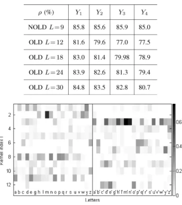
contains the original data and the data revolved by 120 and 240 , and contains the original data and the data revolved by random angles. The training sets allow the learning of different dictionaries: the NOLD with 9 kernels and the OLD with 12, 18, 24, and 30 kernels. The decompositions on the test sets give the reconstruction rates , with .
Table I gives the results of the reconstruction rates according to the datasets (columns) and the dictionary type (rows). For the non-oriented learning, the results are similar, whatever the dataset. For oriented learnings, the approximation quality in-creases with the kernel number. The extra kernels can span the space better. However, even with 30 kernels, the OLD shows re-sults worse than the NOLD with only 9 kernels. Moreover, the reconstruction rate decreases when number of different angles in the dataset increases, with revolved letters are considered as new letters.
These results only allow the approximation quality to be seen, and not the rotation invariance and the reproducibility of the decompositions. So, a similarity criterion is going to be set up, using the utilization matrix. As explained in Section VII-B, this matrix is formed by computing the means of coefficients abso-lute values of the test-set decompositions. As seen in Fig. 10, the values are given as a function of the kernel indices (ordinate) and the letters (abscissa). Fig. 10 shows the utilization matrix computed on for the OLD, with . It can be seen that it is not the same kernels that are used to code a letter and its ro-tation, denoted by . To evaluate this phenomenon, the simi-larity criterion is defined as the mean of the normalized scalar products between the column of a letter and that of its rotation. Table II summarizes the mean scalar product given in the percentage according to the datasets (columns) and the dictio-nary type (rows). The criterion definition and the test-set de-sign were chosen to give 100% in the reference non-ori-ented case. This remains at 100% whatever the dataset, which shows the rotation invariance. However, in reality, it is no use to carry out learning on the rotated data. As seen in Section VII-D, non-oriented learning on the original data is sufficient for an adapted dictionary that is robust to rotations.
For the oriented learnings, although bigger dictionaries give better reconstruction rates (Table I), they have poorer similarity criteria, as multiple kernels tend to scatter the information.
Therefore, artificially increasing the dictionary size is not a good idea for sparse coding, because it damages the results. Furthermore, increasing the number of different angles in the dataset gives better reproducibility, as the signals no longer influence the learning through a fixed orientation, and conse-quently the oriented kernels are the more general.
C. Comparison With Other Dictionary Learning Algorithms
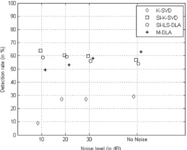
We now compare our method to other DLAs. The advantages of online learning have already been pointed out in [11], [57], [58], so our experiment is on the robustness to shift-invariance. M-DLA is used in real and unicomponent cases, to compare it with the existing learning methods: K-SVD [8], the shift-in-variant version of K-SVD [46] known as SI-K-SVD, and the shift-invariant ILS-DLA [48] (the shift factor is set as up to 1), which is indicated as SI-ILS-DLA in the following.
This comparison is based on the experience described in [46]. A dictionary of kernels is created randomly and the kernel length is 18 samples. The training set is composed of 2000 signals of length 20, and it is synthetically gen-erated from this dictionary. For the kernels, circular shifts are not allowed, and so only three shifts are possible. Each training signal is composed of the sum of three atoms, for which the amplitudes, kernels indices and shift parameters are randomly drawn. White Gaussian noise is also added at several levels: an SNR of 10, 20, and 30 dB, and without noise. All of the learning algorithms are applied with the same parameters, with the dic-tionary initialization made on the training set, and the sparse approximation step carried out by OMP. The learned dictionary is returned after 80 iterations. Classical K-SVD is also tested, with hopes of recovering an atoms dictionary of 135 atoms (the 45 kernels in the three possible shifts).
In the experiment, a learned kernel is considered as detected, i.e., recovered, if its inner product with its corresponding original kernel is such that
(17) The high threshold of 0.99 was chosen by [46]. For each learning algorithm, the detection rate of the kernels is plotted as a function of the noise level, which was averaged over five tests (Fig. 11).
This experiment only tests the algorithm precision. In our case, the online alternation provides learning that is fast, but not so precise, due to the stochastic noise that is induced by the random choice of a training signal at each iteration. We observe that 80% of the are between 0.97 and 1.00, with only a few above the severe threshold of 0.99. To be comparable with batch algorithms, which are more precise at each step, the clas-sical strategy for the adaptive step proposed in Section V-A is adapted to the constraints of this experiment. With 2000 training signals, we prefer to keep a constant step for one loop of the training set. Moreover, the step is increased faster, to provide satisfactory convergence after 80 iterations. For the first 40 it-erations, the step is set up as: , and then it is kept constant for the last iterations: . The results obtained are now plotted in Fig. 11.
Fig. 11 shows that having a shift-invariant model is obviously relevant. For shift-invariant DLAs, this underlines their ability to recover the underlying shift-invariant features. However, we observe that the M-DLA performance decreases when the noise
Fig. 11. Detection rate as a function of noise level for K-SVD (diamonds), SI-K-SVD (squares), SI-ILS-DLA (circles) and M-DLA (stars).
levels increase, contrary to SI-K-SVD and SI-ILS-DLA, which appear not to be influenced in this way. Despite its stochastic up-date, our algorithm recovers the original dictionary in a similar proportion to the batch algorithms. This experiment supports the analysis of [56] relating to learning, where each step does not need to be minimized exactly to converge towards the expected solution.
IX. DISCUSSION
Dictionary learning allows signal primitives to be recovered. The resulting dictionary can be thought of as a catalog of el-ementary patterns that are dedicated to the application consid-ered and that have a physical meaning, as opposed to classical dictionaries such as wavelets, curvelets, etc. Therefore, decom-positions based on such a dictionary are made sparsely on the underlying features of the signal set studied. For the rRMSE, the few atoms used in the decompositions shows the efficiency of this sparse-coding method.
The non-oriented approach for sparse coding reduces the dic-tionary size in two ways:
1) when the signals studied cannot rotate, the non-oriented ap-proach detects rotational invariants (the vertical strokes of letters and , for example), which reduces the dictionary size;
2) when the signals studied can rotate. To provide efficient sparse coding, the oriented approach needs to learn motion primitives for each of the possible angles. Conversely, in the non-oriented case, single learning is sufficient. This provides a noticeable reduction of the dictionary size. In this way, the shift-invariant and rotation invariant cases provide a compact learned dictionary . Moreover, the non-oriented approach allows robustness for any writing direc-tion (tablet rotadirec-tion) and for any writing inclinadirec-tion (intra- and inter-user variabilities). When added to a classification step, the angles information allows the orientation of the writing baseline to be given.
Recently, Mallat notes [66] that the key for the classifica-tion is not the representaclassifica-tion sparsity but its invariances. In our 2DRI case, the decompositions are invariant to temporal
shift (parameter ), to rotation (parameter ), to scale (param-eter ) and to spatial translation (use of velocity signals in-stead of position signals). Based on these considerations, we are also working on the classification of sparse codes, to carry out gesture recognition, and the first experiments look promising. Spikegrams appear to be good representations for classification, and their reproducibility can be exploited. The classification re-sults are interesting, because kernels are learned only with data-fitting criterion of unsupervised dictionary learning, and so without discriminative constraints. It appears that recovering the primitives underlying the features of a signal set via a sparsity constraint allows this set to be described discriminatively.
Motion data is new with regards to custom sparse coding applications. Recently, we have taken cognizance of a work made on multicomponent motion signals. In [67], Kim et al. use a tensor factorization with tensor constraints to make a multicomponent dictionary learning. Modelized by the multi-variate framework and processed by our proposed algorithms, this problem is solved without the heavy tensor formalism.
X. CONCLUSION
In contrast to the well-known multichannel framework, a multivariate framework was introduced to more easily present our methods relating to bivariate signals. First, the multivariate sparse-coding methods were presented: Multivariate OMP, which provides sparse approximations for multivariate sig-nals, and Multivariate DLA, which is a learning algorithm that empirically learns the optimal dictionary associated to a multivariate signal set. All of the dictionary components are updated simultaneously. The resulting dictionary jointly provides sparse approximations of all of the signals of the set considered. This DLA is an online alternation between a sparse approximation step carried out by M-OMP, and a dictionary update that is optimized by stochastic Levenberg–Marquardt second-order gradient descent. The online learning does not disturb the performance of the dictionary obtained, even in the shift-invariant case.
Then in dealing with bivariate signals, we wanted the de-compositions to be independent of the orientation of the move-ment execution in 2D space. To provide rotation invariant sparse coding, the methods were simply specified to the 2D rotation invariant case, known as 2DRI-OMP and 2DRI-DLA. Rotation invariance is useful, but not only when the data are rotated, as it allows to code variabilities. Moreover, shift-invariant and ro-tation invariant cases induce a compact learned dictionary and are useful for classification. As validation, these methods were applied to 2D handwritten data.
The methods applications are dimensionality reduction, de-noising, gesture representation and analysis, and all of the other processing that is based on multivariate feature extraction. The prospects under consideration are to extend these methods to 3D rotation invariance for trivariate signals, and to present the classification step that is applied to the spikegrams and the as-sociated results.
APPENDIXA
CONSIDERATIONS FOR THEIMPLEMENTATION
We are going to look at the OMP complexity for the dif-ferent approaches in the shift-invariant case. Often enough, the
acquired signals are dyadic (i.e., the signal size is a power of 2). If they are not, they are lengthened by zero-padding to samples, with as the first power of 2 to the . So, in the unicomponent case, the correlation is computed by FFT in for each kernel. In the multivariate case, the multivariate correlation is the sum of the component correla-tions, and it is computed in for each kernel. To retrieve the classical case, we can simply vectorize the signal from to . However, zero-padding be-tween the components is necessary, otherwise the kernel compo-nents can overlap two consecutive signal compocompo-nents during the correlation. Limiting the kernels length to samples (which is a loss of flexibility) with the size of the longest kernel, zero-padding of samples has to be carried out between two consecutive components.
This zero-padded signal of samples is lengthened again, in order to be dyadic. Finally, the correlation complexity
is for each kernel.
Moreover, for the selection step, investigations need to be lim-ited to the first samples of the correlation obtained. To conclude, the multivariate framework is easier to implement and has lower complexity than the classical framework with vector-ized data.
APPENDIXB
COMPLEXGRADIENTOPERATOR
The gradient operator was introduced by Brandwood in [68]. Assuming , the complex derivation rules are
and
[68] showed that the direction of maximum rate of change of an objective function with is
1) The derivation of with respect to
Thus: . This gives the selection step of the OMP (algorithm 1).
2) The derivation of with respect to
Thus: . This gives the first-order part of the update of the M-DLA. The complex least mean squares (CLMS) obtained by the pseudo-gradient [69] is retrieved (give or take a factor of 2). For the complex Hessian, we make reference to [70].
In the shift-invariant case, all of the translations of a consid-ered kernel are taken into account in the dictionary update: , with the error localized at and restrained to the temporal support (i.e., ). This gives the shift-invariant update of the M-DLA (10).
APPENDIXC
CALCULUS OF THEHESSIAN
In this Appendix, we explain the calculation of the Hessian . This allows the adaptive step to be specified to each kernel , and the convergence of the well-used kernels to be stabilized at the beginning of the learning.
An average Hessian is computed for each kernel , not for each sample, to avoid fluctuations between neighboring sam-ples. is thus reduced to a scalar. Assuming the hypothesis of sparsity (a few atoms are used for the approximation), the overlap of selected atoms is initially considered as nonexistent. So the cross-derivative terms of are null, and we have
(18)
For overlapping atoms, the learning method can become un-balanced, due to the error in the gradient estimation. We over-estimate the Hessian slightly to compensate for this. All
are sorted and then indexed by , such that: , with as the cardinal of the set . Denoting as the length of the kernel at the iteration , the set is defined as:
. This allows for the identification of overlap situations. The cross-derivative terms of are no longer con-sidered to be null, and their contributions are proportional to . Double-overlap situations are not considered, when . Due to the hypothesis of sparsity, these situations are considered to be very rare (as is verified in practice), and they are compensated for by overestimating . The absolute value of the cross terms is taken: . The absolute value is not disturbing, even without double overlap, as it is better to slightly overestimate than to underestimate it (it would better move a little but surely). Finally, we propose for the following approximation quickly computed:
(19)
The following comments can be made regarding (19):
• if the gap between two atoms is always greater than , the first approximation of (18) is recovered;
• when the overlap is weak, the cross-products have little influence on the Hessian;
• intra-kernel overlaps have been considered, but not inter-kernel ones. However, we see that inter-inter-kernel overlaps do not disturb the learning, so we ignore their influence. The update step based on (10) and (19) is called LM-update (step 5, Algorithm 3).
Without the Hessian in (10), a first-order update is retrieved. In this case, the convergence speed of a kernel is directly linked to the sum of its decomposition coefficients. Advantage of the Hessian is to tend to make the convergence speed similar for all kernels, independently of their uses in the decompositions. Con-cerning the approximation of the Hessian, at the beginning of the learning, kernels which are still white noises overlap frequently and method can become unbalanced. Increasing the Hessian, the approximation thus stabilizes the beginning of the learning process. After, since kernels converge, overlaps are quite rare and the approximation of the Hessian is closed to (18).
ACKNOWLEDGMENT
The authors would like to thank Z. Kowalski, A. Hanssen, and anonymous reviewers for their fruitful comments, and C. Berrie for his help about English usage.
REFERENCES
[1] A. Bruckstein, D. Donoho, and M. Elad, “From sparse solutions of systems of equations to sparse modeling of signals and images,” SIAM Rev., vol. 51, pp. 34–81, 2009.
[2] S. Mallat, A Wavelet Tour of Signal Processing, 3rd ed. New York: Academic, 2009.
[3] E. Candès and D. Donoho, “Curvelets—A surprisingly effective non-adaptive representation for objects with edges,” in Curves and Sur-faces. Nashville, TN: Vanderbilt Univ. Press, 2000, pp. 105–120. [4] S. Chen, D. Donoho, and M. Saunders, “Atomic decomposition by
basis pursuit,” SIAM J. Sci. Comput., vol. 20, pp. 33–61, 1998. [5] J. Starck, M. Elad, and D. Donoho, “Redundant multiscale transforms
and their application for morphological component analysis,” Adv. Imag. Electron Phys., vol. 132, pp. 287–348, 2004.
[6] B. Olshausen and D. Field, “Sparse coding with an overcomplete basis set: A strategy employed by V1?,” Vision Res., vol. 37, pp. 3311–3325, 1997.
[7] K. Kreutz-Delgado, J. Murray, B. Rao, K. Engan, T. Lee, and T. Se-jnowski, “Dictionary learning algorithms for sparse representation,” Neural Comput., vol. 15, pp. 349–396, 2003.
[8] M. Aharon, M. Elad, and A. Bruckstein, “K-SVD: An algorithm for designing overcomplete dictionaries for sparse representation,” IEEE Trans. Signal Process., vol. 54, no. 11, pp. 4311–4322, 2006. [9] M. Elad and M. Aharon, “Image denoising via sparse and
redun-dant representations over learned dictionaries,” IEEE Trans. Image Process., vol. 15, no. 12, pp. 3736–3745, 2006.
[10] J. Mairal, M. Elad, and G. Sapiro, “Sparse representation for color image restoration,” IEEE Trans. Image Process., vol. 17, no. 1, pp. 53–69, 2008.
[11] M. Aharon and M. Elad, “Sparse and redundant modeling of image content using an image-signature-dictionary,” SIAM J. Imag. Sci., vol. 1, pp. 228–247, 2008.
[12] M. Lewicki and T. Sejnowski, “Coding time-varying signals using sparse, shift-invariant representations,” in Proc. Conf. Adv. Neural Inf. Process. Syst. II, 1999, vol. 11, pp. 730–736.
[13] E. Smith and M. Lewicki, “Efficient coding of time-relative structure using spikes,” Neural Comput., vol. 17, pp. 19–45, 2005.
[14] T. Blumensath and M. Davies, “Sparse and shift-invariant representa-tions of music,” IEEE Trans. Audio, Speech, Lang. Process., vol. 14, no. 1, pp. 50–57, 2006.
[15] B. Olshausen, “Sparse codes and spikes,” in Probabilistic Models of the Brain: Perception and Neural Function. Cambridge, MA: MIT Press, 2001, pp. 257–272.
[16] G. Monaci, P. Vandergheynst, and F. Sommer, “Learning bimodal structure in audio-visual data,” IEEE Trans. Neural Netw., vol. 20, no. 12, pp. 1898–1910, 2009.
[17] K. Engan, S. Aase, and J. Husøy, “Multi-frame compression: Theory and design,” Signal Process., vol. 80, pp. 2121–2140, 2000. [18] K. Engan, K. Skretting, and J. Husøy, “Family of iterative LS-based
dictionary learning algorithms, ILS-DLA, for sparse signal representa-tion,” Digit. Signal Process., vol. 17, pp. 32–49, 2007.
[19] G. Davis, “Adaptive Nonlinear Approximations,” Ph.D. dissertation, New York Univ., New York, 1994.
[20] J. Tropp and S. Wright, “Computational methods for sparse solution of linear inverse problems,” Proc. IEEE, vol. 98, pp. 948–958, 2010. [21] S. Mallat and Z. Zhang, “Matching pursuits with time-frequency
dictio-naries,” IEEE Trans. Signal Process., vol. 41, no. 12, pp. 3397–3415, 1993.
[22] Y. Pati, R. Rezaiifar, and P. Krishnaprasad, “Orthogonal matching pur-suit: Recursive function approximation with applications to wavelet decomposition,” in Proc. Asilomar Conf. Signals, Syst., Comput., Pa-cific Grove, CA, 1993, vol. 1, pp. 40–44.
[23] J. Tropp, “Greed is good: Algorithmic results for sparse approxima-tion,” IEEE Trans. Inf. Theory, vol. 50, no. 10, pp. 2231–2242, 2004. [24] M. Osborne, B. Presnell, and B. Turlach, “A new approach to variable
selection in least squares problems,” IMA J. Numer. Anal., vol. 20, pp. 389–404, 2000.
[25] I. Daubechies, M. Defrise, and C. De Mol, “An iterative algorithm for linear inverse problems with a sparsity constraint,” Commun. Pure Appl. Math., vol. LVII, pp. 1413–1457, 2004.