HAL Id: hal-01761329
https://hal.archives-ouvertes.fr/hal-01761329
Submitted on 9 Apr 2018
HAL is a multi-disciplinary open access
archive for the deposit and dissemination of
sci-entific research documents, whether they are
pub-lished or not. The documents may come from
teaching and research institutions in France or
abroad, or from public or private research centers.
L’archive ouverte pluridisciplinaire HAL, est
destinée au dépôt et à la diffusion de documents
scientifiques de niveau recherche, publiés ou non,
émanant des établissements d’enseignement et de
recherche français ou étrangers, des laboratoires
publics ou privés.
Distributed under a Creative Commons Attribution| 4.0 International License
of Large Amplitude Intramolecular Motion
Guillaume Reinisch, Kenji Miki, G. Vignoles, Bryan Wong, Chris Simmons
To cite this version:
Guillaume Reinisch, Kenji Miki, G. Vignoles, Bryan Wong, Chris Simmons. An Efficient and Accurate
Formalism for the Treatment of Large Amplitude Intramolecular Motion. Journal of Chemical Theory
and Computation, American Chemical Society, 2012, 8, pp.2713 - 2724. �10.1021/ct300278x�.
�hal-01761329�
intramolecular motion.
G. Reinisch, K. Miki, G. L. Vignoles, B. M. Wong
We propose a general approach to describe Large Am-plitude Motions (LAM) with multiple Degrees Of Free-dom (DOF) in molecules or reaction intermediates, which is useful for the computation of thermochemical or ki-netic data. The kiki-netic part of the LAM Lagrangian is derived using a Z-matrix internal coordinate representa-tion within a new numerical procedure. This derivarepresenta-tion is exact for a classical system, and the uncertainties on the prediction of observable quantities largely arise from un-certainties on the LAM Potential Energy Surface (PES). In order to rigorously account for these uncertainties, we present an approach based on Bayesian theory to infer a parametrized physical model of the PES using ab initio calculations. This framework allows a quantification of uncertainties associated with a PES model, as well as a propagation scheme for the final quantity of interest. A selection and generalization of some treatments account-ing for the couplaccount-ing of the LAM with other internal or external degrees of freedom are also presented. Finally, we discuss and validate the approach with two applica-tions: the calculation of the partition function of the 1,3-butadiene, and the calculation of the high-pressure reaction rate of the CH3+ H → CH4recombination.
I. INTRODUCTION
Quantum chemical methods, as implemented in many software packages1,2, nowadays allow for routine
calcu-lations of various properties of molecules. Among them, thermodynamic and kinetic data are crucial for the un-derstanding and prediction of chemical processes3.
A reliable prediction of such properties requires tack-ling two main issues. First, it is necessary to calculate accurate molecular energies at least for some specific ge-ometries defining the energetic minima (stable states) and saddle points (Transition States, TS) on the Po-tential Energy Surface (PES). Modern ab-initio meth-ods are well-adapted and efficient in addressing these issues. A second issue arises when one wishes to com-pute temperature-dependent properties (entropies, heat capacities, reaction rates) for which Densities Of States (DOS) and/or partition functions need to be computed. This is usually achieved using the simple Rigid Rotor Harmonic Oscillator (RRHO) approximation. Indeed, most of the internal vibrations are of small amplitude and are very well described under this approximation. How-ever, it has been shown long ago that these approxima-tions fail when large amplitude moapproxima-tions are involved4,5,
and a rigorous treatment is often required if an accu-rate prediction of statistical properties is required6–8.
This is particularly the case when a torsional motion is
present7,9–11 or when a loose transition state is involved
in a dissociation/recombination reaction12–14. Numerous
studies have been dedicated to the development of sta-tistical methods in the context of one or the other appli-cation, while, to our knowledge, none has been presented for the general case. In cases of torsional motions, the proposed treatments are usually derived from the one-dimensional hindered rotor (1DHR) model, originally proposed by Pitzer et.al.4. Recent studies7,9,11show the
importance of a rigorous treatment, where quantum ef-fects, mutidimensionality, as well as coupling with other internal or external motions, can have a non-negligible influence. In the context of dissociation reactions involv-ing a loose complex, 2- to 5-dimensional large amplitude motions need to be described. Analytical expressions for the kinetic energy of two rigid counterparts have already been derived in previous work12,13,15, and it has been
shown that this formalism gives a very good approxi-mation of the reaction rate, as long as the used PES is determined with a high level of accuracy12,16,17.
Since the kinetic energy operator has an analytic form, the main and most critical issue involved in studies of large amplitude motion is the determination of the PES18,19. Even though first principle calculations have
proven their ability to yield accurate electronic ener-gies, their computational cost does not generally allow for on-the-fly calculations20and, therefore, an
appropri-ate interpolation method has to be used20,21. Three
ap-proaches can be distinguished: (i) local (or weighted) interpolation19,22–24, (ii) global (or non-weighted)
in-terpolation by a set of mathematical functions16,25,26,
and (iii) global interpolation by a parametrized phys-ical model27–30. The first two solutions are general in
principle but tedious to set up in practice when the di-mension of the problem increases. The practical issues involved, along with the large amount of ab initio energy computations required, are important limitations to their utilization. The third solution is a global interpolation by a parametrized physical model of the interaction energy, and is widely referred to as a ’force field’. This particular formalism is extensively used to study the dynamics of large atomic systems31–33. Explicit introduction of the physical contributions to the interaction energy allows for a considerable decrease in the amount of informa-tion required to set up the model. However, because this simplification can introduce large model errors, it is of primary importance to estimate the confidence expected on a final Quantity of Interest (QoI). Only very recently has this issue been addressed by Cailliez and Pernot34.
By using a Bayesian approach, they have calculated the parameter uncertainties associated with a Van der Waals type PES, and have evaluated their influence on the un-, C. Simmons
certainties for the thermodynamic data. A major conclu-sion of their work is that the PES model error is indeed a critical feature when one wants to predict thermody-namic properties.
The purpose of this paper is twofold. First, we present a general procedure based on a Bayesian framework to in-fer a system-specific force field. This procedure allows the computation of Probability Density Functions (PDFs) of the model parameters using a set of ab initio data, and also allows their propagatation to the desired QoI (here, partition function or reaction rate). The other concern of this paper is the presentation of a general approach for characterizing the statistical properties of an LAM. The restriction of previous methods to specific types of motion, largely due to an ad hoc derivation of the ki-netic energy of the system, is overcome by introducing a new numerical method based on a functional Z-Matrix, in which the Degrees Of Freedom (DOFs) are written as functions of generalized coordinates. This approach pro-vides several advantages: (i) the dynamical variables can be of any kind (bond length, bending or dihedral angle, reaction path-like coordinate, etc.), (ii) the geometry re-laxation as well as the constraints are easily expressed in the Z-Matrix formalism, and (iii) the numerical imple-mentation is straightforward and robust. Other issues, such as quantum effects and couplings between LAMs with the overall rotation and the internal HO, are ap-proximately taken into account using selected methods from the literature7,11.
To illustrate the advantages and accuracies of the pro-posed methodology, two calculation tests are presented: (i) the partition function of 1,3-butadiene, and (ii) the high-pressure limit of the CH3+H→ CH4reaction rate.
The presented methods are part of the currently devel-oped C++ library openSOAMS35.
II. THEORY
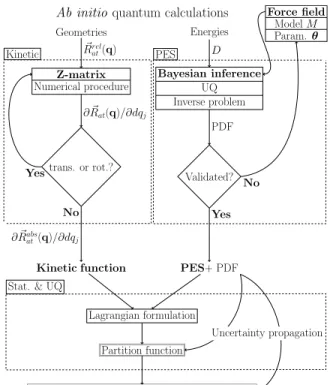
The overall methodology proposed in this paper is il-lustrated in figure 1. The particular steps which are emphasized in this work are (i) the inference of a PES model (parametrized by the vector θ) from a set of ab initio energies (’PES’ box), (ii) the implementation of a Z-matrix coordinate system for the computation of the kinetic function (’Kinetic’ box) , and (iii) the Lagrangian analysis of the LAM and PES uncertainty propagation to the QoI (’Stat. & UQ’ box). In the canonical ensemble, the partition function is the central quantity for comput-ing thermodynamic data and rate constants. In order to compute the partition function, we propose to split the total Hamiltonian of a system containing an LAM into the following 4 contributions: (i) a large amplitude mo-tion contribumo-tion, from which overall rotamo-tion and trans-lation are rigorously removed, (ii) the small amplitude vibrations, eventually considered loosely coupled to the LAM, (iii) the overall rotation, loosely coupled to the LAM, and (iv) the overall translation, rigorously
inde-Ab initio quantum calculations
Geometries � Rrel at(q) Z-matrix Numerical procedure trans. or rot.? ∂ �Rat(q)/∂dqj Yes No ∂ �Rabs at(q)/∂dqj Kinetic function Energies D Bayesian inference UQ Inverse problem PDF Validated? Force field Model M Param. θ No Yes PES+ PDF Lagrangian formulation Partition function
TD data / Rate constants & Confidence intervals
Uncertainty propagation Kinetic PES
Stat. & UQ
FIG. 1. Flowchart of the thermal statistical computations in our approach. Acronyms and abbreviations: PES: Poten-tial Energy Surface; UQ: Uncertainty Quantification; PDF: Probability Density Function; TD: ThermoDynamic; param.: parameters; trans.: translation; rot.:rotation; stat.: statistic.
pendent of all the other modes. The total partition func-tion of the system is then trivially obtained by simple multiplication of all the contributions:
Qtot(T ) = QLM(T )QcoupledHO (T )Q coupled
rot (T )Qtrans(T )
(1) where T is the temperature and QLM, QcoupledHO , Q
coupled rot
and Qtransare the partition function of the contributions
(i) to (iv), respectively. In this section, we will address the calculation of QLM, QcoupledHO , Q
coupled
rot in detail, and
the partition function of the overall translation can be found elsewhere36.
A. The large amplitude motion
Let a LAM of a molecular system be described by the positions �Rat of the atomic nuclei in a system of
gener-alized coordinates q. The Lagrangian of the system is written:
where V (q) is the electronic PES and T (q, ˙q) the kinetic energy, given by the relation:
T (q, ˙q) = 1 2 � at mat � � i ∂ �Rat ∂qi ˙qi �2 =1 2˙q TA (q) ˙q (3)
The matrix A is called the kinetic matrix, its elements are defined by:
Aij = 1 2 � at mat ∂ �Rat ∂qi .∂ �Rat ∂qj (4) The theorem of Aston and Eidinoff37 allows a
compu-tation of the LAM partition function through a configu-rational integral involving the determinant of the kinetic matrix and the PES:
Q(T ) = 1
δ(2πkBT )
n/2�
|A(q)|1/2exp (−V (q)/kBT ) dq
(5) where kB is the Boltzmann constant, T the temperature,
n the dimension of q, and δ the symmetry number of the motion (see the work of Fern´andez-Ramos et al.38 for a
thorough discussion). The term K(q) = |A(q)|, called the kinetic function here, completely describes the ki-netic part of the LAM in a statistical point of view. This integral is restricted within configurational space and al-lows a simple numerical procedure for its evaluation for routine applications. The partition function defines the statistical properties of the LAM in the canonical ensem-ble; specifically, the probability density that the system occupies a particular position q in the classical formula-tion is given by:
P (q, T ) = 1
δ(2πkBT )
n/2|A(q)|1/2exp (−V (q)/RT )
Q(T )
(6) In the case of one-dimensional motion, the computa-tion of the particomputa-tion funccomputa-tion is improved by using quan-tum statistics. The method is similar to the one pre-sented by Reinisch et al.39. An effective
temperature-dependent kinetic constant is introduced by the following relation:
Kef f(T ) =
�
K(q)P (q, T )dq (7) The Fourier Grid Hamiltonian algorithm40 is then
em-ployed to compute the eingenvalues εeff
i (T ) of the
effec-tive Hamiltonian defined by: ˆ Heff1D=− � 2 2Keff ∂2 ∂q2 + ˆV (q) (8)
The partition function is finally obtained by a direct count of the eigenvalues εeff
i (T ): Q1Deff(T ) = 1 δ � i exp�−εeffi (T )/kBT� (9)
1. Calibration of the Potential Energy Surface
The calibration of a model can be viewed in the narrow sense of adapting some of the model parameters in order to get a better resemblance between observations and ma-jor end-predictions in specific situations. When calibrat-ing a physico-mathematical model of the potential en-ergy surface with respect to ab initio data, uncertainties are associated with the “physical model uncertainties”, arising from inadequacies of the physical model (due to underlying assumptions and simplifications). As a re-sult, there are “model parameter uncertainties,” arising from uncertain values of the model parameters. These uncertainties are simultaneously quantified here through the solution of statistical inverse problems based on a Bayesian approach, as illustrated by the block ’PES’ on figure 1.
a. Check model (in)adequacy . Let M designate a stochastic model class41,42. A stochastic model M is
specified by a set of uncertain parameters a , to which an additional uncertain parameter, variance (σ2
total), is
included as a measure of the total model error. Each stochastic model is then specified by the set θ = a∪ σ2
total ∈ Ω ⊂ Rd. One can use the data D to compute
the posterior PDF p (θ|D, M) as defined by the Bayes theorem:
p (θ|D, M) = 1cp (D|θ, M) p (θ|M) (10) where c is a normalization constant that makes the probability volume under the posterior PDF equal to unity, p (D|θ, M) is the likelihood function, and p (θ|M) is the prior PDF for θ (always chosen to be uniform in this paper). The likelihood function expresses the prob-ability of observing D based on the predictive PDF for the system output given by the set of parameters θ in the model M . To compute the likelihood function, the assumption of statistically independent error is used. We denote by Dj the jth data point and by Yj the model
output computed for the same scenario as Dj. We also
consider an additive error based on the assumption that the error is independent from the value Dj:
rtotal= Yj− Dj (11)
In this study we assume that there is no data error, e.g. that the ab initio values Dj calculated at a particular
level of theory are perfectly converged with respect to all the numerical parameters of the quantum method used. The error is modeled in this paper as a Gaussian deviate with zero mean and variance σ2
total. Based on all these
assumptions, the likelihood function reads p(D|M, θ) =� 1 (2πσ2 total)Nd exp −12 Nd � j=1 � Dj− Yj� 2 σ2 total (12)
where Nd is the number of data point. The variance
σ2
totalis treated as an unknown and thus needs to be
cal-ibrated as well. Because no data error is assumed, the calibrated variance is a measure of the model adequacy and we call σ2
total as σ2M hereafter. The criterion for
ac-cepting a model as “not-invalidated” (hereafter, we sim-ply say “validated”) is subjective ; it requires a metric to compare the predicted quantities produced by the cali-bration and the data used for the calicali-bration. If the data agree within the acceptable tolerance limit, the model (denoted as Mval) is then directly used for the forward
problem: the PDF model parameters are propagated to the quantity of interest. This is illustrated in the right part of the block ’Stat. & UQ’ in figure 1 and discussed in what follows.
b. Uncertainty propagation . One of the most im-portant objectives of performing the above analysis is to make robust predictions about the QoI from a data set of the system of interest. Based on a candidate M , all the probabilistic information for the prediction of a vector of quantities of interest Q is contained in the posterior predictive PDF for M given by the Theorem of Total Probability:
p(Q|D, M) = �
p(Q|θ, D, M)p(θ|D, M)dθ (13) The above equation obtains the prediction p(Q|D, M) of a vector of quantities of interest Q ∈ Rq by
sum-ming up the prediction p(Q|θ, D, M) of each model specified by θ∈ Ω weighted by its posterior probability p(θ|D,M)dθ. The evaluation of the multi-dimensional integrals of Eq. (13) cannot usually be done analyti-cally. A common numerical approach often used is based on simulating samples θ(k), k =1,2,...,K, (called posterior samples) from the posterior PDF p(θ|D, M). The poste-rior PDF p(θ|D, M) can be approximated by using these samples: p(θ|D, M) ≈K1 K � k=1 δ(θ− θ(k)) (14)
We use in this paper the Adaptive Multilevel Stochastic Simulation Algorithm presented by Cheung and Beck43
to generate the posterior samples. The integral in Eq. (13) is then approximated by:
p(Q|D, M) ≈ 1 K K � k=1 δ(Q− Q(k)) (15)
where Q(k) is a sample simulated from p(Q
|θ(k), D, M ). The Monte Carlo simulation method44 can be used to
simulate this sample. If Q is a deterministic function of θ (i.e., Q = Q(θ)), then Q(k) = Q(θ(k)
). Estimates for important statistical moments of Q conditioned on M and D can be obtained using the samples Q(k), k =
1, ..., K,. For instance, the posterior mean is calculated
as follows: E(Q|D, M) ≈ 1 K K � k=1 Q(k). (16) The 95% confidence interval, usually taken to represent the confidence expected on a predicted outcome, is the interval I defined by :
P rob(Q∈ I) = 95% (17) In this paper, the mean and the 95% confidence inter-val on the predicted posterior of Q are noted by < Q > and [Q] respectively. The detailed explanation on how to calculate other higher moments can be found elsewhere45.
The library QUESO46is used to solve the inverse
prob-lem and to compute the posteriors p(θ|D, M). The cur-rent numerical methodology is very efficient and feasible for various engineering applications (e.g.47–51).
2. The kinetic function
The computation of the kinetic function|A(q)| defined by Eq. (4) is achieved using the internal Z-Matrix coordi-nates. As illustrated in the ’Kinetic’ box on figure 1, the objective is to compute the absolute displacement of the atoms with respect to variations in the generalized coor-dinates from the atomic relative positions. The contribu-tion of the overall rotacontribu-tion and translacontribu-tion is separable through Eq. (1), and the kinetic function is calculated so that the total angular ( �J) and linear ( �P ) momenta associated to any variation dq are null.
Let the internal coordinates of the Z-Matrix be noted by the vector z of dimension NZ, where NZ= 3N− 5 for
a linear molecule or 3N− 6 otherwise (N being the num-ber of atoms). The configurations of an n-dimensional motion parameterized by the generalized coordinates q will then be described by NZ functions zi(q). The
con-nectivity scheme of the Z-Matrix along with the functions zi(q) is referred to as a functional Z-Matrix. It is the
def-inition of the kinetic energy of the system. The (relative) positions of the atoms obtained using the Z-Matrix defi-nition are denoted by �Zat(q), and their construction rule
is straightforward: the first three atoms are defining the orientation of the structure, and the origin of the Carte-sian coordinates coincides with the center of gravity of the system. Given an initial structure �Rat(q0) directly
constructed from the Z-Matrix (e.g. �Rat(q0) = �Zat(q0)),
the ∂ �Rat/∂qi terms in Eq. (4) are calculated by
deter-mining the structure �Rat(q0+ dq) generated by any
dis-placement dq and associated to �J = �P = �0. While the condition �P = �0 is satisfied by construction in the Z-Matrix (because the center of mass of the system is fixed at the origin), this is not the case for the condition �J = �0. By consequence, the structure �Rat(q0+ dq) is related to
�
Zat(q0+ dq) by an overall rotation around its center of
�
Rat(q0+ dq) = MrotZ�at(q0+ dq) (18)
where Mrot is a rotational matrix defined by the
condi-tion: � J =� at mat � MrotZ�at(q0+ dqα)− �Zat(q0) � × �Zat(q0) = �0 (19)
The matrix Mrot is optimized by an iterative
pro-cedure, generalizing the one presented in our previous paper39 which was restricted to a fixed axis of rotation.
The iterative method is initiated by setting Mi=0rot = Id. At each step i, the angular momentum �Ji is calculated
using the current Mirot according to:
� Ji=� at mat � MirotZ�at(q0+ dqα)− �Zat(q0) � × �Zat(q0) (20)
The matrix Mirotis then corrected at the next iteration
by:
Mi+1rot = Mirot× MJrot�i,dθ (21)
where M˜Jroti,dθ is the matrix of rotation around the axis
�
Ji(current overall angular momentum) with the counter
rotational angle dθ defined by: dθ =−dα J�
i
�
Jext(dα)sign( �J
i. �Jext) (22)
where dα is an elementary angle (taken in this paper as 10−4 radian), �Jext is the angular momentum
associ-ated with a rotation of dα around �Ji of the structure
MirotZ�at(q0+ dqα).
This procedure leads to a progressive annihilation of �Ji
associated with a decrease of the kinetic function. The procedure is stopped in this paper when the kinetic func-tion is converged within a relative factor of 10−5.
B. Coupled motions
1. Flexible Rotor (FR) partition function
The presence of the large amplitude motion leads to some coupling with the overall rotation, and the usual rigid rotor approximation needs to be overcome. The partition function is computed by considering a loose cou-pling between the LAM and the overall rotation, as pro-posed by Vansteenkiste et al.11. The partition function of
the ’Flexible’ Rotor QF R(T ) is based on the Rigid Rotor
expression (RR)52, calculated at each configuration point
of the LAM, and averaged using the probability density defined in relation (6) :
Q(T ) = �
QRR(T, q)P (q, T )dq (23)
where QRR(T, q) is the partition function of a rigid
rotor52 of the structure �Z at(q).
2. Flexible Oscillator (FO) partition function
As for the overall rotation, the presence of the LAM may lead to some coupling with small internal vibrations. Wong et al.9and Vansteenkiste et al.11 proposed to
per-form an integration similar to Eq. (23) by using a Har-monic Oscillator approximation of the small amplitude vibration at each configuration point. This procedure leads to an excellent approximation of the partition func-tion, however it requires the costly evaluation of the Hes-sian over all the configurational space. Here, we propose to restrict the integration to the stable configurations in-volved in the LAM. The partition function of the coupled small amplitude vibration under this assumption given by:
Q(T ) =�
i
QHO(T, qi)P (qi, T ) (24)
where the sum is carried out on all the stable configu-rations of the LAM, qi is the associated configurational
point, QHO(T, qi) is the partition function of the small
amplitude vibration in the HO approximation36 of the
structure �Zat(qi), and P (qi, T ) is the weighting factor
defined by: P (qi, T ) = |A(qi)| 1/2exp (−V (q i)/RT ) � j|A(qj)|1/2exp (−V (qj)/RT ) (25) III. APPLICATIONS
A. 1,3-butadiene partition function
The first application concerns the computation of the partition function of 1,3-butadiene. The geometry of the molecule at the minimum of the PES is illustrated on figure 2 along with the atom numbering used hereafter. The molecule contains a torsional motion defined by the relative rotation of the two H2CH parts around the
cen-tral C5-C2 bond. Previous studies9,11 have shown that
it involves a highly asymmetric internal rotor associated with a non-negligible geometry relaxation effect as well as a non-negligible coupling between the torsion and the other degrees of freedom.
FIG. 2. Illustration of the geometry of 1,3-butadiene at the global minimum of the PES. The large circles represent the carbon atoms, and the small circles represent the hydrogen atoms. Bond lengths are in Angstroms and angles in degrees. The atom numbering used in the paper are indicated in the circles.
1. Electronic structure calculation
Ground state electronic energies are calculated us-ing the ab initio methods UB3LYP53/6-31G(d)54
(here-after referred to as DFT) for qualitative calculations, and RHF-CCSD(T)/aug-ccdvpz55,56(hereafter refered as
CC) for accurate quantitative calculations. Geometry optimizations and a normal mode analysis are performed at the UB3LYP/6-31G(d) level of theory. The torsional potential energy surface is obtained by computing the re-laxed geometries with respect to the dihedral C1C2C5C7
using a 10◦ step. We use a local quadratic interpolation
to obtain ab initio values of the energy at other torsional angles. All the electronic calculations have been per-formed using the GAMESS code2.
2. Kinetic function
Table I presents the functional Z-Matrix used to com-pute the kinetic function. The functions fi(θ) (i =
1, ..., 8) define the relaxation of the degrees of free-dom with respect to the generalized coordinate θ. The DoFs contributing to less than 1% to the kinetic func-tion have been considered constant. The funcfunc-tions fi are
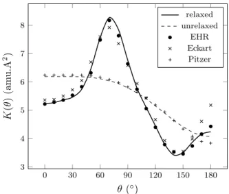
obtained by Fourier series development of the optimized internal coordinates, and are presented in Supplemen-tary Information 1. The kinetic function calculated us-ing our numerical approach is presented on figure 3 (solid line), and compared to those reported by Vansteenkiste et al.11 and Wong et al.9. A very good agreement is
observed between the 3 studies, the difference from the Eckart method at θ≈ 180◦ being most likely attributed
to the different level of theory used in the study of Wong et al. for geometry optimization (MP2). We also present in figure 3 the kinetic function computed when the relax-ation of the geometry with respect to θ is not taken into account (fi(θ) = 0 ∀i, dashed line). As it can be seen,
the kinetic function is strongly affected and gives values in close agreement with those presented by Wong et al.9
C1 C2 1 1.34 H3 1 1.09 2 121.8 H4 1 1.09 3 116.6 2 180 + f1(θ) C5 2 1.46 + f2(θ) 1 124.3 + f3(θ) 3 180 + f4(θ) H6 2 1.09 1 119.4 3 f5(θ) C7 5 1.34 2 124.3 + f3(θ) 1 −180 + θ H8 5 1.09 2 116.2 1 θ + f7(θ) H9 7 1.09 5 121.5 2 f8(θ) H10 7 1.09 5 121.8 2 180 + f9(θ)
TABLE I. Functional Z-Matrix definition of the torsional motion of the 1,3-Butadiene. The definition of the relax-ation functions fi(θ) are given as supplementary informations.
Lengths are in Angstrom and angles in degrees.
0 30 60 90 120 150 180 3 4 5 6 7 8 θ (◦) K (θ ) (am u .A 2 ) relaxed unrelaxed EHR Eckart Pitzer
FIG. 3. Comparison between the kinetic function calculated in this work (lines) and the kinetic function obtained using the Extended Hindered Rotor model11 (EHR), the Eckart
method9and the Pitzer method57(presented by Wong et al.9). Solid line: flexible torsion (fi(θ)�= 0); dashed line: rigid
ro-tation (fi(θ) = 0).
calculated using the Pitzer method57. Because the Pitzer
values are also based on relaxed geometries, this demon-strates that the Pitzer method actually fails to take into account the dynamic influence of the relaxation on the kinetic energy.
3. Calibration of the potential energy surface
The model used to describe the PES of the torsional motion accounts for two physical contributions: (i) the contribution of the intrinsic torsional energy of the C5-C2
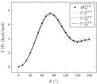
0 30 60 90 120 150 180 0 2 4 6 8 θ (◦) V (θ ) (k cal /m ol ) DDF T 19 [V ]DF T 5 [V ]DF T 10 [V ]DF T 20
FIG. 4. 95% confidence interval of the posterior PES using the data set DDF T
n with n = 5 (dotted line), n = 10 (dashed
line) and n = 20 (solid line). Filled circles represent the data set DDF T
19 .
sp2chemical bond, and (ii) the contribution of a repulsive
part, representing the steric repulsion between the atoms H9and H4during the torsion. Using the definition of the
repulsive part of a Lennard-Jones type potential, and a modified cosine function to account for the sp2 torsion
energy, the PES is defined using the 3 parameters a0, a1,
and a2 by: V (θ) =a1 2 (1− cos (2θga0(θ))) + a2 � dVDW | �R9(θ)− �R4(θ)| 9 − dVDW | �R9(0)− �R4(0)| 9� (26) where dVDW is taken equal to 2.4 ˚A(sum of the van
der Waals radii of the hydrogen atoms), and ga0(θ) =
1− a0(1− cos(2θ)). The function ga0 adds degrees of
freedom to model the bonding contribution of the sp2
tor-sional energy, and one can verify that ga0(θ) = ga0(−θ)
as well as ga0(−180) = ga0(180) = ga0(0) = 0. The
term −dVDW/| �R9(0)− �R4(0)|9 in the equation ensures
the condition V (0) = 0. The stochastic PES model M contains four parameters to calibrate: the three involved in Eq.(26) (a0, a1, a2), and the variance (σ2M).
In order to study how the ab initio data inform the PES parameters, different datasets are used for the inference process. They are noted DXn where X ∈
{DF T, CC} stands for the level used for the electronic energy calculations, and n is the number of values in-cluded (in uniform repartition in [0; 180 ◦]). The prior PDFs, the 95 % confidence intervals (CIs) based on the posterior PDFs, and the posterior means are presented in table II.
We first comment on the results obtained using the DFT datasets. It is shown in rows 3 to 8 that the 95% CI is considerably narrowed around the mean value for each parameter each time the dataset size increases. Also, the posterior mean value < ai > is already accurately
predicted when only 5 points are used. However, the parameter uncertainties remain large at this level. The mean of the variance shows a different behavior: its value keeps decreasing when the amount of data increases. It reaches 1.25×10⁻³kcal2/mol2(e.g. < σ
M>= 3.5×10⁻²
kcal/mol) when 20 points are used. The 95% CIs [V ]DF T n
(n = 5, 10, 20) are presented in figure 4 and compared to the DDF T19 data set. The figure confirms the quality
of the proposed model and is able to reproduce almost perfectly the ab initio results when a sufficient amount of data points is used. It is worth mentioning that the uncertainty on the posterior PES (maximum here at≈ 90
◦ and ≈ 180 ◦) highlights the most relevant volume of
the configurational space in which data are needed to improve the calibration process.
We now look at the posterior PDFs of model param-eters obtained using the data set DCCn (n = 2, 3, 5)
pre-sented on the four last rows of table II. In this case, we calibrate model parameters except for σ2
M, which is set
to be 1.25× 10⁻³ kcal2/mol2. In other words, we assume
that the model error obtained by the DF T level of the-ory is close to the realistic estimation of the true model error. As can be seen on table II, this assumption is rea-sonable since [V ]CC
5 is already very narrow (and actually
converged) for all the parameters even when 5 points are used. It is also shown that using 2 points (at 0 ◦ and 180◦) is not enough to infer a
0 and a2 (posterior PDFs
approximately equal to the prior PDFs), while a third point at 90 ◦ allows a considerable reduction of the
un-certainty on a2. These results are illustrated on figure 5,
which presents the uncertainty domain of the posterior PES for these three datasets. Comparing [V ]CC
5 a
poste-riori with the DCC19 dataset demonstrates that the DFT
level of theory is fully able to estimate the absolute model error for this case as the data points are almost perfectly encapsulated in [V ]CC
5 (assuming that the
CCSDT/aug-cc-dvpz level of theory gives the exact PES).
4. Forward Problem: Partition function
The 95% CI of the posterior partition function [QLAM]DF T using the DDF Tn=5, 10, 20datasets are presented
in figure 6. The results are normalized to the par-tition function obtained using an HO approximation. The mean value of the posterior partition function us-ing DDF T5 is also presented. As for the PES results, the
95% CI becomes very narrow as soon as 10 points are used, and the mean value < Q >DF T
5 is already almost
converged. The fact that the [Q]X
n are centered around
1 at low temperature (T < 400 K) is important because it demonstrates that the method presented here to treat the 1D LAM has a sufficient capability to perfectly
re-0 30 60 90 120 150 180 0 2 4 6 8 10 θ (◦) V (θ ) (k cal /m ol ) [V ]CC 2 [V ]CC 3 [V ]CC 5 0 30 60 90 120 150 180 0 2 4 6 8 10 θ (◦) V (θ ) (k cal /m ol ) DCC 2 DCC3 DCC 5 DCC 19
FIG. 5. 95% CI of the posterior PES using the data set DCC n
with n = 2 (dotted line), n = 3 (dashed line) and n = 5 (solid line). The circles, crosses and empty circles represent the cor-responding data set respectively. The filled circles represent the data set DCC
19 . a0× 102 a1 a2 σ2M× 103 Prior [1;10] [1;10] [1;10] [0;2000] [.]DF T5 [2.22;9.15] [2.32;3.87] [6.65;8.34] [25.8;1332.2] [.]DF T 10 [4.82;6.84] [2.92;3.35] [7.28;7.72] [0.34;154.8] [.]DF T 20 [5.54;5.99] [3.05;3.14] [7.46;7.53] [0.18;3.9] < . >DF T 5 5.95 3.15 7.45 196.02 < . >DF T 10 5.92 3.17 7.5 16.30 < . >DF T 20 5.79 3.10 7.49 1.25 σ2 M= cst [.]CC 2 [1.36;9.52] [2.73;2.84] [1.53;9.59] 1.25 [.]CC 3 [1.42;9.6] [2.74;2.84] [5.72;6.28] 1.25 [.]CC 5 [6.89;7.78] [2.75;2.85] [6.02;6.14] 1.25 < . >CC 5 7.33 2.80 6.08 1.25
TABLE II. Definition of the parameter’s priors, and descrip-tion of the parameter’s posterior for each dataset used in the paper. Units: a0: no unit, a1: kcal/mol, a2: kcal/mol, σM:
kcal/mol.
produce the harmonic approximation results in the low temperature limit.
The total partition function of 1,3-butadiene is ob-tained by multiplication of the LAM partition function by the FR and FO partition functions. To compute the FHO partition function, we consider the system constituted by two stable complexes, characterized by the normal mode frequencies at θ = 0 ◦ and θ = 145 ◦ (the normal mode
frequencies are presented as supplementary information).
0 500 1,000 1,500 1 1.2 1.4 1.6 1.8 T (K) QLA M (T ) /Q HO (T ) [QLAM]DF T5 [QLAM]DF T10 [QLAM]DF T20 < QLAM>DF T5
FIG. 6. 95% CI of the posterior torsional partition function using the data set DDF Tn with n = 5 (dotted line), n = 10
(dashed line) and n = 20 (solid line). Filled circles: mean of the posterior torsional partition function using DDF T
5 .
Re-sults are normalized by the HO partition function.
0 500 1,000 1,500 1 1.5 2 T (K) Q tot (T ) /Q tot RRH O (T ) [Q]CC 5 [Q]DF T 20 EHR Pert
FIG. 7. Comparison between the 95% confidence interval of the posterior partition function of the butadiene using DDF T20
(dashed line) and DCC
5 (solid line, σM2 = 1.25 10−3). Crosses:
Pert method58, circles: EHR method11. Results normalized
to the RRHO partition function.
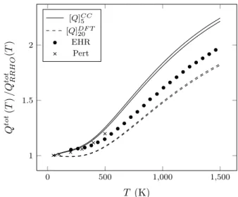
It should be noted that the PES uncertainty also affects the FR and FO partition functions through Eq. (6) and Eq. (25). The 95% CI of the posterior partition function of 1,3-butadiene using the DCC5 (with σ2
Mkeeped fixed at
1.25 10−3 kcal2/mol2) and DDF T
20 datasets are presented
on figure 7 and compared to the results presented by Wong and Raman58(Pert model) and those presented by
Vansteenkiste et al.11(EHR model). The results are
nor-malized by the partition function obtained using a Rigid Rotor Harmonic Oscillator approximation (RRHO). We first compare our prediction using DCC5 with the low
tem-perature results presented by Wong and Raman58using
their Pert method. The comparison is meaningful be-cause the same level of theory has been used to compute the PES, and also because the Pert method used rep-resents most likely the best model available in the lit-erature. However, this fully coupled quantum method is computationally expensive, which explains why no re-sults for temperatures higher than 500 K have been pre-sented. Although our predictions slightly overestimate the partition function, the behavior of the curves is very similar, and the results stay very close to each other. The small overestimation comes from either the simplification introduced by our treatment and/or from differences in the RRHO reference partition function. We now com-pare the results obtained by Vansteenkiste et al.11(EHR
method) and our results using the DDF T20 data set. The
same DFT method used to compute the PES is shared by the two studies; however, Vansteenkiste et al. consider a larger basis set in their work (6-311G(d,p)). The two PESs are nevertheless similar, as reflected by the small difference of the torsional barrier height (0.1kcal/mol). As can be seen in the figure, the behavior of the parti-tion funcparti-tion curves are very similar, essentially differing by a small translation factor. This factor seems to be an artifact involved in the EHR method as the partition function does not converge to 1 at the limit of low tem-peratures.
The model 1D LAM method proposed in this paper is able to account for 1D torsional motion with an ac-curacy comparable to the best methods presented until now. It is worth recalling that only 2 normal mode anal-yses have been realized here, while they have been con-ducted all over the configurational space in the studies of Vansteenkiste et al.11 and Wong and Raman58. Also,
this efficient formalism, in terms of computational time, further allows it to be used in conjunction with an un-certainty quantification algorithm.
B. Kinetic rate of CH3+ H→ CH4 in the high pressure
limit
The reaction rate of the CH3+H recombination is
com-puted at the high pressure limit using Variational Tran-sition State Theory (VTST) with Variational Reaction Coordinate (VRC) and spherical Dividing Surfaces (DS) in the canonical ensemble. In the present case, the DS is parameterized using one pivot point �p attached to the CH3 part, around which the approaching H∗ atom is
al-lowed to rotate. The optimal DS (noted DS∗), defin-ing the transition state, is optimized for every tempera-ture in a way that it is associated to a minimal partition
function59,60: QDS∗(T ) = min � p,s[Q � p,s DS(T )] (27)
where s is the reaction coordinate (separation �p−H∗),
and Q�p,sDS(T ) is the partition function of the DS defined by s and �p. The high pressure reaction rate is calculated using the standard TST assumptions and is given by52:
k(T ) = kBT h
Q�p,xDS∗
QCH3(T )QH(T )
exp (V∗/kBT ) (28)
where h is Plancks constant, QCH3 and QHthe partition
functions of the methyl and hydrogen radicals respec-tively, and V∗ is the electronic barrier height associated
with the CH3+H DS∗. Over the small amplitude motion
involved in the system, the CH3umbrella motion changes
quite substantially and may need to be included in a FO partition function. However, Klippenstein et al.16 have
shown that its influence is negligible with at most a 2 % increase of the reaction rate for temperatures below 2400 K. In this work, the small amplitude motions are then supposed uncoupled to the reactional motion, and the reaction rate expression is simplified into:
k(T ) = kBT h Q2D DS∗(T )QFRDS∗ Qtrans&rot CH3 (T )QH(T ) exp (V∗/kBT ) (29) where Q2D
DS∗ is the partition function of the H∗ motion
on the DS∗, QFR
DS∗ the effective overall rotation partition
function of the DS, and Qtrans&rot
CH3 the partition function
of the overall translational and rotational motion of CH3.
1. Electronic structure calculation
Ground state electronic energies are calculated us-ing the CR-CC(2,3)61,62/aug-cc-pvdz55,56 level of theory.
The CR-CC(2,3) method is an improvement over the CCSD(T) approach to overcome its deficiencies in de-scribing systems involving biradical character63.
Geom-etry optimizations are carried out at the UB3LYP53
/6-31G(d)54 level of theory. All the electronic calculations
have been performed using the GAMESS code2.
2. Kinetic function
The kinetic energy of the DS is obtained by defining the functional Z-Matrix associated with the H∗ 2D mo-tion. Because of the C3 symmetry of CH3, the DS is
parameterized by 2 parameters. The first parameter is the distance x between the pivot point �p, lying in the C3
axis of symmetry of CH3, and the carbon atom, taken
as the origin. We denote from now on �p = x. The sec-ond parameter is the distance s between the approaching H∗ atom and the pivot point. The functional Z-Matrix
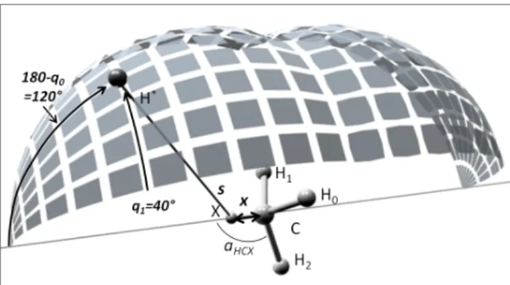
FIG. 8. Illustration of a typical bi-faceted dividing surface of the CH3+H→ CH4 reaction.
symmetry is imposed to the system, and the relaxation of the CH3 part is taken into account to some extent by
using the functions a(|CH→∗|) (interpolation between the optimized values on the MEP).
It has been shown that a limitation of the spherical dividing surfaces is that they can account for artificial contributions to the reaction rate when multiple reac-tion paths are present12,13. To avoid this overestimation,
a multifaceted dividing surface are used, composed by the envelope of spherical DSs centered around a reactive channel specific pivot point. Considering the equivalence of the two association channels for the H∗ addition on
CH3, a typical dividing surface for the reaction is
illus-trated on figure 8. To compute the DS partition function, the integration domain defined in Eq. (5) has to be re-stricted to:
q0∈ [qmin0 , π]
q1∈ [0, π/3]
(30) where qmin
0 = arcsin(x/s) is the solid angle from X
defin-ing the intersection of the two spherical DS. The overall symmetry number of the irreducible integration domain is then 12. Since this number takes into account the two reaction paths, no symmetry number has to be consid-ered in the overall rotational partition function of both CH3 and the DS. C X 1 x H0 1 1.09 2 a(| → CH∗|) H1 1 1.09 2 a(| → CH∗|) 3 120 H2 1 1.09 2 a(| → CH∗|) 4 120 H∗ 2 s 1 q0 3 q1
TABLE III. Z-Matrix definition of the Dividing Surface pa-rameterized by the reaction coordinate s and the pivot point x. Lengths in Angstrom, angles in degrees.
3. Calibration of the PES
The PES of the CH3/H∗interaction accounts for three
contributions: (i) the stretching energy of the C-H∗bond
(noted Vstr), (ii) the bending energy of the HiCH∗degree
of freedom (noted Vbend), and (iii) the steric repulsion
energy between the Hi and H∗. The stretching energy
Vstr is written as a Morse-like function of | →
CH∗ | with an origin of energy taken at the products state:
Va0,a1 str = De � 1− exp(−a0(| → CH∗| − req)a1) �2 − De (31) where De = 107.7 kcal/mol is the dissociation energy,
req = 1.09 ˚A is the equilibrium bond length, a0 and a1
are the first two parameters of the PES model. Note that the function is defined only for|CH→∗ | > req. The
bending energy is modeled by a simple cosine function, with a barrier height equal to the dissociation energy at the angle αXCH∗ =±π/2:
Vbend=
De− Vstr(q0, q1)
2 (1− cos(αXCH∗)) (32) Finally the PES also accounts for the spherical repulsion between the passive hydrogen atoms Hi and H∗:
Va2,a3 rep = a2 � i=0,1,2 σHH |H→iH∗| a3 − σHH |H→iH∗0| a3 (33) where σHH = 2.4 ˚A with a2 and a3 being the last two
parameters, and H∗0 is the corresponding position of H∗
on the MEP (at the same C− H∗ separation). The term �
σHH
|H→iH∗0|
�a3
allows a cancellation of the steric interaction energy on the MEP. The PES is the sum of these three contributions, and are defined through the four parame-ters ai, i = 0, ..., 3:
Vai(q) = Va0,a1
str (q) + Vbend(q) + Vrepa2,a3(q) (34)
The geometries used to compute the electronic energies are defined by the Z-Matrix presented in table III with x = � = 10−5 (in order to preserve a non-ambiguous
definition of the C3 axis). The 50 data points collected
are divided in two groups: one is used to infer the PES model (noted D∗), and the second is used to validate it for extrapolation (noted D). The dataset D∗ contains 25 points in the relevant space of the PES for reaction rate calculation and is constituted by:
(a) 10 points on the MEP (q0 = q1 = 0) from s = 2.0
to s = 3.8 ˚A
(b) 15 points out of the MEP defined by the combination s ∈ {2.0, 2.4, 2.8˚A} ⊗ q0 ∈
{20, 40, 60, 80, 100◦} ⊗ q 1= 0
1.7 1.8 1.9 2 0 5 10 a0(˚A−a1) p( a0 |D ∗,M ) (a) 1 1.5 0 2 4 a1(no unit) p( a1 |D ∗,M ) (b) 2 4 6 8 10 0 0.2 0.4 a2 (kcal/mol) p( a2 |D ∗,M ) (c) 2 3 0 0.5 1 1.5 a3(no unit) p( a3 |D ∗,M ) (d)
FIG. 9. Posterior PDF, p(ai|D∗, M ), (a), (b), (c), (d) for
respectively i=0, 1, 2, 3.
The D data set collects the energies of the corresponding geometries of (b) at q1 = 30◦ as well as 10 other points
at s = 1.6 ˚A. The prior intervals, the posteriors means, and 95 % confidence intervals are presented in table IV, and the 4 posteriors p(a|D∗, M ) are presented in figure 9. We confirm here that the Morse potential (defined for a1 = 1) is not the most appropriate to describe the
MEP, and a value of a1= 1.25 is the most probable value.
The mean value of a3 is surprisingly low for a repulsion
term: in a Van Der Waals force field, the exponent of the repulsive part is usually taken between 9 and 12.
a0 a1 a2 a3 σM2
Prior [0;10] [0;10] [0;10] [0;10] [0;10] [.] [1.75;1.87] [1.22;1.43] [2.13;6.04] [2.12;2.87] [1.6;2.8] < . > 1.82 1.27 4.12 2.53 2.59
TABLE IV. The prior PDFs of the parameters, and 95% CIs ([.]) based on the posterior PDFs, and the posterior mean values (< . >). Units: a0: ˚A−a1, a1: no unit, a2: kcal/mol,
a3: kcal/mol, σM: kcal/mol.
We compare on figure 11 the 95 % CI of the pos-terior MEP ([V ]) with the data points of D∗ (black symbols) and D (white symbols) included in the MEP. We also report on this figure the ab initio results at the CASPT2/aug-cc-pVQZ17, full-CI/6-31G(d)64 and
CCSD(T)/6-31G(d)17 level of theories presented in the
2 2.5 3 3.5 4 −80 −60 −40 −20 0 2 kcal/mol s (˚A) V (s ;0; 0) (k cal /m ol ) [V ] CASPT2 full CI CCSD(T) D D∗
2
2.5
3
3.5
4
−80
−60
−40
−20
0
2 kcal/mol
s (˚
A)
V
(s
;0;
0)
(k
cal
/m
ol
)
[V ]
CASPT2
full CI
CCSD(T)
D
D
∗
FIG. 10. Comparison between the predicted 95% confi-dence interval of the MEP ([V ]), the datasets D and D∗ and the ab initio results presented in literature. Lines: [V ]; black circles: D∗, empty circles: D. Grey symbols: lit-terature results; asterisks: CCSD(T)/6-31G(d)17, crosses: CASPT2/aug-ccVQZ17, times: full CI/6-31G(d)64. Origin
of energy: V (4 ˚A, 0, 0).
literature. The uncertainty of the PES model is under 2 kcal/mol for separations higher than 2.0 ˚A, and coin-cidently encapsulates the results obtained at the full CI and CASPT2 level of theory. As already reported17, the
CCSD(T) level of theory is not able to properly estimate the energy of the system for intermediate separation. The comparison between the PES model and the direct ab ini-tio data is pursued in figure 11 for out-of-MEP situaini-tions. The black and white symbols still represent the D∗ and D data sets respectively. The approximation of the PES model is very satisfying. Even for extrapolated values at low separation (s = 1.6 ˚A) the model still performs well with the hindering domain being correctly predicted within 10%.
4. Forward propagation to the high-pressure recombination rate
The 95 % CI ([k]) and the mean (< k >) of the poste-rior high pressure reaction are presented in figure 12 with the available experimental measurements65–67 and the
VTST-VRC theoretical predictions presented by Klip-penstein et al.16and Harding et al.17. The experimental
measures have been converted from the k0 values of the
original experimental works in the same way presented by Klippenstein et al.16. The confidence intervals
pre-dicted by our approach are in very good agreement with the experimental values as well as with the theoretical calculations. Our calculations are mainly limited by two methodological factors. First, the representation of the
−90 −60 −30 0 30 60 90 −80 −60 −40 −20 0 20 40 q0(◦) V (si ˚ A; q0 ;0) (k cal /m ol ) Ds=2.8 Ds=2.4 Ds=2. Ds=1.6 −90 −60 −30 0 30 60 90 −80 −60 −40 −20 0 20 40
Data not used [V ] & data used
s=1.6 s=2. s=2.4 s=2.8 s=2.8 q0(◦) V (si ˚ A; q0 ;0) (k cal /m ol ) [V ] D∗ s=2.8 D∗s=2.4 D∗s=2.0
FIG. 11. Comparison between the predicted 95% confidence interval of the PES ([V ]) with the datasets D and D∗. Lines:
[V ]; black circles: D∗, empty circles: D. Origin of energy: V (4 ˚A, 0, 0).
dividing surface does not constitute a perfect DS and it is associated with an overestimation of the reaction rate. The works of Klippenstein et.al.16have shown that by
us-ing both VTST-VRC and a direct dynamic method, the spherical DS for the CH3+H→ CH4reaction is associated
with a 9 % overestimation, approximately independent of the temperature. The doubly faceted DS used here leads to an even lower recrossing factor. The second limitation is the restriction of the statistical study to the canoni-cal ensemble. In other works12, the associated error is
evaluated at approximately 20 %. The overestimation of the reaction rate coming from the canonical analysis is probably compensated to some extent by the PES model which predicts a slightly higher hindrance effect at high separation (the ab initio data are close to the bottom boundary of the confidence interval at the s = 2.8 ˚A case on figure 11).
To finish this study, we comment on the difference in the PES representation used here and in the works pre-sented by Harding et al.17 and Klippenstein et al.16. In the works of Klippenstein et al.16, a combined Fourier
se-ries/3D spline fitting procedure is used to obtain a four dimensional PES representation (the umbrella motion is also explicitly considered). If the fit is almost exact, it has been achieved using 798 ab initio calculations in the three dimensional space analyzed here. Klippenstein et al. have also used the analytical PES presented by Hirst-Hase to compute the reaction rate. This model, in ad-dition to having required the manual optimization of al-most 20 parameters, does not provide any indication of the associated model error. In the study of Harding et al.17, an on-the-fly method is used to compute the PES.
The number of quantum calculations has not been pre-sented, but, assuming that ten points are used to
inte-0 500 1,000 1,500 1 2 3 4 5 T (K) k× 10 10 (c m 3/m ol ec u le /s ) Brouard et.al. Seakins et.al. Su et.al. 0 500 1,000 1,500 1 2 3 4 5 T (K) k× 10 10 (c m 3/m ol ec u le /s ) [k] < k > Harding et.al. Klippenstein et.al. Hirst-Hase PES
FIG. 12. Comparison of the high pressure CH3+H
recombi-nation rate predicted by this work (black lines: [k], squares: < k >) with other theoretical calculations (gray lines) and the experimental values (crosses66, asterisks67, times65). Gray lines: calculations using different representation of the PES; full line: on the fly calculation17, dashed line: 4D
mathemat-ical fit16, dotted line Hirst-Hase PES.
grate the partition function along q0and q1and 10 points
to optimize ds and dx, this already results in 10,000 ab initio calculations. We recall that our model, even if associated with a 1.5 uncertainty factor on the reaction rate, is based on 4 parameters and has been set using 25 ab initio calculations for the calibration step (and 25 to examine the extrapolation capabilities). The restriction to the canonical ensemble is another issue which does not need more PES calculations to be overcome.
IV. CONCLUSIONS
We have presented in this work an original approach for the computation of statistical properties of molecular systems involving a large amplitude motion. The objec-tives were to propose: (i) a simple and general procedure to compute the kinetic energy of a LAM, (ii) a general procedure to calibrate an analytical PES using ab initio data, and (iii) a rigorous quantification of the uncertainty of the PES model, and their propagation to the QoI(s). Two typical and different test cases have been consid-ered for assessing the methodology: (i) the study of 1-3 butadiene, involving non trivial features like coupling of modes or a highly variable kinetic function, and (ii) the study of the CH3+H recombination, for which a
VTST-VRC approach is needed to compute an accurate reaction rate.
We proposed to compute the kinetic energy of a LAM based on a functional Z-Matrix formalism, e.g. a Z-Matrix, in which the internal DOF are defined with
re-spect to some generalized coordinates. The results ob-tained are exact within numerical precision and are in total agreement with previous exact methods. The par-ticular advantage that our approach offers is its practi-cal convenience. Indeed, for a typipracti-cal LAM, the internal Z-Matrix coordinates naturally describes the configura-tional space of the motion and are much more suited than Cartesian coordinates. Also, the possibility to in-clude ghost atoms in the Z-Matrix to represent a virtual pivot point is an additional important advantage when one wishes to study dissociation reactions involving loose complexes. Finally, the method applies equally regard-less of the number of generalized coordinates or their type (length, angle, reaction path-like coordinate).
Furthermore, the calibration of parameters for the ana-lytical PES from ab initio calculations has been achieved using Bayesian theory. The two examples treated have allowed us to point out different and interesting features of this approach. The most important one, which is crit-ical to the derivation of analytcrit-ical models, is that the PES model uncertainty is properly evaluated, and can be propagated to the QoI. We have also shown that, pro-viding an adequate PES model is used, narrowing the QoI confidence interval needs significantly fewer data points than other methods, which does not exploit any particu-lar physical contribution of the interaction energy. This is particularly true when the dimension of the problem increases. For instance, in the study of the CH3+H
re-combination rate, we were able to use only 25 data points to calibrate the 3D PES in order to compute a reaction rate within an uncertainty factor of 1.5 (coming from the PES model). This corresponds to a typical reduction of one or two orders of magnitude in the amount of data points needed with respect to previous study. However, it is clear that this approach is relevant when the condi-tion that a satisfactory model of the interaccondi-tion energy is provided. Even for complex force fields, we have shown here that for the two studied applications, accurate mod-els can be based on simple contributions: Morse-like type potentials for bond stretching, cosine-like functions for bending and torsional motion, and steric repulsion for non bonded atoms. We believe that these types of poten-tials should hold for the majority of torsional and bond breaking context studies. Finally, for the 1,3 butadiene application, we have discussed the possibility of perform-ing a dual level inference process. While it is not possible to generalize the results, it was shown that the B3LYP/6-31G(d) level of theory was almost perfectly able to com-pute the true (or absolute) model error, even if the PES is not accurately rendered at this level. As knowing the model error is a useful information, which considerably reduces the required amount of data needed to obtain a given accuracy on the QoI, this property would be of a particular interest for the calibration of high level PESs at a minimum computational cost.
Appendix A: Supplementary Information
1. SI 1. Fourier series development of the functions fi(θ)
for Butadiene (see table I)
f1 = −8.15 cos(q)10−2 + 2.05 sin(q)10−1 + 3.55 sin(2q)10−1 + 7.38 sin(3q)10−1 − 3.42 sin(4q)10−1
f2 = −3.42 cos(q)10−3 + 1.05 sin(q)10−5 − 1.08 cos(2q)10−2 − 4.21 cos(3q)10−3 f3 = −1.06 cos(q) − 8.48 sin(q)10−4 + 4.93 cos(2q)10−1 − 3.10 cos(3q)10−1
+ 3.43 cos(4q)10−1
f4 = −5.95 cos(q)10−2 − 1.05sin(q) − 2.28 sin(2q) − 2.49 sin(3q) + 3.92 sin(4q)10−1+ 3.93 sin(5q)10−1+ 2.12 sin(6q)10−1 f5 = −7.91 cos(q)10−2 − sin(q) + 9.31 cos(2q)10−3 + 3.57 sin(2q)
− 8.77 cos(3q)10−3+ 7.90 sin(3q)10−1+ 5.39 cos(4q)10−2 − 5.46 sin(4q)10−1 + 2.47 cos(5q)10−2 − 3.27 sin(5q)10−1 − 9.89 cos(6q)10−3 + 6.02 sin(6q)10−3 − 1.41 cos(7q)10−2+ 1.1 sin(7q)10−1+ 5.32 cos(8q)10−3+ 8.94 sin(8q)10−2 + 6.05 cos(9q)10−2
f6 = −1.056 cos(q) − 2.61 sin(q)10−3 + 4.87 cos(2q)10−1 − 3.08 cos(3q)10−1 + 3.47 cos(4q)10−1
f7 = 8.36 cos(q)10−2 − 5.69 sin(q)10−2 − 7.99 cos(2q)10−2 − 5.7 sin(2q) + 4.04 cos(3q)10−2 − 3.28 sin(3q) − 1.14 cos(4q)10−3 + 1.03 sin(4q) − 1.33 cos(5q)10−2+ 6.22 sin(5q)10−1
f8 = 5.9 cos(q)10−3 − 1.2170 sin(q) − 1.78 cos(2q)10−2 − 2.68 sin(2q) + 1.2 cos(3q)10−3 − 3.27 sin(3q) + 1.03 cos(4q)10−2 + 7.85 sin(4q)10−1 + 5.8 cos(5q)10−3+ 4.46 sin(5q)10−1+ 2.42 sin(6q)10−1 − 4.9 cos(7q)10−3 − 1.9 sin(7q)10−1+ 6.83 cos(8q)10−4 − 1.52 sin(8q)10−1 − 1.10 cos(9q)10−2 f9 = 2.5 cos(q)10−3 − 1.11 sin(q) − 2.26 sin(2q) − 2.49 sin(3q) + 3.66 sin(4q)10−1
+ 3.81 sin(5q)10−1+ 1.81 sin(6q)10−1
(A1)
2. SI 2. Normal mode frequencies of the 1,3 Butadiene at θ = 0 and θ = 145◦
List of the normal mode frequencies of the 1,3 Butadi-ene for θ = 0◦: f (cm−1) ={176.97 (torsion), 297.8, 515.78, 539.96, 781.87, 907.07, 927.71, 931.51, 1002.42, 1010.99, 1063.85, 1240.02, 1328.87, 1331.52, 1434.8, 1496.2, 1676.49, 1729.1, 3127.6, 3143.88, 3168.83, 3176.04, 3233.98, 3255.78} (A2)
List of the normal mode frequencies of the 1,3 Butadiene for θ = 145◦: f (cm−1) ={186.12 (torsion), 273.93, 476.51, 625.72, 761.55, 890.42, 934.59, 936.96, 1024.91, 1041.86, 1078.38, 1112.56, 1323.89, 1356.82, 1455.35, 1483.65, 1689.57, 1715.05, 3109.54, 3142.19, 3150.97, 3160.79, 3232.96, 3239.67} (A3)
1M. J. Frisch, G. W. Trucks, H. B. Schlegel, G. E. Scuseria, M. A.
Robb, J. R. Cheeseman, J. J. A. Montgomery, T. Vreven, K. N. Kudin, J. C. Burant, J. M. Millam, S. S. Iyengar, J. Tomasi, V. Barone, B. Mennucci, M. Cossi, G. Scalmani, N. Rega, G. A. Petersson, H. Nakatsuji, M. Hada, M. Ehara, K. Toy-ota, R. Fukuda, J. Hasegawa, M. Ishida, T. Nakajima, Y. Honda, O. Kitao, H. Nakai, M. Klene, X. Li, J. E. Knox, H. P. Hratchian, J. B. Cross, V. Bakken, C. Adamo, J. Jaramillo, R. Gom-perts, R. E. Stratmann, O. Yazyev, A. J. Austin, R. Cammi,
C. Pomelli, J. W. Ochterski, P. Y. Ayala, K. Morokuma, G. A. Voth, P. Salvador, J. J. Dannenberg, V. G. Zakrzewski, S. Dap-prich, A. D. Daniels, M. C. Strain, O. Farkas, D. K. Malick, A. D. Rabuck, K. Raghavachari, J. B. Foresman, J. V. Ortiz, Q. Cui, A. G. Baboul, S. Clifford, J. Cioslowski, B. B. Stefanov, G. Liu, A. Liashenko, P. Piskorz, I. Komaromi, R. L. Martin, D. J. Fox, T. Keith, M. A. Al-Laham, C. Y. Peng, A. Nanayakkara, M. Challacombe, P. M. W. Gill, B. Johnson, W. Chen, M. W. Wong, C. Gonzalez, and J. A. Pople, “Gaussian 03, Revision C.02.” Gaussian, Inc., Wallingford, CT, 2004.
2M. W. Schmidt, K. K.Baldridge, J. A. Boatz, S. T. Elbert,
M. S. Gordon, J. J. Jensen, S. Koseki, N. Matsunaga, K. A. Nguyen, S. Su, T. L. Windus, M. Dupuis, and J. A. Montgomery J.Comput.Chem., vol. 14, p. 1347, 1993.
3S. W. Benson, The foundations of chemical kinetic. Kriegler,
Malabar, 1982.
4K. S. Pitzer and W. D. Gwinn J. Chem. Phys, vol. 10, p. 428,
1942.
5J. E. Kilpatrick and K. S. Pitzer J. Chem. Phys., vol. 17, p. 1064,
1949.
6G. Katzer and A. F. Sax J. Phys. Chem. A, vol. 106, p. 7204,
2002.
7J. Pfaendtner, X. Yu, and L. BroadBelt Theor. Chem. Acc.,
vol. 118, p. 881, 2007.
8A. L. L. East and L. Radom J. Chem. Phys., vol. 106, p. 6655,
1997.
9B. M. Wong, R. L. Thom, and R. W. Field J. Phys. Chem. A,
vol. 110, pp. 7406–7413, 2006.
10J. Gang, M. J. Pilling, and S. H. Robertson Chemical Physics,
vol. 231, pp. 183–192, 1998.
11P. Vansteenkiste, V. V. S. D. Van Neck, and M. Waroquier J.
Chem. Phys., vol. 124, p. Art. No. 044314, 2006.
12Y. Georgievskii and S. J. Klippenstein J. Chem. Phys., vol. 118,
no. 12, pp. 5542–5455, 2003.
13S. Robertson, A. F. Wagner, and D. M. Wardlaw J. Phys. Chem.
A, vol. 106, pp. 2598–2613, 2002.
14S. C. Smith J. Phys. Chem., vol. 111, no. 1999, p. 1830. 15S. Robertson, A. F. Wagner, and D. M. Wardlaw J. Chem. Phys.,
vol. 113, p. 2648, 2000.
16S. J. Klippenstein, Y. Georgievskii, and L. B. Harding
Proceed-ings of the Combustion Institute, vol. 29, pp. 1229–1236, 2002.
17L. B. Harding, S. J. Klippenstein, and A. W. Jasper Phys. Chem.
Chem. Phys., vol. 9, pp. 4055–4070, 2007.
18H. B. Schlegel J.Comput.Chem., vol. 24, pp. 1514–1527, 2002. 19G. C. Schatz, Reaction and Molecular Dynamics, vol. 75 of
Lec-ture Notes in Chemistry. Springer, Berlin, 2000.
20G. C. Schatz Rev. Mod. Phys., vol. 61, p. 669, 1989.
21G. Ochoa de Aspuru and M. L. Hernandez, Reaction and
Molec-ular Dynamics. Lecture Notes in Chemistry, Springer, Berlin, 2000.
22D. K. Hoffman, G. W. Wei, D. S. Zhang, and K. D. J. Phys. Rev.
E., vol. 57, p. 6152, 1998.
23T. Ishida and G. C. Schatz J. Chem. Phys., vol. 107, p. 3558,
1997.
24G. C. Maisuradze, D. L. Thompson, A. F. Wagner, and
M. Minkoff J. Chem. Phys., vol. 119, p. 10002, 2003.
25G. K. Chawla, G. C. McBane, P. L. Houston, and G. C. Schatz
J. Chem. Phys., vol. 88, p. 5481, 1988.
26G. C. Schatz, A. Papaioannou, L. A. Pederson, L. B. Harding,
T. Hollebeek, T. S. Ho, and H. Rabitz J. Chem. Phys. 107, vol. 107, p. 2340, 1997.
27A. J. C. Varandas Adv. Chem. Phys., vol. 74, p. 255, 1988. 28J. T. Murrel, S. Carter, S. C. Farantos, P. Huxley, and A. J. C.
Varandas, Molecular Potential Energy Functions. Wiley, 1988.
29A. Lagana, G. O. Aspuru, and E. Garcia J. Chem. Phys.,
vol. 108, p. 3886, 1998.
30A. K. Rappe, C. J. Casewit, K. S. Colwell, W. A. Goddard III,
and W. M. Skiff J. Am. Chem. Soc., vol. 114, p. 10035, 1992.
31J. W. Ponder and D. A. Case Adv. Prot. Chem., vol. 66, pp. 27–
85, 2003.
32D. Leckband and J. Israelachvili Quart. Rev. Biophys., vol. 34,
pp. 105–267, 2001.
33W. Xie, M. Orozco, D. J. Thrular, and J. Gao J. Chem. Theory
Comput., vol. 5, p. 459, 2009.
34F. Cailliez and P. Pernot J. Chem. Phys., vol. 134, no. 054124,
2011.
35G. Reinisch, “opensoams, a c++ library for the study of the
statistic of atomic and molecular systems,” 2012.
36E. B. Wilson, J. C. Decius, and P. C. Cross, Molecular vibrations.
McGraw-Hill: New York, 1955.
37J. G. Aston and M. L. Eidinoff J. Chem. Phys., vol. 3, p. 379,
1935.
38A. Fern´andez-Ramos, B. A. Ellingson, M.-P. Ruben, J. M. C.
Marques, and D. G. Thrular The, vol. 118, p. 813, 2007.
39G. Reinisch, J.-M. Leyssale, and G. L. Vignoles J. Chem. Phys.,
vol. 133, p. 154112, 2010.
40C. C. Martson and G. G. Balint-Kurti J. Chem. Phys, vol. 91,
p. 3571, 1989.
41J. L. Beck and L. S. Katafygiotis, “Updating of a model and
its uncertainties utilizing dynamic test data,” Proc. 1st Inter-national Conference on Computational Stochastic Mechanics, pp. 125–136, 1991.
42J. L. Beck and L. S. Katafygiotis, “Updating models and their
uncertainties. I: Bayesian statistical framework,” ASCE Journal of Engineering Mechanics, vol. 124, pp. 455–461, 1998.
43S. H. Cheung and J. L. Beck, Updating Reliability of Monitored
Nonlinear Structural Dynamic Systems Using Real-time Data. Proc. Inaugural International Conference of the Engineering Me-chanics Institute (EM08), University of Minnesota, Minneapolis, Minnesota, USA, May 18-21, 2008.
44G. S. Fishman, Monte Carlo: Concepts, Algorithms, and
Appli-cations. Springer, New York, 1995.
45E. T. Jaynes, Probability Theory: The Logic of Science.
Cam-bridge University Press, 2003.
46E. E. Prudencio and K. Schulz, “The Parallel C++ Statistical
Library ‘QUESO’: Quantification of Uncertainty for Estimation, Simulation and Optimization,” 2011 (Submitted).
47S. H. Cheung and J. L. Beck, “Calculation of posterior
proba-bilities for Bayesian model class assessment and averaging from posterior samples based on dynamic system data,” Computer Methods in Applied Mechanics and Engineering, pp. 304–321, 2010.
48K. Miki, M. Panesi, E. E. Prudencio, and S. Prudhomme,
“Prob-abilistic models and uncertainty quantification for the ioniza-tion reacioniza-tion rate of atomic nitrogen,” Journal of Computaioniza-tional Physics, vol. 231, pp. 3871–3886, 2012.
49S. H. Cheung, T. A. Oliver, E. E. Prudencio, S. Prudhomme,
and R. Moser, “Bayesian uncertainty analysis with applications to turbulence modeling,” Reliability Engineering and System Safety, vol. 96, pp. 1137–1149, 2011.
50R. R. Upadhyay, K. Miki, O. Ezekoye, and J. Marschall,
“Uncer-tainty quantification of a graphite nitridation experiment using a Bayesian approach,” Experimental Thermal and Fluid Science, vol. 35, pp. 1588–1599, 2011.
51K. Miki, M. Panesi, E. E. Prudencio, and S. Prudhomme,
“Es-timation of the nitrogen ionization reaction rate using electric arc shock tube data and bayesian model analysis,” Physics of Plasmas, vol. 19, 2012. 023507.
52K. A. Holbrook, M. J. Pilling, and S. H. Robertson, Unimolecular
Reactions, second edition. John Wiley and Sons: New York, 1996.
53A. D. Becke J. Chem. Phys., vol. 98, p. 1372, 1993.
54M. M. Francl, W. H. Pietro, W. J. Hehre, J. S. Binkley, M. S.
Gordon, D. J. Defrees, and J. A. Pople J. Chem. Phys., vol. 77, p. 3654, 1982.
55W. H. Stevens, H. Basch, M. Krauss, and P. C. Jasien J. Chem.,
vol. 70, p. 612, 1992.
56T. R. Cundari and W. H. Stevens J. Chem. Phys., vol. 98,
p. 5555, 1993.
58B. M. Wong and S. Raman J. Comp. Chem., vol. 28, no. 4, p. 760. 59S. J. Klippenstein Chem. Phys. Lett., vol. 214, p. 418, 1993. 60W. H. Miller J. Phys. Chem., vol. 102, p. 793, 1998.
61P. Piecuch and M. WJ. Chem. Phys., vol. 123, p. 224105, 2005. 62M. W, J. R. Gour, and P. Piecuch J. Phys. Chem. A., vol. 111,
p. 11359, 2007.
63J. Zheng, J. R. Gour, J. J. Lutz, M. W, P. Piecuch, and D. G.
Truhlar J. Chem. Phys., vol. 128, p. 044108, 2008.
64A. Dutta and C. D. Sherrill J. Chem. Phys., vol. 118, p. 1610,
2003.
65P. W. Seakins, S. H. Robertson, M. J. Pilling, D. M. Wardlaw,
F. L. Nesbitt, R. P. Thorn, W. A. Payne, and L. J. Stief J. Phys. Chem. A, vol. 101, p. 9974, 1997.
66M. Brouard, M. T. Macpherson, and M. J. Pilling J. Chem.
Phys., vol. S23, p. 199, 1989.
67M. C. Su and J. V. Michael Proc. Combust. Inst., vol. 29, p. 1219,
![TABLE IV. The prior PDFs of the parameters, and 95% CIs ([.]) based on the posterior PDFs, and the posterior mean values (<](https://thumb-eu.123doks.com/thumbv2/123doknet/13005652.380260/12.918.496.809.112.366/table-prior-pdfs-parameters-based-posterior-posterior-values.webp)
![FIG. 12. Comparison of the high pressure CH 3 +H recombi- recombi-nation rate predicted by this work (black lines: [k], squares:](https://thumb-eu.123doks.com/thumbv2/123doknet/13005652.380260/13.918.98.438.91.368/comparison-pressure-recombi-recombi-nation-predicted-black-squares.webp)
