HAL Id: insu-02319878
https://hal-insu.archives-ouvertes.fr/insu-02319878
Submitted on 4 Mar 2021
HAL is a multi-disciplinary open access
archive for the deposit and dissemination of
sci-entific research documents, whether they are
pub-lished or not. The documents may come from
teaching and research institutions in France or
abroad, or from public or private research centers.
L’archive ouverte pluridisciplinaire HAL, est
destinée au dépôt et à la diffusion de documents
scientifiques de niveau recherche, publiés ou non,
émanant des établissements d’enseignement et de
recherche français ou étrangers, des laboratoires
publics ou privés.
Xin Yan Ouyang, Jacob Bortnik, Jie Ren, Jean-Jacques Berthelier
To cite this version:
Xin Yan Ouyang, Jacob Bortnik, Jie Ren, Jean-Jacques Berthelier. Features of nightside ULF wave
activity in the ionosphere. Journal of Geophysical Research Space Physics, American Geophysical
Union/Wiley, 2019, 124 (11), pp.9203-9213. �10.1029/2019JA027103�. �insu-02319878�
X.Y. Ouyang1 , J. Bortnik2 , J. Ren3 , and J.J. Berthelier4
1
Institute of Earthquake Forecasting, China Earthquake Administration, Beijing, China,2Department of Atmospheric and Oceanic Sciences, University of California, Los Angeles, CA, USA,3School of Earth and Space Sciences, Peking University, Beijing, China,4LATMOS/IPSL, Sorbonne Université, Paris, France
Abstract
We investigate the features of nightside ultralow frequency (ULF) waves in the ionosphere using electricfield data in the DC/ULF range observed by the Detection of Electro‐Magnetic Emissions Transmitted from Earthquake Regions (DEMETER) satellite over a ~5.5‐year period from May 2005 to November 2010. The ULF wave events are recognized by an automatic detection algorithm, and a superposed epoch analysis is performed to study the characteristics of ULF waves during geomagnetic storms. The results show that (1) ULF waves of both nonmagnetospheric and magnetospheric origins occur in the ionosphere; (2) nonmagnetospheric ULF waves present seasonal variations but have no clear response to storms; (3) magnetospheric ULF waves show clear association with the recovery phase of storms but have no obvious seasonal variations; and (4) an interhemispheric asymmetry with higher magnetospheric ULF wave occurrence rate in the Southern Hemisphere particularly around storms can be partly explained by the fact that more of selected isolated storms occurred during summer in the Northern Hemisphere (NH), hence higher conductivity in the NH. However, an analysis of few storms during equinoxes also shows a minor asymmetry. These results still indicate that the ionospheric conductivity in the Southern Hemisphere would be lower than in the NH at nighttime.Plain Language Summary
Past knowledge of ultralow frequency (ULF) waves are mainly based on single‐point or multipoint observations from high‐altitude satellites or ground‐based magnetometers. Satellites at low altitudes offer the capability of a global survey of ULF waves that help us to deeply understand ULF waves in the ionosphere. The origins of ULFfluctuations observed by low‐altitude satellites are still controversial to date. In this work we statistically explore the characteristics of ULF waves in the ionosphere originated from different sources (e.g., magnetosphere, ionosphere, and atmosphere). Higher occurrence rate of ULF waves from the magnetosphere is in the Southern Hemisphere, indicating lower conductivity there allowing waves more easily propagating into the ionosphere. We alsofind that ULF waves from different sources have different behaviors with respect to seasonal variations and the response to the strong external perturbations. This study will promote our understanding of ULF waves and their effects on dynamics of the ionosphere.1. Introduction
Similar to ultralow frequency (ULF) waves in the magnetosphere, ULF waves observed in the ionosphere can also be generated by external or internal sources. The internal sources are related to processes in the dis-turbed ionosphere, such as plasma irregularities (Lühr et al., 2002; Ouyang et al., 2018; Stolle et al., 2006). External sources arise from active processes in regions above and below the ionosphere. Those from above come mainly from the magnetosphere and are referred to as magnetospheric ULF waves in this paper. Those from below could be the result of lightning occurring in the atmosphere (Fraser‐Smith, 1993; Fraser‐Smith & Kjono, 2014; Mazur et al., 2018). Waves excited by either internal sources or external sources in the lower atmosphere are referred to as nonmagnetospheric ULF waves.
ULF waves can be strongly modified when they propagate into the ionosphere (e.g., Allan & Poulter, 1992; Hughes, 1974; Hughes & Southwood, 1976a). The majority of previous studies have recognized that ULF waves in the magnetosphere can propagate into the ionosphere either as the fast mode, the Alfvén mode, or a combination of both (McPherron, 2005; Pilipenko & Heilig, 2016, and references therein). However, some recent studies suggest that ULF magneticfluctuations in the ionosphere may not be of magnetospheric origin, since these small amplitude ULF magneticfluctuations do not show any dependence on geomagnetic
©2019. American Geophysical Union. All Rights Reserved.
Key Points:
• Features of nonmagnetospheric and magnetospheric nightside ULF waves in the ionosphere are revealed by an automatic detection algorithm • Magnetospheric ULF waves on the
nightside show a clear response to the recovery phase of geomagnetic storms
• Interhemispheric asymmetries of ULF wave occurrence around storms indicate the different ionospheric conductivity between two hemispheres Correspondence to: X. Y. Ouyang, [email protected]; [email protected] Citation:
Ouyang, X. Y., Bortnik, J., Ren, J., & Berthelier, J. J. (2019). Features of nightside ULF wave activity in the ionosphere. Journal of Geophysical
Research: Space Physics, 124, https://doi.org/10.1029/2019JA027103 Received 30 JUN 2019
Accepted 30 SEP 2019
Accepted article online 17 OCT 2019 9203–9213.
activity, latitude, nor solar wind parameters but show clear seasonal and geographical dependences, which suggests a lower atmospheric origin such as atmospheric gravity waves (e.g., Iyemori et al., 2015; Nakanishi et al., 2014).
The objective of this study is to explore the characteristics of ULF waves from different sources, as observed in the ionosphere. This is thefirst study to thoroughly investigate various ULF waves in the ionosphere, which will contribute to a deeper understanding of ULF waves and their impacts on the ionospheric dynamics. In section 2, we present main types of ULF waves and our automatic wave detection algorithm and show statistical results of all ULF wave events to reveal the features of nonmagnetospheric and magneto-spheric ULF waves. In section 3, we investigate the response of these ULF waves to isolated geomagnetic storms by using the superposed epoch analysis. Section 4 discusses ourfindings, and the conclusions are summarized in section 5.
2. ULF Wave Detection
2.1. The DEMETER Satellite and Its Electric Field Data in the DC/ULF Range
The Detection of Electro‐Magnetic Emissions Transmitted from Earthquake Regions (DEMETER) satellite was launched into a polar, nearly circular orbit on 29 June 2004. The altitude of the DEMETER satellite was 710 km at the early stage of its operation and was lowered to 660 km in December 2005. DEMETER cov-ers two local times, corresponding to 10:30 LT on the dayside and 22:30 LT on the nightside. The measure-ments are organized per half orbit either on the dayside or on the nightside within the invariant latitude between−65° and 65° (Lagoutte et al., 2006, p. 2). In this study, we use electric field data in the DC/ULF range observed by the DEMETER satellite from May 2005 to November 2010 to study ULF oscillations in the ionosphere. During the period from August 2004 to early April 2005 and from 20 October to 5 November 2007, there are clear periodic pulses in the electricfield data (that interfere with our analysis) due to the activation of calibration mode, so we exclude these data in this study.
The electricfield data in the DC/ULF range are organized in the satellite coordinate system with a sampling frequency of 39.0625 Hz and a resolution of ~40μV/m (Berthelier et al., 2006). In order to explore the proper-ties of different modes, they are transformed into the local geomagnetic coordinate system to obtain the radial (Er), azimuthal (Ephi), and parallel (EB0) components (Lagoutte et al., 2006, p. 78).
2.2. Main Types of ULF Waves on the Nightside Observed by the DEMETER Satellite
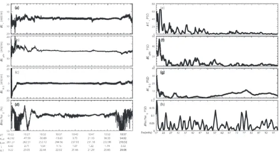
As reported by Ouyang et al. (2018), ULF oscillations of electricfield observed by the DEMETER satellite mostly occur on the nightside. According to latitudes where these nightside ULF oscillations occur, we may categorize them into three main types. Thefirst two types mainly occur at middle and low latitudes (L < 2) and are defined in Ouyang et al. (2018). Types I and II are respectively defined as electric field oscilla-tions with and without simultaneously significant electron density perturbaoscilla-tions, both types being classified as nonmagnetospheric ULF waves according to Ouyang et al. (2018). In addition, many electricfield oscilla-tions in the ULF range frequently occur at higher latitudes. Still, another possibility is that a minority of weaker oscillations also occur at middle and low latitudes but are not included in Types I and II. To simplify various ULF waves in the ionosphere, we categorize all ULF oscillations not classified into Types I and II as Type III. Figure 1 shows an example of Type III ULF oscillations, with the left plot (Figures 1a–1d) showing variations ofδEr,δEphi,δEB0, andδNe/Ne0along a half orbit on 6 March 2009, and the right plot (Figures 1e– 1h) presents the power spectral density (PSD) ofδEr,δEphi,δEB0, andδNe/Ne0in the L > 2 region corre-sponding to Figures 1a–1d. There are clear oscillations in δErandδEphicomponents (Figures 1a and 1b) around 10:22 to 10:31 UT, and electron density (Ne, Figure 1d) also shows large‐amplitude variations at higher latitudes, which are not similar to Ne perturbations associated with Type I. For Type I, the PSD of δNe/Ne0in the L < 2 region is similar to that of theδErandδEphicomponents (see Figure 1c in Ouyang et al., 2018). By contrast, Figures 1e–1h show that the PSD of the δErandδEphicomponents are similar but the PSD ofδNe/Ne0is different. In this study, to investigate the main types of ULF waves in the ionosphere, we use an automatic wave detection algorithm to obtain all wave events, and a detailed description of the algorithm is in section 2.3.
2.3. ULF Wave Detection Methodology
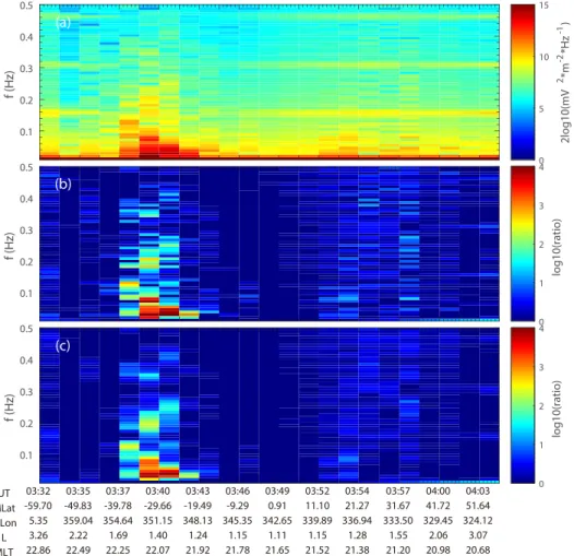
In this paper, we follow the automatic wave detection algorithm developed by Bortnik et al. (2007), which can automatically identify and characterize waves in afield‐aligned coordinate system. First, we conduct fast Fourier transform on the three electricfield components during consecutive and overlapped time segments. Each segment lasts ~2 min, with a 30% overlapping between the adjacent segments, and a Hamming window is used to reduce the edge effects. Since each sample array of the electricfield data includes 256 data points, there are 18 sample arrays during a 2‐min interval. The actual sampling interval duration is Ts= 256 × 18/ 39.0625≈ 118 s, so the consequent frequency resolution is fres= 39.0625/(39.0625 × 118) = 8.5 mHz. Second, we define the covariance matrix in the frequency domain and sum the square of off‐diagonal elements to obtain the total cross‐covariance power among the three components, which is labeled as Ci(f) at the specific time segment i. Figure 2a shows the dynamic spectrogram of total cross‐covariance power along one half orbit on 9 January 2010. There are disturbances visible below ~0.4 Hz around 03:40 UT and surrounded by some background noise. The background noise, M(f), is defined as the median of each frequency compo-nent during all the time segments along one half orbit. It is also noted that there are three spectral lines with
f~ 0.16 Hz, which are thought to be artificial signals arising from electromagnetic interferences from some
spacecraft subsystems. Figure 2b shows the spectrogram with the background noise removed, that is log10 (Ci(f))− log10(M(f)), where the disturbances around 03:40 UT are much more distinguishable. It can also
be noticed that the disturbances show irregular variations of the signal intensity as a function of frequency. To get a smoother spectrogram and better reveal the peak frequency we have applied a moving average to the spectrogram in Figure 2b. The moving average window was chosen to be the width of three frequency components (~25.5 mHz). The results are shown in Figure 2c, where spectral peaks (disturbances) can be detected according to the given threshold. The threshold value was set to be 1 on the logarithm scale, to ensure that the detected disturbances are at least 1 order of magnitude higher than the background level.
The lower and upper cutoff frequencies are set to 8.5 and 500 mHz (as most disturbances are below 500 mHz), respectively, and the minimum width is set to 17 mHz to ensure that the spectral peak does not only occur at a single frequency. It is also required that disturbances continue for at least three time segments, and we allow two time segments at the most to be skipped when they are surrounded by distur-bances. For each spectral peak, we obtain the beginning frequency (fb), the ending frequency (fe), the max-imum frequency (fmax), and the width of the frequency band (fwidth= fe− fb). In each time segment, there may be one or several spectral peaks, which are saved in onefile related to one half orbit. It is also necessary to group different spectral peaks in adjacent time segments into individual wave events.
Figure 1. An example of ultralow frequency oscillations occurring at higher latitudes along a half orbit on the nightside on
6 March 2009. (a–d) Detrended electric field components (δEr,δEphi, andδEB0) and relative disturbances of electron density (δNe/Ne0);δEr,δEphi,δEB0, andδNe are obtained by subtracting a moving average over ~200 s. (e–h) Power spectral density (PSD) ofδEr,δEphi,δEB0, andδNe/Ne0in the L > 2 region corresponding to (a–d).
We checked spectral peaks for continuity by using the Boolean conditions as given in Bortnik et al. (2007). Our procedure would traverse every peak from the lower frequency to the higher frequency in the time seg-ment i to check the continuity with every peak in the time segseg-ment i + 1 or i + j, where j must be less than 3, which means that two time segments at the most can be skipped (for example, due to noise, beating, and amplitude modulation). If there is continuity between two peaks, they would be given the same tag and trea-ted as part of the same wave event. After the whole continuity check processfinishes, each spectral peak receives an attached tag. We can group the associated peaks and save them into an individual wave eventfile according to the same tag.
2.4. Statistical Survey of Nightside ULF Waves in the Ionosphere
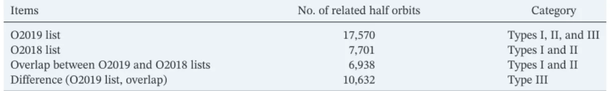
The ULF wave detection methodology is applied to all electricfield data on the nightside for 24,378 half orbits during ~5.5 years and obtained 41,343 wave events related to 17,570 half orbits in total (referred to in the following as the O2019 list). We assume that the O2019 list includes all main types of ULF waves, that is, Types I, II, and III. On the other hand, there are 7,701 half orbits with significant ULF oscillations in ~5.5 years identified by the selection criteria of Types I and II events in Ouyang et al. (2018), labeled in the following as the O2018 list. Comparing the O2019 list with the O2018 list, it is found that the overlap between these two lists is 6,938 half orbits. The difference between the O2019 list and events related to these 6,938 half orbits constitutes the Type III events, the determination of their origin, magnetospheric or non-magnetospheric, being the objective of the present study. Table 1 presents a brief summary of the relation-ship between O2019 and O2018 lists.
Figure 2. An example of a dynamic spectrogram of total cross‐covariance power along a half orbit on the nightside on 9
January 2010. (a) Original dynamic spectra, (b) spectra with the background noise removed, and (c) moving average spectra.
Figure 3 shows the occurrence rate of these three types of events as a function of magnetic latitude and month. The occurrence rate is defined as the ratio of the number of ULF disturbance samples to the total number of half orbits in each bin. The results of the nonmagnetospheric category, Types I and II, are pre-sented in Figures 3a and 3b. One point that should be clarified is that Types I and II are defined as ULF oscil-lations in L < 2 (~|Mlat| < 45°) region, but Figures 3a and 3b show ULF wave occurrence along the entire half orbit. Thus, the event occurrence probability in ~|Mlat| > 45° region in Figures 3a and 3b will not be ana-lyzed. Types I and II wave events have a clear seasonal dependence with increased occurrence rates in the local summer in the Northern Hemisphere (in the following referred to as NH) and in both local winter and summer in the Southern Hemisphere (SH). This characteristic also suggests that these waves are not of magnetospheric origin, and a detailed discussion about the nonmagnetospheric origin of Types I and II is given in Ouyang et al. (2018). Figure 3c shows that the occurrence of Type III events maximizes close to equinoxes (March and April, and September and October), this being particularly visible at high latitudes in the SH and low latitudes in the NH. It is known that auroral activity also maximizes in such periods,
Table 1
Relationship Between O2019 and O2018 Lists
Items No. of related half orbits Category
O2019 list 17,570 Types I, II, and III
O2018 list 7,701 Types I and II
Overlap between O2019 and O2018 lists 6,938 Types I and II
Difference (O2019 list, overlap) 10,632 Type III
Figure 3. The occurrence rate of ultralow frequency (ULF) waves versus magnetic latitude (5° bins) in every month on the
nightside from May 2005 to November 2010. (a) Type I and (b) Type II, likely not magnetospheric ULF waves, and (c) Type III events, more likely related to magnetospheric ULF waves.
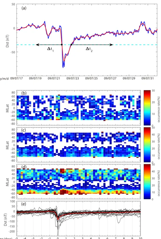
Figure 4. (a) An example of an isolated storm. The dashed cyan line indicates the quiet threshold value (−35 nT in this
case), which has two intersections (black dots) with the smoothed Dst time serials (red line). Based on these two inter-sections, Dst value must be larger than the quiet threshold value during the periodsΔt1(at least≥3 days) and Δt2(at least
≥5 days). (b–e) Superposed epoch analysis of ultralow frequency waves relative to geomagnetic storms. The occurrence rate of ultralow frequency waves is organized in bins of 6‐hr by 5° magnetic latitude for the nonmagnetospheric category: (b) Type I, (c) Type II, and (d) Type III wave events. The white means that there are no data in bins. (e) Dst values for 23 isolated storms (black lines) and the mean Dst value of 23 isolated storms (red line).
and these features suggest that the Type III events are more likely associated with magnetospheric ULF waves. To further study the dif-ferences between the sources of Types I and II on one side and Type III events on the other side, a superposed epoch analysis has been per-formed to compare their response to geomagnetic storms and is described in section 3.
3. Characteristics of ULF Wave Types During
Geomagnetic Storms
3.1. Storm Identification
To study“clean” storm effects, we use the Dst index to select isolated geomagnetic storms that must have a quiet period surrounding the minimum Dst. This selection algorithm is adapted from Bortnik et al. (2008). Periods with Dst <−50 nT are selected from the Dst data set during the ~5.5 years corresponding to our DEMETER data set. Wefirst find out all the dates with Dst (hour values) < −50 nT, and then locate the dates when they are not consecutive. Different periods with Dst <−50 nT can be identified by the nonconsecutive dates. For each period, we obtain the minimum Dst (Dstmin) and then set the quiet threshold value as the minimum of either 0.35 * Dstmin or −35 nT to ensure superstorms (Dst < −100 nT) to have lower quiet thresholds. Figure 4a illustrates an isolated geomagnetic storm. The blue line indicates the original Dst value, and the red line shows a 9‐hr moving average of the blue one. According to the Dstmin, the quiet threshold is obtained, shown as the cyan line, and two intersec-tions between the red line and the cyan line define the starting point of the preceding period Δt1and the suc-ceeding periodΔt2. If the Dst value is larger than the quiet threshold for the entire length ofΔt1(≥3 days) and Δt2(≥5 days), the storm is selected for our analysis. We selected 23 isolated storms through the above meth-odology from May 2005 to November 2010 (see Table 2 for details of these storms).
3.2. Superposed Epoch Analysis
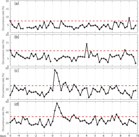
To study the temporal evolution of ULF wave activity in the ionosphere related to these isolated storms, we performed a superposed epoch analysis as shown in Figures 4b–4e. The time of each ULF disturbance rela-tive to the time of the Dstmin(t0) are calculated, and these disturbance samples of wave events are organized into bins of 5° magnetic latitude by 6‐hr relative time. The size of time bins is chosen after several trials to ensure it can tellfine details of temporal variation of ULF wave activity. In other words, it has to reach a com-promise between time resolution and sample numbers. Similar to Figure 3, the occurrence rate in each bin is shown in Figures 4b–4d. The results of nonmagnetospheric, Types I and II, wave events (L < 2, ~|Mlat| < 45°) shown in Figures 4b and 4c do not exhibit a close correspondence with the evolution of Dst values. A quan-titative analysis of Types I and II occurrence rate in the L < 2 region is presented in Figures 5a and 5b, show-ing that there is no significant enhancement of occurrence rate after t0. On the contrary, the occurrence rate of Type III wave events shown in Figure 4d correlates well with the temporal evolution of Dst values. A sharp change occurs around t0with weak occurrence before and enhanced occurrence after t0. It is known from Figure 4d that occurrence rate increases significantly both in southern and northern latitudes 6‐hr after t0, with the largest occurrence rate occurring within ~1 day after t0. The response time of ULF wave occurrence, about 6‐hr after t0, indicates a clear relationship between ULF waves and the recovery phase of geomagnetic storms. From the occurrence rate between 45° and 60° in NH and SH respectively shown in Figures 5c and 5d, significant enhanced occurrence rates last for less than 1 day in the northern latitudes and 1 day in the southern latitudes.
4. Discussion
The results presented above clearly show a different behavior of the two groups of ULF waves, the “nonmag-netospheric” ULF waves and Type III waves, with respect to their global distribution, seasonal dependence,
Table 2
The List of Isolated Storms
Number Time (UT) Dstmin(nT)
1 May 15, 2005 0800 −247 2 May 30, 2005 1300 −113 3 Jun 13, 2005 0000 −106 4 Jun 23, 2005 1000 −85 5 Jul 18, 2005 0600 −67 6 Aug 24, 2005 1100 −184 7 Oct 31, 2005 2000 −74 8 Jan 26, 2006 0300 −51 9 Mar 07, 2006 0100 −52 10 Sep 24, 2006 0900 −55 11 Oct 01, 2006 0500 −51 12 Nov 30, 2006 1300 −74 13 Dec 15, 2006 0700 −162 14 Mar 24, 2007 0800 −72 15 May 23, 2007 1300 −58 16 Oct 25, 2007 2100 −53 17 Nov 20, 2007 2000 −59 18 Mar 09, 2008 0500 −86 19 Jul 22, 2009 0600 −83 20 Feb 15, 2010 2300 −59 21 May 02, 2010 1800 −71 22 Aug 04, 2010 1900 −74 23 Oct 11, 2010 1900 −75
and their response to geomagnetic storms. The latter group occurs almost throughout the year, with higher occurrence rate at higher latitudes, and shows a clear correlation with storms. All these characteristics are in sharp contrast with those of nonmagnetospheric wave events, which show seasonal variations and no relation with storms. These marked differences indicate that the two groups of ULF wave events are truly distinct, which leads us to recognize Type III waves as most likely waves of magnetospheric origin. Past studies dealing with interhemispheric asymmetries of ULF waves have focused on ULF wave power obtained from ground‐based magnetometers located at conjugate locations from cusp latitudes to low lati-tudes. The discussed influence factors include local precipitation of electrons (Posch et al., 1999), ionospheric conductivity (Obana et al., 2005; Surkan & Lanzerotti, 1974), and the state of the ionosphere (Zesta et al., 2016). In contrast to single‐point observations made with ground‐based magnetometers, low Earth‐orbiting satellites offer the capability of an extensive survey over the full range of longitudes and latitudes. In this study, we have obtained a global view of interhemispheric asymmetries in ULF wave occurrence based on DEMETER satellite observations. In addition, interhemispheric asymmetry in response to geomagnetic storms in the topside ionosphere has been reported in total electron content and electron density (Astafyeva et al., 2015; Yizengaw et al., 2006).
Our study of ULF waves is based on electricfield measurements in the topside ionosphere. The total iono-spheric electricfield includes the electric field in the incident and reflected waves, which is primarily depen-dent on the ionospheric conductivity (Southwood & Hughes, 1983). When the ionospheric conductivity is high, good reflection occurs (Hughes & Southwood, 1976b). In this circumstance, most of incident waves are reflected and the electric field of reflected waves roughly cancels the electric field of incident waves.
Figure 5. Quantitative analysis of occurrence rate relative to geomagnetic storms based on Figures 4b–4d. (a, b) Averaged
occurrence rate of Types I and II wave events between−45° and 45° Mlat, corresponding to results in Figures 4b and 4c. (c) Averaged occurrence rate of Type III wave events between 45° and 60° Mlat. (d) Similar to (c) but between−45° and −60° Mlat. Red lines show thresholds of occurrence rate, which are defined as the mean plus double standard deviations of occurrence rate before t0(−5 to 0 days) in the respective situations.
Thus, the total ionospheric electricfield is small. Our results are observed at nighttime, when the ionospheric conductivity is generally low, leading to less reflection, and thus, the total electric field in the ionosphere is relatively large. Figure 3c shows a higher occurrence rate of ULF waves between−45° and −65°, hence larger electricfield fluctuations in this latitude band in the SH at nighttime.
Similarly, Figure 4d also shows a stronger occurrence rate of ULF waves in response to geomagnetic storms in the SH. However, among the isolated storms (see Table 2), 10 storms occur during the NH summer (May to August),five during the SH summer (November to February), and eight during equi-noxes (March, April, September, and October). Storms in NH summer are thus twice as numerous as those in SH summer. Ionospheric conductivity is larger in the summer hemisphere, which may lead to a good reflection of ULF waves with consequently small total electric field in the ionosphere. To check
Figure 6. Superposed epoch analysis of ultralow frequency (ULF) waves relative to geomagnetic storms occurred in different seasons. The occurrence rate of ULF
waves is organized in bins of 6‐hr by 5° magnetic latitude. (a–d) Superposed epoch analysis of ULF waves relative to geomagnetic storms that occurred in the Northern Hemisphere summer, (a) Type I, (b) Type II, (c) Type III, and (d) Dst values (black lines) and the mean Dst (red line) of 10 storms in the Northern Hemisphere summer. (e–h) Similar to (a–d), results for five storms in the Southern Hemisphere summer. (i–l) Similar to (a–d), results for eight storms during equinoxes.
whether the interhemispheric asymmetry in Figure 4d results from the seasonal effect, we separate these storms according to seasons to conduct superposed epoch analyses as shown in Figure 6. It is found that results of storms during the NH summer (Figure 6c) show enhanced ULF wave occurrence rates in the SH, with little or no significantly enhanced occurrence in the NH. Due to limited samples, the results of storms during the SH summer (Figure 6g) show a scattered distribution of ULF wave occurrence rates, but it still presents higher ULF wave occurrence rates in the NH and lower rates in the SH. For storms during equinoxes (Figure 6k), results show a weak interhemispheric asymmetry with a preference of ULF wave occurrence for the SH. Thus, taking apart the seasonal effect, these last results might still indicate the interhemispheric asymmetry of ionospheric conductivity at nighttime with generally larger conductiv-ities (hence denser ionosphere) in the NH. However, with a small size of storms during the SH summer and around equinoxes, caution must be applied, as the results of storms during the SH summer only show a low occurrence rate in the SH and results of storms around equinoxes show a minor asymmetry with a preference for the SH.
5. Conclusions
In this paper, we use ULF waves identified by an automatic detection algorithm to study their features in the ionosphere using electricfield data in the DC/ULF range observed by the DEMETER satellite in the period from May 2005 to November 2010. Compared to previous studies of ULF waves in the ionosphere, this study is unique and led to the following conclusions:
1. The characteristics of nonmagnetospheric and magnetospheric ULF waves in the ionosphere are revealed with the aid of a superposed epoch analysis. The nonmagnetospehric ULF wave events show seasonal variations with a higher occurrence rate in the winter and summer but do not exhibit response to geomag-netic storms. Type III ULF waves occur almost throughout the year with a noticeable enhancement around equinoxes especially in the SH and mostly concentrate in a narrower latitude band from−45° to−65°. Furthermore, their occurrence rates have a very clear correspondence with the recovery phase of geomagnetic storms. More likely these waves originated from magnetospheric processes.
2. Magnetospheric ULF waves in the ionosphere, particularly around storms, show an interhemispheric asymmetry with a higher occurrence rate in the SH. This asymmetry can be partly explained by the fact that more of the analyzed storms occurred during NH summer and hence higher plasma densities and conductivities in the NH. However, the investigation of few storms that occurred around equinoxes also indicates a minor asymmetry. Thus, the ionospheric conductivity at nighttime in the SH could be lower than in the NH.
References
Allan, W., & Poulter, E. M. (1992). ULF waves‐their relationship to the structure of the Earth's magnetosphere. Reports on Progress in
Physics, 55(5), 533.
Astafyeva, E., Zakharenkova, I., & Doornbos, E. (2015). Opposite hemispheric asymmetries during the ionospheric storm of 29–31 August 2004. Journal of Geophysical Research: Space Physics, 120, 697–714. https://doi.org/10.1002/2014JA020710
Berthelier, J. J., Godefroy, M., Leblanc, F., Malingre, M., Menvielle, M., Lagoutte, D., et al. (2006). ICE, the electricfield experiment on DEMETER. Planetary and Space Science, 54(5), 456–471. https://doi.org/10.1016/j.pss.2005.10.016
Bortnik, J., Cutler, J., Dunson, C., & Bleier, T. (2007). An automatic wave detection algorithm applied to Pc1 pulsations. Journal of
Geophysical Research, 112, A04204. https://doi.org/10.1029/2006JA011900
Bortnik, J., Cutler, J., Dunson, C., Bleier, T., & McPherron, R. (2008). Characteristics of low‐latitude Pc1 pulsations during geomagnetic storms. Journal of Geophysical Research, 113, A04201. https://doi.org/10.1029/2007JA012867
Fraser‐Smith, A. C. (1993). ULF magnetic fields generated by electrical storms and their significance to geomagnetic pulsation generation.
Geophysical Research Letters, 20(6), 467–470. https://doi.org/10.1029/93GL00087
Fraser‐Smith, A. C., & Kjono, S. N. (2014). The ULF magnetic fields generated by thunderstorms: A source of ULF geomagnetic pulsations?
Radio Science, 49, 1162–1170. https://doi.org/10.1002/2014RS005566
Hughes, W. J. (1974). The effect of the atmosphere and ionosphere on long period magnetospheric micropulsations. Planetary and Space
Science, 22(8), 1157–1172. https://doi.org/10.1016/0032‐0633(74)90001‐4
Hughes, W. J., & Southwood, D. J. (1976a). An illustration of modification of geomagnetic pulsation structure by the ionosphere. Journal of
Geophysical Research, 81(19), 3241–3247. https://doi.org/10.1029/JA081i019p03241
Hughes, W. J., & Southwood, D. J. (1976b). The screening of micropulsation signals by the atmosphere and ionosphere. Journal of
Geophysical Research, 81(19), 3234–3240. https://doi.org/10.1029/JA081i019p03234
Iyemori, T., Nakanishi, K., Aoyama, T., Yokoyama, Y., Koyama, Y., & Lühr, H. (2015). Confirmation of existence of the small‐scale field‐ aligned currents in middle and low latitudes and an estimate of time scale of their temporal variation. Geophysical Research Letters, 42, 22–28. https://doi.org/10.1002/2014GL062555
Lagoutte, D., Brochot, J. Y., & Carvalho, D. (2006). DEMETER microsatellite scientific mission center data product description. Demeter. Acknowledgments
This work was supported by the National Key R&D Program of China (2018YFC1503506), NSFC Grants (41404126 and 41574139), APSCO Earthquake Research Project Phase II, and the Civil Aerospace Research Project (ZH‐1‐DMYZ‐01). The authors thank the DEMETER scientific mission center for the high‐quality data, which can be accessed at https://cdpp‐archive. cnes.fr/. We are grateful to Chao Xiong, Chen Zhou, Libo Liu, and Huijun Le for helpful discussions.
Lühr, H., Maus, S., Rother, M., & Cooke, D. (2002). First in‐situ observation of night‐time F region currents with the CHAMP satellite.
Geophysical Research Letters, 29(10), 1489. https://doi.org/10.1029/2001GL013845
Mazur, N. G., Fedorov, E. N., Pilipenko, V. A., & Vakhnina, V. V. (2018). ULF electromagneticfield in the upper ionosphere excited by lightning. Journal of Geophysical Research: Space Physics, 123, 6692–6702. https://doi.org/10.1029/2018JA025622
McPherron, R. (2005). Magnetic pulsations: Their sources and relation to solar wind and geomagnetic activity. Surveys in Geophysics, 26(5), 545–592. https://doi.org/10.1007/s10712‐005‐1758‐7
Nakanishi, K., Iyemori, T., Taira, K., & Lühr, H. (2014). Global and frequent appearance of small spatial scalefield‐aligned currents possibly driven by the lower atmospheric phenomena as observed by the CHAMP satellite in middle and low latitudes. Earth, Planets and Space,
66(1), 40. https://doi.org/10.1186/1880‐5981‐66‐40
Obana, Y., Yoshikawa, A., Olson, J. V., Morris, R. J., Fraser, B. J., & Yumoto, K. (2005). North‐south asymmetry of the amplitude of high‐ latitude Pc 3–5 pulsations: Observations at conjugate stations. Journal of Geophysical Research, 110, A10214. https://doi.org/10.1029/ 2003JA010242
Ouyang, X. Y., Zong, Q. G., Bortnik, J., Wang, Y. F., Chi, P. J., Zhou, X. Z., et al. (2018). Nightside ULF waves observed in the topside ionosphere by the DEMETER satellite. Journal of Geophysical Research: Space Physics, 123, 7726–7739. https://doi.org/10.1029/ 2018JA025248
Pilipenko, V., & Heilig, B. (2016). ULF waves and transients in the topside ionosphere. In A. Keiling, D. Lee, & V. Nakariakov (Eds.), Low‐
frequency waves in space plasmas(pp. 15–29). https://doi.org/10.1002/9781119055006.ch2
Posch, J. L., Engebretson, M. J., Weatherwax, A. T., Detrick, D. L., Hughes, W. J., & Maclennan, C. G. (1999). Characteristics of broadband ULF magnetic pulsations at conjugate cusp latitude stations. Journal of Geophysical Research, 104(A1), 311–331. https://doi.org/10.1029/ 98JA02722
Southwood, D., & Hughes, W. (1983). Theory of hydromagnetic waves in the magnetosphere. Space Science Reviews, 35(4), 301–366. Stolle, C., Lühr, H., Rother, M., & Balasis, G. (2006). Magnetic signatures of equatorial spread F as observed by the CHAMP satellite. Journal
of Geophysical Research, 111, A02304. https://doi.org/10.1029/2005JA011184
Surkan, A. J., & Lanzerotti, L. J. (1974). ULF geomagnetic power near L=4 3. Statistical study of power spectra in conjugate areas during December solstice. Journal of Geophysical Research, 79(16), 2403–2412. https://doi.org/10.1029/JA079i016p02403
Yizengaw, E., Moldwin, M. B., Komjathy, A., & Mannucci, A. J. (2006). Unusual topside ionospheric density response to the November 2003 superstorm. Journal of Geophysical Research, 111, A02308. https://doi.org/10.1029/2005JA011433
Zesta, E., Boudouridis, A., Weygand, J. M., Yizengaw, E., Moldwin, M. B., & Chi, P. (2016). Interhemispheric asymmetries in magneto-spheric energy input. In T. Fuller‐Rowell, E. Yizengaw, P. H. Doherty, & S. Basu (Eds.), Ionomagneto-spheric space weather (pp. 3–20). John Wiley & Sons, Inc. https://doi.org/10.1002/9781118929216.ch1