Marine productivity response to Heinrich events: a model-data comparison

HAL Id: hal-02931502

https://hal.archives-ouvertes.fr/hal-02931502

Submitted on 9 Oct 2020

HAL is a multi-disciplinary open access

archive for the deposit and dissemination of

sci-entific research documents, whether they are

pub-lished or not. The documents may come from

teaching and research institutions in France or

abroad, or from public or private research centers.

L’archive ouverte pluridisciplinaire HAL, est

destinée au dépôt et à la diffusion de documents

scientifiques de niveau recherche, publiés ou non,

émanant des établissements d’enseignement et de

recherche français ou étrangers, des laboratoires

publics ou privés.

Marine productivity response to Heinrich events: a

model-data comparison

V. Mariotti, L. Bopp, A. Tagliabue, M. Kageyama, D. Swingedouw

To cite this version:

V. Mariotti, L. Bopp, A. Tagliabue, M. Kageyama, D. Swingedouw. Marine productivity response to

Heinrich events: a model-data comparison. Climate of the Past, European Geosciences Union (EGU),

2012, 8 (5), pp.1581-1598. �10.5194/cp-8-1581-2012�. �hal-02931502�

www.clim-past.net/8/1581/2012/ doi:10.5194/cp-8-1581-2012

© Author(s) 2012. CC Attribution 3.0 License.

Climate

of the Past

Marine productivity response to Heinrich events:

a model-data comparison

V. Mariotti1, L. Bopp1, A. Tagliabue1,2,3, M. Kageyama1, and D. Swingedouw1

1_{Laboratoire des Sciences du Climat et de l’Environnement, UMR8212,}

IPSL-CEA-CNRS-UVSQ – Centre d’Etudes de Saclay, Orme des Merisiers bat. 701, 91191 Gif Sur Yvette, France

2_{Dept. of Oceanography, Upper Campus, University of Cape Town, Cape Town, 7701, South Africa}

3_{Southern Ocean Climate and Carbon Observatory, CSIR, Stellenbosch, 7599, South Africa}

Correspondence to: V. Mariotti (veronique.mariotti@lsce.ipsl.fr)

Received: 26 January 2012 – Published in Clim. Past Discuss.: 14 February 2012 Revised: 31 July 2012 – Accepted: 9 September 2012 – Published: 16 October 2012

Abstract. Marine sediments records suggest large changes in marine productivity during glacial periods, with abrupt vari-ations especially during the Heinrich events. Here, we study the response of marine biogeochemistry to such an event by using a biogeochemical model of the global ocean (PISCES) coupled to an ocean-atmosphere general circulation model (IPSL-CM4). We conduct a 400-yr-long transient simulation under glacial climate conditions with a freshwater forcing of 0.1 Sv applied to the North Atlantic to mimic a Hein-rich event, alongside a glacial control simulation. To eval-uate our numerical results, we have compiled the available marine productivity records covering Heinrich events. We find that simulated primary productivity and organic carbon export decrease globally (by 16 % for both) during a Hein-rich event, albeit with large regional variations. In our ex-periments, the North Atlantic displays a significant decrease, whereas the Southern Ocean shows an increase, in agreement with paleo-productivity reconstructions. In the Equatorial Pa-cific, the model simulates an increase in organic matter ex-port production but decreased biogenic silica exex-port. This an-tagonistic behaviour results from changes in relative uptake of carbon and silicic acid by diatoms. Reasonable agreement between model and data for the large-scale response to Hein-rich events gives confidence in models used to predict fu-ture centennial changes in marine production. In addition, our model allows us to investigate the mechanisms behind the observed changes in the response to Heinrich events.

1 Introduction

Marine primary productivity (PP) is a key component of climate-active biogeochemical cycles such as the carbon cy-cle. It also sustains upper trophic levels and marine resources (Pauly and Christensen, 1995) and is the first level of marine food web impacted by climate change. The response of PP to future climate change is largely uncertain (e.g. Taucher and Oschlies, 2011) and natural variability hampers the detec-tion of unequivocal trends from the 15-yr ocean colour satel-lite record (Henson et al., 2010). Coupled climate – marine biogeochemical models are used to simulate the evolution of marine PP over the historical period and under future sce-narios. Four models (Steinacher et al., 2010) show a global decrease in PP and in the export production of organic car-bon at the base of the euphotic layer (EXP) to deeper waters of between 2 and 20 % by 2100, relative to preindustrial con-ditions, notwithstanding regional variability in the response. A reduced input of nutrients to the euphotic zone from sub-surface waters due to increased stratification decreases PP in the North Atlantic and tropical regions, whereas lower light limitation increases Southern Ocean PP (Bopp et al., 2001; Steinacher et al., 2010). Another model (Schmittner et al., 2008) shows an increase in PP and a decrease in EXP due to enhanced remineralisation in response to increas-ing temperature. Nevertheless, evaluation of these models on such decadal-to-centennial time scales is still difficult due to sparse data covering these time scales (Schneider et al., 2008) and relatively moderate climatic change.

1582 V. Mariotti et al.: Marine productivity response to Heinrich events Turning to the geologic past, the last 70 000 yr of

paleo-records may permit the evaluation of such climate-marine biogeochemical models on centennial time scales. These records show large and rapid variations linked to abrupt events such as Heinrich events (HEs) (Heinrich, 1988). During these events, massive iceberg discharges occur in the North Atlantic Ocean (Broecker et al., 1992), affect-ing the global ocean circulation through a collapse of the Atlantic meridional overturning circulation (AMOC) (Mc-Manus et al., 2004). At the same time, there is a cooling over the North Atlantic Ocean both seen in data (Voelker, 2002; Bard et al., 2000; Cacho et al., 1999) and reproduced in cli-mate model experiments (Kageyama et al., 2010; Swinge-douw et al., 2009; Ganopolski and Rahmstorf, 2001). Along-side the climate and ocean circulation changes, there is ample evidence of abrupt variations in biogeochemical variables.

From ice cores, we know that atmospheric N2O

concentra-tions decreased during HEs (Fl¨uckiger et al., 2004; Stocker and Schilt, 2008). Schmittner and Galbraith (2008) explain this decrease by a global reduction in primary productiv-ity, especially in the Indo-Pacific region, which induces in-creased subsurface oxygen concentrations and then reduced

N2O production. We can also find biogeochemical variations

such as EXP variations in marine sediments (e.g. Anderson et al., 2009; Nave et al., 2007). While marine paleo-records give a picture of regional processes during HEs, such as a de-crease in North Atlantic EXP and an inde-crease in the Southern Ocean, they cannot give an integrated view of the global re-sponse of marine biogeochemistry to such events due to their sparse distribution.

Biogeochemical models can provide information concern-ing centennial-scale marine carbon cycle dynamics. Un-til now, most “paleo” setting studies aimed at

understand-ing glacial–interglacial variations of atmospheric pCO2

ob-served in ice core data (Monnin et al., 2001). To explain the

lower pCO2 during glacial times compared to interglacial

times, different mechanisms have been investigated, such as Southern Hemisphere westerly-wind modification (Tog-gweiler et al., 2006), sinking of brines (Bouttes et al., 2010), marine biology enhancement through iron fertilisation (Bopp et al., 2003) or larger nutrient availability (Matsumoto et al.,

2002). Alongside past CO2 concentrations, recent models

have also been used to understand changes in marine pro-ductivity between glacial and interglacial times (Kageyama et al., 2012; Oka et al., 2011; Tagliabue et al., 2009; Bopp et al., 2003). In agreement with the marine productivity com-pilation of Kohfeld et al. (2005), they all find a dipole effect in the Southern Ocean with enhanced EXP in the middle lat-itudes due to increased iron deposition and decreased EXP in the high latitudes due to increased light limitation following enhanced glacial sea-ice. The response in the other regions of the ocean are model dependent

Nonetheless, on submillennial time scales, three model studies using Earth system models of intermediate com-plexity (EMICs) (Schmittner, 2005; Menviel et al., 2008;

Schmittner and Galbraith, 2008) and two model studies using atmosphere-ocean general circulation models (AOGCMs) (Obata, 2007; Bozbiyik et al., 2011) have investigated the response of marine biogeochemistry to Heinrich-like events. Schmittner (2005), Obata (2007) and Bozbiyik et al. (2011) studies have been performed under preindustrial background climate, but as seen in Menviel et al. (2008) the structure of the marine productivity changes obtained under prein-dustrial and LGM conditions is fairly similar, so they can be compared to marine records of HEs. Bozbiyik et al. (2011) do not show changes in EXP, but the other studies do. They all simulate a global decrease of marine produc-tivity and a common response in certain regions (North At-lantic Ocean, Benguela coast, Mauritanian coast) matching the data, whereas in other regions they do not agree with the marine response seen in data (Eastern Equatorial Pa-cific, Southern Ocean, see Table 1). These regional differ-ences between model results and marine sediment records suggest that physical or biogeochemical processes might be missing or underestimated in these models. Such model-data mismatches need to be investigated further to understand the main mechanisms controlling key ocean regions.

Moreover, in the future, the Greenland ice sheet may melt, releasing an amount of freshwater that might resemble a HE, albeit smaller and released more to the North. The impact of such a release on the AMOC and marine biogeochemistry implies different opposing mechanisms with large uncertain-tities (Swingedouw et al., 2007). Validating climate models with marine biogeochemistry data from the past is clearly a key to properly evaluate the response of marine system to fu-ture freshwater input. Importantly, it is still rare that identical marine biogeochemical models are employed and tested in “paleo” settings, as well as being used for predictions of our future climate.

In this study, we investigate the global and regional re-sponse of marine biogeochemistry to a Heinrich-like event with the state of the art biogeochemical model PISCES, which has also been used for future climate projections (Steinacher et al., 2010). In a first section we present the data compilation gathered, the experimental design and the comparison method performed between model and data. Then a second section details the results of the simulations both globally and regionally. A third section both discusses the discrepancies between our results and previous model studies and give some insights on potential effect of future Greenland ice sheet melting on marine biology.

2 Data compilation, model and experimental design 2.1 Data compilation

In order to evaluate our numerical results, we have compiled existing marine sediment cores documenting millennial-scale paleoproductivity changes during the past 70 000 yr.

T able 1. Data compilation of paleoproducti vity changes in response to Heinrich ev ents (HEs). F or each record and each ev ent, we summarise the trend of the proxies for paleoproducti vity by a certain number of “ − ” or “+” signs. Each “ − ” (resp. “+”) corresponds to a sensor indicating a sig nificant decrease (resp. increase) in EXP . W e discriminate between significant and not significant trend in sensors by applying a simple test on eac h time series. W e compare the trend of the first 500 yr follo wing a dated HE to the mean and v ariance of the 300 0 yr preceding this dated HE (resp. 2000 yr for the Y ounger Dryas (YD)). If the v alue of the first 500 yr is hig her (resp. lo wer) than the additio n of the mean and the v ariance (resp. the dif ference between the mean and the v ariance) of the la st 3 000 yr , we consider it as a signific ant increase (resp. decrease). When there is not such a significant trend, we display an “x”. Some records, while ha ving a suf ficient time resolution (less than 500 yr between tw o measurements), had no dated HEs or YD. W ould we ha v e discarded them, only 52 o ut of the 74 studies w ould ha v e remained. W e decided to k eep them and to date the HEs and YD ourselv es on the time series, taking as an onset for these ev ents − 13 k yr for YD, − 18 k yr for HE1, − 26.5 k yr for H E2, − 32.7 k yr for HE 3, − 40.2 k yr for HE4, − 50 k yr for HE5 and − 63.2 k yr for HE6 (follo win g Sanchez Go ˜ni and Harrison (2010 )). As there are time dating error bars issues on paleo-data, we consider these results as exploratory h ypotheses, in the absence of a real timing for these ev ents. T o dif ferentiate them from the well dated results we added a “?” in front of the concerned results. F or each record, we summarise the results of all HEs and YD in one “v alue”: when we add all th e “–” and “+”, if we obtain one “–” (resp. “+”), we write one “–” (resp. “+”), if we obtain more than tw o “–” (resp. “+”), we write “--” (resp. “++”) and finally if we ha v e an equal number of “–” and “+” (or only “x”), we write an “x” because we consider that the records do es not gi v e a significant trend. Core Re gion Latitude Longitude W ater Producti vity YD HE1 HE2 HE3 HE4 HE5 HE6 Global References depth(m) indicators North Atlantic Ocean MD95-2008 – 62.74 − 3.99 1016 C /N, Cor g, diatoms x x x Na v e et al. (2007 ) EN AM33 N A TL 61.26 − 11.11 1217 foram s -x x x -x -Rasmussen et al. (2002 ) MD95-2014 N A TL 60.58 − 22.08 2397 C/N, Cor g, diatoms x -Na v e et al. (2007 ) DS97-2P N A TL 58.93 − 30.40 1685 foram s -x -Rasmussen et al. (2002 ) BOFS-14K N A TL 58.62 − 19.44 1759 ph y todetritus ?x ?x ?x ?x Thomas et al. (1995 ) SU90-16 N A TL 58.22 − 45.17 2100 C/N, Cor g, diatoms + -x Na v e et al. (2007 ) M23415 N A TL 53.18 − 19.15 2472 chlor in ?x x + x x x x + W einelt et al. (2003 ) SU90-39 N A TL 52.57 − 21.93 3955 C/N, Cor g, diatoms -x -Na v e et al. (2007 ) BOFS-5K N A TL 50.69 − 21.87 3547 ph y todetritus -Thomas et al. (1995 ) HU 91-045-094 N A TL 50.20 − 45.69 3448 Cor g , δ 13 C , dinoc ysts -Radi and de V ernal (2008 ) SU90-44 N A TL 50.02 − 17.10 4279 C/N, Cor g, diatoms x x x Na v e et al. (2007 ) M15612 N A TL 44.36 − 26.54 3050 foram s ?x x -x + + x Kiefer (1998 ) SU92-03 N A TL 43.20 − 10.11 3005 Pe xp (SIMMAX28 model) -x -Salgueiro et al. (2010 ) MD95-2027 N A TL 41.74 − 52.41 4112 C/N, Cor g, diatoms -Na v e et al. (2007 ) MD95-2040 N A TL 40.58 − 9.87 2465 P exp (SIMMAX28 model) x -x -V oelk er et al. (2009 ) MD95-2040 N A TL 40.58 − 9.87 2465 C aCO3, C37, Pe xp (SIMMAX28 model) x -x x x -P ailler and Bard (2002 ), Salgueiro et al. (2010 ) SU90-03 N A TL 40.05 − 32.00 2475 C/N, Cor g, diatoms x x x Na v e et al. (2007 ) MD95-2041 – 37.83 − 9.52 1123 P exp (SIMMAX28 model) -x -V oelk er et al. (2009 ) MD95-2042 N A TL 37.75 − 10.17 3146 CaCO 3, C37, Pe xp (SIMMAX28 model) x -x -x -P ailler and Bard (2002 ), Salgueiro et al. (2010 ) MD95-2043 N A TL 36.14 − 2.62 1841 C or g, Ba -x x -Moreno et al. (2004 ) MD99-2339 – 35.89 − 7.53 1170 P exp (SIMMAX28 model) x x x x V oelk er et al. (2009 ) MD04-2805 CQ MA U 34.51 − 7.02 859 δ 13 C + x x + Penaud et al. (2010 ) OCE326GGC6 N A TL 33.69 − 57.58 4541 diatom s x x x Gil et al. (2009 ) GeoB5546-2 MA U 27.53 − 13.73 1070 Cor g , dinoc ysts x + x x + x ++ Holzw arth et al. (2010 ) GeoB7926-2 MA U 20.22 − 18.45 2500 Cor g , opal, diatoms + x + Romero et al. (2008 ) GeoB9526-5 MA U 12.44 − 18.06 3231 Cor g ?x + + ++ Zarriess and Mack ensen (2010 ) GeoB9527-5 MA U 12.44 − 18.22 3671 Cor g ?-+ + ++ Zarriess and Mack ensen (2010 ) M35003-4 – 12.08 − 61.25 1299 Cor g , δ 13 C -x -V ink et al. (2001 ) PL07-39PC – 10.70 − 64.94 790 Cor g -?x -Dean (2007 ) PL07-57PC – 10.68 − 64.96 815 gre y scale + + Hughen et al. (1996 )

1584 V. Mariotti et al.: Marine productivity response to Heinrich events T able 1. Continued. Core Re gion Latitude Longitude W ater Producti vity YD HE1 HE2 HE3 HE4 HE5 HE6 Global References depth(m) indicators North P acific Ocean EW0408-85JC – 59.56 − 144.15 682 d iatoms, silicoflagellates -Barron et al. (2009 ) EW0408-66JC – 57.87 − 137.10 426 d iatoms, silicoflagellates -Barron et al. (2009 ) EW0408-11JC – 55.63 − 133.51 183 d iatoms, silicoflagellates + + + + Barron et al. (2009 ) MD02-2489 – 54.39 − 148.92 3640 C or g, opal, chlorins -Gebhardt et al. (2008 ) ODP Site 887 – 54.37 − 148.45 3647 B a/Al, opal ?+ ?-?x Galbraith et al. (2007 ) JPC17 – 53.93 178.70 2209 CaCO3, Ba, opal ?x ?x ?x Brunelle et al. (2010 ) MD01-2416 – 51.27 167.73 2317 Cor g, opal, chlorins x x x Gebhardt et al. (2008 ) ODP Site 882 – 50.35 167.58 3300 Ba/Al, opal ? -?x ? -Galbraith et al. (2007 ) GGC27 – 49.60 150.18 995 CaCO3, Ba, opal ?x ?x ?x Brunelle et al. (2010 ) PC13 – 48.72 168.30 2393 CaCO3, Ba, opal ?x ?x ?x Brunelle et al. (2010 ) W87-09-13PC – 42.12 − 125.75 2712 C or g, opal, δ₁₅ N ? -?+ ?-?x ? -?+ ? -Kienast et al. (2002 ) ODP Site 1019 – 41.68 − 124.93 980 C or g - ? -Dean (2007 ) MV99 GC31/PC10 – 23.47 − 111.60 700 C or g ?-?x ?-?x ?x ?x ? -Ortiz et al. (2004 ) MD02-2508 – 23.47 − 111.60 606 B r, forams x x x -x -Cartapanis et al. (2011 ) MD02-2519 – 22.51 − 106.65 955 C or g, opal ?x ?x ? -?x ? -Arellano-T orres et al. (2011 ) Core 17940-2 – 20.12 117.38 1727 Cd/Ca, opal x x x x x Lin et al. (1999 ) ODP Site 1144 – 20.05 117.42 2036 chlorin ?-?x ?x ?x ?x ?x ?x ?-Higginson et al. (2003 ) Core 17950-2 – 16.09 112.9 1865 Cd/Ca, opal x x + x + x ++ Lin et al. (1999 ) MD02-2524 – 12.01 − 87.91 863 Cor g , opal ?x ?x ?x ?x Arellano-T orres et al. (2011 ) MD02-2524 – 12.01 − 87.91 863 Cor g , opal -x -x -Piche vin et al. (2010 ) MD97-2141 – 8.80 121.30 3633 coccolithophores ?x ?x x x x x Dannenmann et al. (2003 ) MD02-2529 – 8.21 − 84.12 1619 opal, diatoms x x x x x -Romero et al. (2011 ) ODP Site 1242 – 7.86 − 83.61 1364 Cor g ?x ?x ?x ?x Martinez and Robinson (2010 ) Eastern Equatorial P acific Ocean ODP Site 1240 EEP 0.02 − 86.46 2921 Cor g , opal ?x ?x ?+ ?+ Piche vin et al. (2009 ) ODP Site 1240 EEP 0.02 − 86.46 2921 Cor g , opal ?x ?+ ?+ ?++ Arellano-T orres et al. (2011 ) ODP Site 1240 EEP 0.02 − 86.46 2921 alk eno nes, brassicasterol ?x ?-?+ + ?+ ?++ Calv o et al. (2011 ) ME0005A-24JC EEP 0.02 − 86.46 2941 Cor g + + Kienast et al. (2006 ) ME0005A-24JC EEP 0.02 − 86.46 2941 Cor g , opal, δ₁₅ N ++ ++ + ++ Dubois et al. (2011 ) South P acific Ocean GeoB7112-5 – − 24.03 − 70.82 2507 Cor g , opal ? - ? -Mohtadi and Hebbeln (2004 ) GeoB7139-2 – − 30.20 − 71.98 3267 Cor g , opal ?+ ?x ?-?x Mohtadi and Hebbeln (2004 ) GeoB3359-3 – − 35.22 − 72.81 678 Cor g , opal ?+ ?+ ?++ Romero et al. (2006 ) ODP Site 1233 – − 41.00 − 74.45 838 cocco lithophores + ?+ + Saa v edra-Pellitero et al. (2011 )

T able 1. Continued. Core Re gion Latitude Longitude W ater Producti vity YD HE1 HE2 HE3 HE4 HE5 HE6 Globa l References depth(m) indica tors South Atlantic Ocean GeoB3912-1 – − 3.67 − 37.72 767 Co rg x + x + x x x + + Jennerjahn et al. (2004 ) GeoB1706-2 BEN − 19.56 11.18 980 Cor g, opal, diatoms ?x ?x ?-?x ? -Romero (2010 ) GeoB1711-4 BEN − 23.32 12.38 1967 Cor g, opal, diatoms ?+ ? -Romero (2010 ) GeoB3606-1 BEN − 25.47 13.08 1785 Cor g, opal, diatoms ?x ?+ ?x ? - ? - ? -Romero (2010 ) Indian Ocean Core 136 KL IND 23.12 66.50 568 Cor g ?-?x ?x ?x ? -?x -Higginson et al. (2004 ) Core 136 KL IND 23.12 66.50 568 Cor g, C37 ? -Schulte and M ¨uller (2001 ) RC27-23 IND 17.99 57.59 820 chlorin, nitrogen ?x ?-?x ?x ?x ?x ?-Altabet et al. (2002 ) Core 905 IND 10.77 51.95 1586 Cor g, δ 15 N , Ba/Al -x -Iv anochk o et al. (2005 ) Southern Ocean MD97-2120 – − 45.53 1 74.93 1210 alk enones, brassicasterol + + x x x ++ + ++ Sachs and Anderson (2005 ) TN057-13-4PC – − 53.20 5.10 2850 P a/Th, opal ++ ++ Anderson et al. (2009 ) E27-23 NZL − 59.62 1 55.24 3182 P a/Th, opal ++ ++ Anderson et al. (2009 ) NBP9802-6PC NZL − 61.80 − 170.00 3245 P a/Th, opal ++ ++ Anderson et al. (2009 )

Following Kohfeld et al. (2005) for the choice in paleo-productivity proxies, we consider either products of direct biogenic origin such as organic carbon, biogenic opal and alkenones, or indicators of biological activity such as the

ra-tio Ba/Al or the δ13C in foraminifers. Like all the species

measured in marine sediments, we need to keep in mind they are subject to degradation in the water column and in the sediments, so the initial process they relate to might be deteriorated.

Our compilation (Table 1) encompasses the last six HEs and the Younger Dryas (YD). We selected only high res-olution cores (with less than 500 yr between two measure-ments) in order to capture the hypothetical change in bio-geochemical variables induced by a HE and get a reasonable comparison with simulations at the centennial time scale.

Because paleoproductivity is reconstructed from different proxies that are not quantitatively comparable, our method is deliberately qualitative. We associate with each record a sign for productivity changes during HEs and a degree of con-fidence, which is deduced from a combination of the trend of the proxies, the number of proxies and the number of documented events. The details of our method are explained within the legend of Table 1. We end up with 74 data points that are gathered in Fig. 2 and will be discussed later. 2.2 The biogeochemical model PISCES

The Pelagic Interaction Scheme for Carbon and Ecosystem Studies (PISCES) marine biogeochemical model includes a simple representation of marine ecosystem and of main bio-geochemical cycles and is composed of 24 pools in total. Among them, there are two size classes of phytoplankton (nanophytoplankton and diatoms), two size classes of zoo-plankton, five pools of nutrients (phosphate, ammonium, ni-trate, silicic acid, iron), small and large particulate organic carbon, one of dissolved organic carbon and another one of dissolved inorganic carbon. These pools interact with each other following the main biogeochemical processes such as photosynthesis, respiration, grazing, particle aggre-gation, particle sinking, remineralisation and sedimentation (for more details on the model, see Aumont and Bopp, 2006). Phytoplankton growth in the model is limited by five nutri-ents (nitrate, phosphate, ammonium, silicic acid, iron) and by light availability (a function of photosynthetically active ra-diation reaching the ocean surface, the optical properties of the water and the mixed-layer depth). The ratios for C/N/P are kept constant following the Redfield ratios. However, the ratio of silica and iron to carbon in phytoplankton biomass varies in function of nutrient availability and light. For in-stance, following culture experiments (Hutchins and Bru-land, 1998; Takeda, 1998), the ratio of silica to carbon in di-atom cells is modulated by the degree of iron limitation mak-ing diatoms more silicified under more severe iron limitation. The model has already been evaluated under glacial con-ditions (Tagliabue et al., 2009; Bopp et al., 2003) and

1586 V. Mariotti et al.: Marine productivity response to Heinrich events

Fig. 1. Changes in some physical fields between the FWF and GLA

simulations, averaged for the simulated years 350–399. (a) Sea sur-face temperatures (SST) anomalies (shaded area, in◦C) and sea-ice extent (each contour represents the isoline of 10 % of sea-ice cover, respectively in green for the GLA run and in red for the FWF run),

(b) Mixed-layer depth (MLD) anomalies (shaded area, in m) and

sea-ice extent and (c) Ekman pumping (m yr−1) and wind stress (Pa) anomalies. The Ekman pumping is masked between 10◦S and 10◦N because it is not defined (Coriolis parameter f is close to 0).

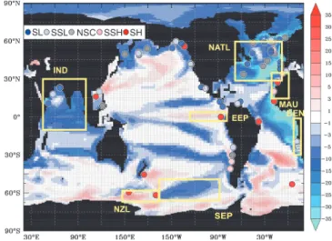
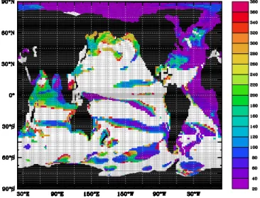
Fig. 2. FWF–GLA export differences (in gC m−2yr−1) averaged for the simulated years 350–399 (filled field), alongside paleopro-ductivity changes during Heinrich events compared to glacial mean state reconstructed from our compilation (points). Dark and light blue points represent significantly lower (SL) and slightly signifi-cantly lower (SSL) export production respectively (equivalent to “--” and ““--” or “?“--” in Table 1). Dark and light red points represent significantly higher (SH) and slightly significantly higher (SSH) ex-port production respectively (equivalent to “++” and “+” or “?+”). The grey points represent no significant change (NSC) (equivalent to “x” or “?x”).

reproduces roughly the paleoproductivity reconstruction of Kohfeld et al. (2005). One of the more consistent patterns is a dipole effect in the Southern Ocean with enhanced EXP in the middle latitudes due to increased iron deposition and decreased EXP in the high latitudes due to increased light limitation following enhanced glacial sea ice.

2.3 Experimental design

PISCES is forced offline by the atmosphere-ocean general circulation model IPSL-CM4 (Marti et al., 2010), which

in-cludes the ocean dynamical model NEMO with 2◦×2◦–0.5◦

horizontal resolution and 31 vertical levels, 10 being located in the first 100 m.

Two 400-yr-experiments have been performed under Last Glacial Maximum (LGM) conditions, with the orbital pa-rameters, greenhouse gas concentrations and ice sheets from 21 000 yr before present (see Kageyama et al., 2009 for a de-tailed presentation of the climate setup). The biogeochemi-cal simulations based on these experiments use a constant

at-mospheric CO2concentration fixed at LGM level (190 ppm)

and constant LGM dust deposition distribution (Mahowald et al., 2006), which is important for aeolian iron interac-tion with marine biology. The first experiment is an equi-librated glacial run (GLA) used as a reference run. The second experiment is a hosing experiment (FWF), starting from year 100 of the reference run. In this experiment, the

freshwater implemented in the reference run to balance snow accumulating on the ice sheets is multiplied by 2.27. This results in an additional freshwater flux of 0.1 Sv (1

Sver-drup = 106m3s−1) in the Atlantic Ocean (North of 40◦N)

and in the Arctic Ocean, which mimics the icebergs melt-ing durmelt-ing an HE. In FWF simulation, the AMOC collapses in around 250 yr. This is a relatively long time response com-pared to the simulation time but a relatively short time re-sponse compared to the resolution of most of the marine records. Indeed these records do not allow to distinguish if the changes in the AMOC happened within 10 or 400 yr. One limitation of this experimental set-up is that it uses a full LGM reference state rather than a reference state closer to the MIS3 conditions, i.e. with smaller ice-sheets, less de-pleted atmospheric greenhouse gases and orbital parameters favouring more insolation in the summer hemisphere (e.g. Van Meerbeeck et al., 2009). We chose an LGM reference state because it was closer to MIS3 conditions than a pre-industrial run and because we obtained an abrupt collapse of the AMOC for a rather small amount of freshwater hos-ing, which is relevant for the study of mechanisms occurring during Heinrich events. This is partly due to the AMOC of the reference state being rather strong and hence closer to an interstadial than to the full LGM. Besides, Heinrich events 1 and 2 did happen actually relatively close to the LGM so these conditions are also relevant for this reason.

For this study, we focus on the biogeochemical results of these simulations. Figure 1 gives an overview of the main dy-namical fields (sea surface temperature, mixed-layer depth, wind stress and Ekman pumping anomalies, sea-ice extent) useful in the interpretation of the biogeochemical results. Further ocean atmosphere dynamics details of these simu-lations can be found in Kageyama et al. (2009) where our simulations GLA and FWF correspond respectively to the simulations LGMb and LGMc.

We first study EXP as it is clearly more relevant to be com-pared with sediment core observations. But, as Taucher and Oschlies (2011) have pointed out for projection simulations, there might be cases where the response of PP and EXP to climate can be decoupled, so we will examine this potential decoupling once the fidelity of the model performance has been assessed.

In the following, we define a typical Heinrich-like event in the model through the difference between the FWF and GLA simulations averaged over the last 50 yr of the 400-yr simu-lations. We compare such a signature with our data compila-tion, where the mean response of the 7 events is considered to represent a typical HE in the observations. Nonetheless, we need to keep in mind that those reconstructions span time periods that were very different in solar irradiance due to the changes in the Earth’s orbit, which may have affected the re-sponse. The comparison between 50-yr averaged simulations and 500-yr resolution data is not ideal, but because of calcu-lation time constraints, we could only run two simucalcu-lations of 400 yr each. Schmittner (2005) and Schmittner and Galbraith

(2008) highlight the time dependence of the response in EXP to HEs. For example, full reduction in PP in the Indian and Pacific oceans is only expressed more than 1000 yr after the AMOC shutdown in their simulations. It would be interesting to consider the time component in longer simulations than what was possible in this study.

3 Results

3.1 Statistical match between model and data

In total, we found 74 marine records studies capturing at least one HE (or YD). In short, 35 record a decrease in EXP during this period, while 21 show an increase and 18 do not provide a significant trend (Table 1). If we consider the 56 records that display a significant trend, the model out-puts match 35 of these cores (Fig. 2). Among the 21 model-data mismatches, 5 of the model-data points (ODP Site 1144, Core 17950-2, GeoB3359-3, MD97-2120 and NBP9802-6PC, see Table 1 for precise location) are located on a model front area. PISCES does represent the main features of nutrients distribution, but some fronts can be shifted, due to the bi-ases of the model, so this could explain part of the mis-matches. Six of the data points (MV99 GC31/PC10, MD02-2508, MD02-2519, MD02-2524, MD02-2529 and TN057-13-4PC) are located in an area where the model does not simulate a significant change in EXP (between −1 and

1 gC m−2yr−1). Three data points (PL07-57PC,

EW0408-11JC and M23415) are displaying an increase in EXP, while other data points (respectively M35003-4 and PL07-39PC for PL07-57PC; EW0408-85JC and EW0408-66JC for EW0408-11JC; SU9039 and BOFS-5K for M23415) within the same area display a decrease in EXP just as the model does. These last data points raise the problem of compar-ing local data records to regionally averaged model cells. Even if we consider that the signal captured by marine cores has been well preserved within both the water column and the sediments, each data record is nonetheless the addition of a regional signal and a local signal. The model simu-lates only the regional part of the signal, and we would need several data points for one cell of the model to be en-tirely confident with the statistical comparison. Five points (MD04-2805 CQ, GeoB5546-2, GeoB7925-2, GeoB9526-5 and GeoB9527-5) are located on the Mauritanian coast and are clearly in contradiction with the model results. We will discuss in more details the results for this region in the fol-lowing section. Finally, the two remaining non-matching data points (GeoB3912-1 and ODP Site 1233) are both located on the coast, so there might have been continental influences on the results that are not included in our simulations.

In conclusion, if we exclude the cores located on the model front areas and the ones that do not agree regionally with other nearby records, we match the sign of the response of EXP in 73 % of the locations (35 over 48). Hence, our model

1588 V. Mariotti et al.: Marine productivity response to Heinrich events

Fig. 3. FWF–GLA silica export differences (in gSi m−2yr−1) aver-aged for the simulated years 350–399.

seems to be able to simulate the main response of EXP to HEs correctly, or at least its first order mechanisms.

3.2 Regional analysis

In order to use our model-data comparison to better un-derstand the response of EXP in key regions, we define 7 box regions (NATL, BEN, EEP, IND, MAU, NZL and SEP, acronyms defined in Table 2 and regions visible in Fig. 2). We first focus on regions where proxy data is available: either model and data are in agreement as in NATL, BEN, EEP and IND, or there is a clear contradiction as in MAU. In addition, we also specifically focus on the Southern Ocean, because of its meridionally diverse response of EXP to HEs.

3.2.1 North Atlantic

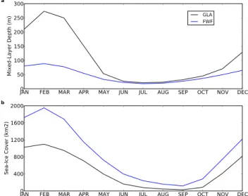
The North Atlantic (NATL) is the region where most of the marine records are located (19 in total, 13 with significant trends, see Table 1) and our modelled Heinrich-like event matches the sign of all the significant records except for one (M23415, Weinelt et al., 2003) which records a slightly significant increase in EXP while two other nearby cores (SU9039 and BOFS-5K) record a significant decrease in EXP. In the model, a shallowing winter mixed-layer depth (by more than 150 m in February, Fig. 4a) reduces the nu-trient flux to the upper ocean (not shown). This was al-ready shown in Schmittner (2005), who also gets a sim-ilar percentage decrease in EXP. Moreover, an increasing sea-ice cover (Fig. 4b) reduces light availability. Both these processes cause a decrease in EXP of 44 % (Table 2).

Gil et al. (2009) find an increase in EXP at core OCE326GGC6, located south of the present day Gulf Stream. Their data did not pass our test for significant data because the duration of their record before HE1 was less than 3000 yr, limiting the comparison to a glacial state.

Nonethe-JAN FEB MAR APR MAY JUN JUL AUG SEP OCT NOV DEC

0 400 800 1200 1600 2000

Sea-Ice Cover (km2) _piprod

b

JAN FEB MAR APR MAY JUN JUL AUG SEP OCT NOV DEC

0 50 100 150 200 250 300 Mixed-Layer Depth (m) piprodx1.15 a GLA FWF

Fig. 4. NATL area (a) mixed-layer depth (in meters) and (b)

sea-ice cover (in km2) seasonal cycle for FWF (blue) and GLA (black) simulations, averaged for the simulated years 350–399.

less, they explain this increase in EXP by an iceberg migra-tion to the subtropics inducing an isolated environment in-volving turbulent mixing, upwelled water and nutrient-rich meltwater supporting productivity. This hypothesis has not been tested in our model set-up and could not be confirmed or dismissed because (1) we do not have enough horizontal resolution to account for meso-scale processes and (2) we do not take into account nutrient input accompanying freshwater discharge.

Overall, our model matches the reduction in EXP during HEs in the North Atlantic in most cases and we suggest that the response results from greater limitation of PP and thus also of EXP by both nutrients and light.

3.2.2 Southern Ocean

In the Southern Ocean, there are 4 records indicating an increase of EXP (MD97-2120, TN057-13-14PC, E27-23, NBP9802-6PC). Our model shows significant zonal variabil-ity in this area (see Fig. 2). Nonetheless, these records are located in or close to simulated increased EXP regions. We focus here on two regions of interest that illustrate the major trends: an area in the southeast of New Zealand (NZL) and an area in the southeastern Pacific (SEP).

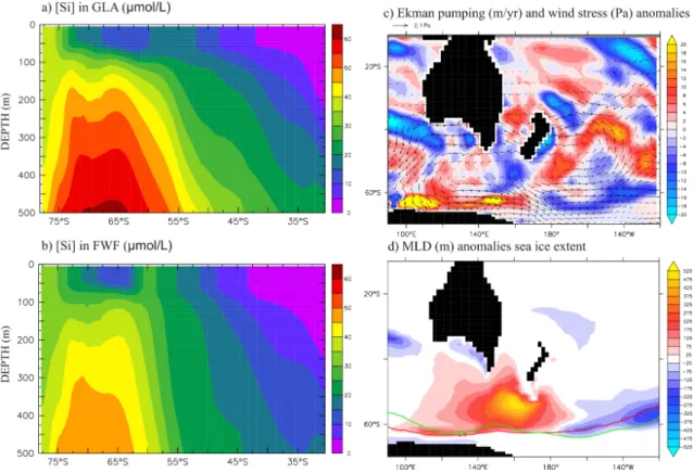
In the NZL area, south of the polar front, our model sim-ulates a 6.4 % increase in EXP (Table 2) in agreement with two different sediment cores from this same area (E27-23, NBP9802-6PC). The model suggests that a deepening of the Austral winter mixed layer (Fig. 5d), combined with a strengthening of the upwelling (see positive Ekman pumping anomalies in Fig. 5c), act together to increase the nutrient flux to the euphotic zone and stimulate PP and EXP. In par-ticular, we note an increase in silicic acid concentrations in surface waters in FWF compared to GLA (see Fig. 5a and

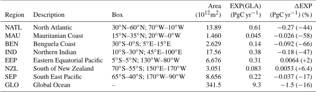
Table 2. Definition and characteristics (latitudes, longitudes, area) of the regions chosen for the data-model comparison. The column

EXP(GLA) gives the amount of carbon exported to the deep waters for each region defined. This amount is an average over the last 50 yr of simulation GLA. The column 1EXP gives the difference in carbon exported to the deep waters between the simulations FWF and GLA. For example, “−0.27 (−44)” means that in the FWF simulation, the NATL region exports 0.27 PgC yr−1less than in the GLA simulation, which corresponds to a 44 % decrease.

Area EXP(GLA) 1EXP Region Description Box (1012m2) (PgC yr−1) (PgC yr−1) (%) NATL North Atlantic 30◦N–60◦N; 70◦W–10◦W 13.89 0.61 −0.27 (−44) MAU Mauritanian Coast 15◦N–35◦N; 20◦W–0◦W 1.460 0.045 −0.026 (−58) BEN Benguela Coast 30◦S–0◦S; 5◦E–15◦E 2.629 0.14 −0.092 (−66) IND Northern Indian 10◦S–30◦N; 45◦E–100◦E 17.56 0.38 −0.18 (−47) EEP Eastern Equatorial Pacific 5◦S–5◦N; 130◦W–80◦W 6.676 0.31 0.0064 (+2) NZL South of New Zealand 70◦S–55◦S; 150◦E–170◦W 3.051 0.083 0.0053 (+6.4) SEP South East Pacific 65◦S–40◦S; 170◦W–90◦W 8.656 0.22 −0.037 (−17) GLO Global Ocean – 341.5 9.3 −1.5 (−16)

b) as suggested by Anderson et al. (2009). Silica export pos-itive anomalies in the NZL region (Fig 3) confirm this last finding. In the model, enhanced simulated wind stress inten-sifying the upwelling and retreat of Austral winter sea ice poleward (Fig. 5d) both reduce the insulation effect and in-crease the momentum flux between the atmosphere and the ocean, which induces a deepening of the mixed layer. The retreat of sea ice is itself linked to increased SST (see-saw effect, Fig. 1a).

In the SEP area, EXP decrease by 17 % in the model (Ta-ble 2), in contrast to the NZL region. Our model simulates increasing Austral winter sea ice that isolates the surface waters from the atmosphere in this area. This “barrier ef-fect” of sea ice means that winds cannot deepen the winter mixed layer enough to introduce nutrients in the upper ocean, which would be available for consumption by phytoplankton in spring. Moreover, greater sea ice also reduces the spring-time light availability. Both these processes (reduced winter mixing and less springtime irradiance) induce a decrease in EXP in this area. As far as we know, no paleo-productivity proxy with millennial-scale resolution has been published in this area, so we cannot compare our results with any recon-structions. Nonetheless, we found one sediment core (E11-2 in Mashiotta et al., 1999) displaying SST reconstructions for the last deglaciation and HE1. This core shows that SST in-creases from the LGM to the Holocene in this region, so in particular during HE1. From our model results, we would have expected a decrease of SST during HE1 in this area, to explain the simulated increased sea-ice extent. Some global climate models also find this SST anomaly in the SEP, but others do not (Kageyama et al., 2010; Merkel et al., 2010; Otto-Bliesner and Brady, 2010; Kageyama et al., 2009), thus this pattern could be model dependent. We need further high resolution data to discriminate between model results and better understand the main processes involved in this area.

Overall, our model matches the increased EXP noted in the sediment cores in the Southern Ocean, but we highlight a

large degree of spatial variability in the response of EXP to different patterns of winter mixing and sea ice.

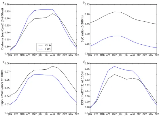
3.2.3 East Equatorial Pacific

In the East Equatorial Pacific (EEP), 5 cores studies (3 with a significant trend) are available at the same location (they appear as one red point in Fig. 2) and show an increased EXP. In this area, the model indicates a 2 % increase in EXP (Table 2), which is the result of greater equatorial upwelling due to stronger trade winds (see Fig. 1c). This mechanism increases the nutrient availability in this area and agree with concomitant decreased reconstructed SST and in-creased organic carbon content in sediment (Kienast et al., 2006). Although the model simulates an increase in EXP (Fig. 6d), it shows a simultaneous decrease in the export of silicate (Fig. 6c), a biomarker for diatoms, which might ap-pear counter-intuitive. However, laboratory data has shown that when diatoms are iron limited, they adapt to this new environment consuming more silicate relative to C and N (Hutchins and Bruland, 1998; Takeda, 1998) thereby allow-ing the export of Si and C to become decoupled; this process is included in our model. In the context of HEs, the exact op-posite happens, with diatoms experiencing greater iron avail-ability, which decreases their relative silicic acid uptake and decreases the Si/C ratio for diatoms (Fig. 6b). This process drives a decrease in the export of silicate (see also Fig. 3, EEP region), even if EXP increases. This process has already been pointed out by Pichevin et al. (2009) at ODP Site 1240 (see Table 1) for glacial/interglacial time-scales and our sim-ulations reveal that it seems to be a critical process on sub-millennial time-scales as well (see Fig. 6). The EEP is in fact a high-nutrient, low-chlorophyll (HLNC) region, which is iron-limited, so variation in the input of iron can induce high variations in EXP. As for the origin of iron, Leduc et al. (2007) showed that during HEs, the southward shift of the Intertropical Convergence Zone (ITCZ) can induce drier air

1590 V. Mariotti et al.: Marine productivity response to Heinrich events

Fig. 5. Silicic acid concentration (in µmol l−1) for (a) GLA and (b) FWF runs (transect averaged longitudinally over NZL area (see longitudes details in Table 2; (c) Ekman pumping (shaded area, in m yr−1) and wind stress (vectors, in Pa) anomalies; (d) mixed layer depth (shaded area, in m) and sea-ice extent (each contour represents the isoline of 10 % of sea-ice cover, respectively in green for the GLA run and in red for the FWF run). All the fields plotted here are averaged on months August and September for the simulated years 350–399.

that conveys more airborne iron. In our model, the airborne iron flux is kept constant at glacial levels between the two simulations, so we cannot capture this effect. Nevertheless, the model simulates greater iron supply to EEP surface wa-ters due to enhanced vertical supply. The subsurface ocean is clearly to be considered as a potential source for iron dur-ing HEs in this region. Even if the simulated increase (2 %) in EXP is fairly small, it is encouraging that our model re-produces the trend of EXP recorded in proxies, as well as capturing the decoupling between the export of carbon and silica noted in the geologic record in EEP.

3.2.4 Coastal regions

Coastal regions are not the best areas to test our model re-sults as the model cannot capture specific coastal processes because of its coarse resolution. These areas are nevertheless regions where most data are available because of an impor-tant sedimentation rate, which allows a high-resolution anal-ysis, so we endeavour to examine them. Our assumption is that the main signature found in coastal area is related to large-scale changes.

Four proxy-based studies are available on the Maurita-nian coast (MAU); they all find increased EXP in response

to HEs linked to an enhanced upwelling (Penaud et al., 2010; Holzwarth et al., 2010; Zarriess and Mackensen, 2010; Romero et al., 2008). However, in contrast to these records, our runs simulate a 58 % decrease in EXP (Table 2). We do observe an enhanced upwelling in our simulations (see pos-itive Ekman pumping anomalies in Fig. 1c) but it is com-pletely offset by the overall thinning of the mixed layer (Fig. 1b) induced by the freshwater forcing in North Atlantic. It is plausible that our idealised freshwater forcing might be too strong compared to real HEs or that the zone of fresh-water input does not exactly correspond to the region where icebergs melt.

On the Benguela coast (BEN), EXP decreases both in data (GeoB1706-2, GeoB1711-4, GeoB3606-1) and in the model (by 66 %, Table 2). In the mean glacial state, there is an im-portant upwelling in this area that decreases significantly dur-ing our HE experiment. Therefore, most of nutrient enriched sub-surface waters do not reach the euphotic layer, which re-duces EXP by increasing nutrient limitation.

In the Indian Ocean (IND), more precisely in the Arabian Sea, the model simulates decreased EXP (by 47 %, Table 2), in good agreement with high resolution data (Ivanochko et al., 2005; Higginson et al., 2004; Altabet et al., 2002; Schulte and M¨uller, 2001). In this region, EXP is primarily

V. Mariotti et al.: Marine productivity response to Heinrich events 1591

JAN FEB MAR APR MAY JUN JUL AUG SEP OCT NOV DEC 0.45 0.50 0.55 0.60 0.65 0.70 0.75 0.80 Diatoms (molC/m2 (0-200m))

piprod

a

JAN FEB MAR APR MAY JUN JUL AUG SEP OCT NOV DEC 0.50 0.55 0.60 0.65 0.70 0.75 Si/C ratio (0-200m)

b

JAN FEB MAR APR MAY JUN JUL AUG SEP OCT NOV DEC 0.02 0.03 0.04 0.05 0.06 0.07 0.08 ExpSi (molSi/m2) at 100m

c

JAN FEB MAR APR MAY JUN JUL AUG SEP OCT NOV DEC 0.27 0.28 0.29 0.30 0.31 0.32 0.33 0.34 0.35 0.36 EXP (molC/m2) at 100m

d

Fig. 6. Average on the EEP area (simulated years 350–399) of (a) diatom concentration (in molC m−2averaged on the first 200 m of the water column), (b) Si/C ratio (also averaged on the first 200 m of the water column), (c) silica export (ExpSi) at 100 m (in molSi m−2) and

(d) export production (EXP) at 100 m (in molC m−2).

controlled by upwellings, themselves induced by monsoon Westerlies (Bassinot et al., 2011). Kageyama et al. (2009) found a weaker monsoon in the Heinrich-like event simula-tion we use. This weaker monsoon thus induces weaker up-wellings and then decreased EXP.

Overall, despite the potential problems in comparing global model results to coastal sediment cores, our model succeeds in reproducing the observed trends in the BEN and IND regions. We suppose that the mismatch in the MAU re-gion could be due to the highly idealised way in which we simulate HEs.

3.3 Global analysis

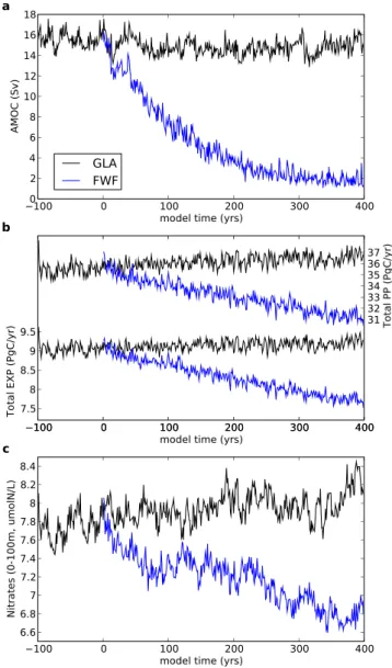
When globally integrated, EXP decreases by 16 %, or 1.5 Pg (Table 2 and Fig. 7b) by the end of the simulations, in re-sponse to a HE. EXP strongly depends on nutrients concen-trations in the illuminated waters, and the nutrient availability itself is highly dependent on nutrient supply through ocean ventilation and mixing. The constant freshwater flux that we use to approximate a HE induces a decrease of the thermoha-line circulation (shown by a reduction in the strength of the AMOC by 87 % (or 13 Sv), see Fig. 7a) associated to a strong ocean stratification in the North Atlantic. This leads to a re-duced upwelling of deep water (as already shown in Schmit-tner, 2005) and a decrease in the ventilation of the subsurface ocean, which induce a decrease of nutrient supply (cf. the

de-crease of almost 13 % of global nitrate concentration at the surface in Fig. 7c). This explains the global decrease in EXP. We note that whereas the AMOC stabilises at around 2 Sv by the end of our simulation, EXP continues to decrease linearly over the entire 400 yr period.

As explained in the experimental design section, we have chosen to compare our modeled EXP to available marine productivity data, making the hypothesis that PP and EXP are varying in the same direction. However, Taucher and Os-chlies (2011) recently showed that it is not always the case in response to climate variability. When the temperature in-creases, metabolic effects cause an increase in both PP and remineralisation of organic matter by bacteria. Greater rem-ineralisation can reduce EXP, but may also yield positive feedback on PP via the subsequent increase in available re-newed nutrients due to greater heterotrophy. In order to in-vestigate if PP and EXP respond similarly in our experiment, we plot the ratio of the comparative change in these two quantities in Fig. 8. For the areas we focused on here (Fig. 2) PP and EXP vary in the same direction, thus our modeled EXP is a correct “proxy” of PP in these areas. Alternatively, there are some regions where the model simulates opposite responses for PP and EXP. Most of these areas are located in the boundary between an increased and a decreased EXP so they may be due to horizontal advection effects. Other PP-EXP decoupled areas, like the ones south of New Zealand correspond to regions showing lower EXP, higher PP and

1592 V. Mariotti et al.: Marine productivity response to Heinrich events

100 0 100 200 300 400

model time (yrs) 0 2 4 6 8 10 12 14 16 18 AMOC (Sv)

a

GLA

FWF

model time (yrs) 6.6 6.87 7.2 7.4 7.6 7.88 8.2 8.4 Nitrates (0-100m, umolN/L)

c

Total EXP (PgC/yr)

b

100 0 100 200 300 400

model time (yrs)

31 32 33 34 35 36 37 Total PP (PgC/yr)

Fig. 7. (a) AMOC (Sverdrups, 1 Sverdrup = 106m−3s−1),

(b) globally averaged PP (primary productivity) and EXP (export

production) (PgC yr−1), (c) globally averaged nitrates concentra-tion on the first 100 m (µmol l−1) and for both simulations, GLA (black) and FWF (blue).

warmer temperatures (Fig. 8). Taucher and Oschlies (2011)’s hypothesis can thus partly explain the differences observed between PP and EXP (the parameterization of PP and rem-ineralisation is indeed dependent on temperature in PISCES).

4 Discussion

4.1 Comparison with other model studies

Other model studies have examined the response of EXP to freshwater forcing with models of intermediate complex-ity (Menviel et al., 2008; Schmittner, 2005) or atmosphere– ocean general circulation models (Obata, 2007). The

freshen-Fig. 8. Comparative change in PP (primary productivity) and EXP

(export production) (with 1X =X(FWF)−X(GLA)_X(GLA) , X averaged on simulated years 350–399) (filled field) and sea surface temperature anomaly (isolines each 0.5 degrees Celsius) for the simulated years 350–399.

ing scenarios applied were different from those employed in this study, so we cannot compare the results quantitatively, as explained by Bouttes et al. (2012) who discuss how different hosing scenarios modulate Heinrich events and their impact on the ocean carbon cycle. We can however qualitatively ex-amine the patterns in the EXP response between models.

In general, the reduced EXP in NATL and BEN are con-sistent between the models suggesting that these are robust responses to freshwater fluxes input in the North Atlantic. However, there are regions where the models have a differ-ent response to hosing. We will focus on EEP, NZL, MAU and IND. These are regions where EXP is mainly controlled by upwelling. As coarse-resolution climate models usually have difficulties to simulate upwellings correctly, we first check that upwellings are well represented in the modern version of each model before drawing any conclusion on glacial centennial-scale changes in these regions. The IPSL-CM4 model represents all these upwellings (Bassinot et al., 2011; Steinacher et al., 2010; Lenton et al., 2009; Schnei-der et al., 2008) though it tends to unSchnei-derestimate their inten-sity both in terms of upwelled water flux and surface pro-ductivity. The LOVECLIM model represents the EEP and NZL upwellings but not the MAU and IND ones (see Men-viel et al., 2008, Figs. 5 and 6). The UVic model represents the EEP, NZL and IND upwellings, but not the MAU one (see Schmittner, 2005, Fig. 2). The MRI model represents all the upwellings (see Obata and Kitamura, 2003, Fig. 3a). We need also to point out that while Menviel et al. (2008)’s, Obata (2007)’s and our simulations are performed with inter-active winds, Schmittner (2005)’s simulations use prescribed modern winds, so his simulations cannot capture wind-driven changes in upwellings.

In EEP and most of the Southern Ocean, we find an in-creased EXP which is in contrast to the three previous model studies. Note however that when forced by changes in

inso-lation and CO2for HE1, LOVECLIM also simulates an

in-crease in EXP for the Southern Ocean (Menviel et al., 2011). For both regions, we attribute this difference to the wind-driven increased upwelling. We explain the difference with Schmittner (2005)’s study by his non representation of winds changes. For Menviel et al. (2008)’s and Obata (2007)’s stud-ies that do represent these upwelling areas in modern times and computes wind changes, we need to find other explana-tions. We hypothesise that the discrepancies between Men-viel et al. (2008)’s model and ours are probably due to two factors. On one hand, our model has an increased atmo-spheric resolution, so we hypothesise it captures better the wind changes in upwelling areas. On the other hand, our model has a parameterization of Si/C as a function of temper-ature and iron availability that is not implemented in LOVE-CLIM and we have shown in the results section that this pa-rameterization was key to simulate the EEP region changes. For the discrepancies between Obata (2007)’s model and ours, the explanation is different. The MRI-CGCM2 model has a comparable resolution to the IPSL-CM4 one, so the discrepancies cannot come from a problem of low resolution winds representation. In Obata (2007)’s Heinrich-like sim-ulation, the sea-ice cover increases in the Southern Ocean, which should induce a shallower mixed layer and also a de-creased upwelling. This can explain why the MRI-CGCM2 model simulates a decreased EXP in this area. For the EEP region, the MRI-CGCM2 model does not have either the pa-rameterization of Si/C implemented in the PISCES model, so the model is not able to simulate an increase in EXP. Nonetheless, the EEP region is fairly narrow in our simu-lations and is bounded to the north and south by negative EXP anomalies, so we would need further marine records to document this area and draw robust conclusions.

In IND, our study finds a decrease in EXP due to a weaker upwelling as do Schmittner (2005) and Obata (2007), whereas Menviel et al. (2008) simulate an increase in EXP. As Schmittner (2005)’s simulations use prescribed preindus-trial winds, the decrease in upwelling seen in his simulations is thermohaline-driven. As explained above, the modern sim-ulations of LOVECLIM do not represent the upwelling in this area, so it cannot obviously simulate changes of up-welling regimes.

In MAU, the decreased EXP we simulate is at odds with both data and previous model studies, which present an in-creased EXP due to an enhanced upwelling. We need to ex-plain why our model, supposed to be able to capture changes in wind-driven upwellings, is not able to capture the signal of increased productivity seen in data. We make the hypoth-esis that it is due to the location of our hosing. The

hos-ing is applied between 40◦N and 90◦N in our experiment,

which is south enough to make the freshwater being ad-vected through the subtropical gyre directly to the

Maurita-nian coast. On the contrary, in the other studies, the hosing is

applied more northward (between 50◦_{N and 65}◦_{N for}

Men-viel et al. (2008), between 50◦_{N and 70}◦_{N for Obata (2007)}

and between 45◦N and 65◦N for Schmittner (2005)), which

makes the freshwater flow northward through the North At-lantic Current. Hence, the surface waters are considerably mixed through the subpolar gyre before they arrive on the Mauritanian coast. We do have an increase of upward ver-tical velocities in the upper ocean of this region (see pos-itive Ekman pumping in the Mauritanian coast in Fig. 1c), but this increased upwelling is completely balanced by the freswater lid that does not allow the nutrients to spread out from the subsurface waters. In addition, the modern simula-tions previously performed with our model (Steinacher et al., 2010) display a really weak upwelling in this area compared to data, so this underestimation of vertical velocities can ex-plain why it cannot balance the lid effect. Nonetheless, the other studies simulate an increase in productivity in MAU. This is understandable for Obata (2007) because the MRI-CGCM2 model represents the Mauritanian upwelling and the simulations have interactive winds. As seen before, the two other studies do not represent properly the Mauritanian up-welling in preindustrial settings. The greater EXP obtained in Menviel et al. (2008) off the Mauritanian coast might be due to a greater upwelling and/or an increase in nutrient con-tent in the source water. Indeed, the stratification generated in the North Atlantic by the freshwater input leads to a sub-surface positive nutrient anomaly, which is advected to lower latitudes. In Schmittner (2005), as the surface winds are con-stant, the EXP increase in MAU is mainly due to a greater thermohaline driven upwelling and/or a greater nutrient con-tent in the source water. To summarise, in MAU, according to data, there was an enhanced upwelling during HEs inducing increased EXP, but our model cannot reproduce it because of (1) a too weak intensity of the upwelling in modern times and (2) a freshwater forcing too close to the upwelling area.

In conclusion, the differences between model results come mostly from atmospheric resolution and biogeochemical pa-rameterization differences but also from the different loca-tions of freshwater forcing and the way the models advect them from the area of freshening. Overall, except for the Mauritanian coast, our study correctly simulates the response of EXP to HEs, and points out the importance of the Si/C ratio parameterization in marine biogeochemical models. 4.2 What do these results tell us for 21st century

projections?

We do not yet have any certainty on the sign of the global evolution of marine PP with global warming (Taucher and Oschlies, 2011). Investigating the response of marine bio-geochemical models to HEs could be of use in examin-ing the predicted impact of climate change on marine bio-geochemistry. Valdes (2011) recently pointed out that the coupled climate models might be too stable to simulate

1594 V. Mariotti et al.: Marine productivity response to Heinrich events abrupt centennial-scale changes like the actual global

warm-ing and that they need to be tested on past abrupt climate changes. This study shows that the model IPSL-CM4 includ-ing PISCES is able to represent the main features of EXP response to a HE, except for the Mauritanian region which needs to be further investigated. With the sediment data cur-rently available, we are not able to test if the model an-swers quantitatively well. We need further more attempts of PP or EXP calibration from different biomarkers as it has been done by Salgueiro et al. (2010), Voelker et al. (2009) or Beaufort et al. (1997) to have a more direct comparison with our model outputs. Nonetheless, the model can simulate an EXP response to HEs qualitatively consistent with avail-able data, and more importantly with a fast time response in certain regions, like in the Atlantic Ocean which responds strongly within a hundred years (see Fig. 9). Even with an AMOC decreasing on slower timescales (' 250 yr), PISCES model forced by IPSL-CM4 output seems to be able to sim-ulate transient climate changes on centennial scales. This is encouraging as it has been used for climate projections. The problem with the Mauritanian upwelling system needs though to be fixed in the future for more reliable projections, as this upwelling system is very important for future food (e.g. fish) supply. Finally, we need to point out that while our model simulates a global decrease of PP by 16 % with HEs, we still do not have any global constraint to validate this re-sult. New isotopic methods using for instance the triple iso-topes (Landais et al., 2007) or the Dole effect (Landais et al., 2010) should be used to investigate this result. Simulating HEs could be a benchmark for coupled climate carbon cy-cle models to test their ability to simulate abrupt transient climate changes, and our compilation of paleoproductivity proxies could be compared to the results of the models.

Studying the response of EXP to HEs can also give in-sights of mechanisms that may affect EXP under global

warming. The radiative effect of increased CO2and

subse-quent warming on marine biology has already been tested. Steinacher et al. (2010) performed a model inter-comparison between four coupled climate-carbon cycle models for future climate. Significant regional differences between the mod-els in the response of EXP to climate change appear but there are shared patterns like a decrease of EXP in NATL and an increase in the Southern Ocean. Global warming is also accompanied by a melting of the Greenland ice sheet, which is not taken into account in most of the actual cou-pled models. Our study could represent an analogue to this future Greenland melting, which is implemented in the study of Steinacher et al. (2010) only for one model (IPSL-CM4) out of four models. Of course our study starts with a glacial climate background so this could induce differences in the intensity of the response of the system compared to the same freshwater forcing with an interglacial climate background, so we need to be careful when comparing our HEs simu-lations with global warming freshwater forcing projections. Nonetheless, we can point out some significant trends, like a

Fig. 9. FWF–GLA time response (in years) of EXP (export

produc-tion): defined as the time after which half of the final signal (aver-aged on the simulated years 350–399) in EXP has been reached. We only considered regions where the final anomaly of EXP was more than 1 gC m−2yr−1in absolute value: the white areas in the ocean do not have such an important anomaly in the end.

decrease of EXP in the North Atlantic, a region that is already projected to undergo a decrease of EXP due to global warm-ing. This result is in agreement with the fact that the IPSL model in Steinacher et al. (2010) study was already simulat-ing a more important decrease in this region. Hence, actual projections may underestimate the decrease of EXP in this region. Swartz et al. (2010) have shown that actual increased fishing induces a higher percentage of required PP to sustain global fish populations, with a special increase in North At-lantic Ocean. Projections including a freshwater forcing may be of use to help constraining EXP response in the future, especially for the areas of actual intense fishing that could be strongly affected in the coming decades.

5 Conclusions

This study first aimed at evaluating the response of a marine biogeochemistry model (PISCES) to centennial-scale events in glacial times, using marine cores for comparison. Despite the fact that we used full glacial boundary conditions rather than more realistic MIS3 conditions, the model results re-garding the response of marine biology to Heinrich events are most of the time qualitatively consistent with paleo-data, which is encouraging for its ability to simulate future cli-mate impacts on primary productivity and especially abrupt centennial-scale changes. The data compilation for paleopro-ductivity we gathered and used to test our model results can be used as a tool to evaluate other coupled biogeochemical-climate model responses to Heinrich events and their abil-ity to simulate a centennial-scale climate change. Our work

also highlights the importance of the Si/C ratio parameteri-zation in models as a key mechanism to simulate certain re-gions ecosystem, here in the Eastern Equatorial Pacific. This study also points out the importance of multi-proxy analysis to interpret paleoproductivity in the sediments.

The second aim of this study was to use the model to more accurately understand the global and regional response of marine productivity to Heinrich events. We simulate a global decrease of primary productivity of 16 % following the fresh-water forcing, with some regional differences. According to our data-model intercomparison, it is very likely that the North Atlantic Ocean, the southwestern coast of Africa and the Indian Ocean experienced a decrease in primary produc-tivity, whereas the Southern Ocean and the Eastern Equato-rial Pacific experienced an increase during Heinrich events. This study also gives us an insight of what could be the con-tribution of a melting of Greenland ice sheet in the coming century: an accentuated decrease of organic matter export in the North Atlantic Ocean.

Supplementary material related to this article is available online at: http://www.clim-past.net/8/1581/ 2012/cp-8-1581-2012-supplement.pdf.

Acknowledgements. We thank the French National Computing

Center CEA/CCRT for the computer time provided. This is Past4Future contribution no. 34. The research leading to these results has received funding from the European Union’s Seventh Framework programme (FP7/2007-2013) under grant agreement no. 243908, “Past4Future. Climate change – Learning from the past climate”.

Edited by: T. Kiefer

References

Altabet, M., Higginson, M., and Murray, D.: The effect of millennial-scale changes in Arabian Sea denitrification on atmo-spheric CO2, Nature, 415, 159–162, doi:10.1038/415159a, 2002.

Anderson, R., Ali, S., Bradtmiller, L., Nielsen, S., Fleisher, M., An-derson, B., and Burckle, L.: Wind-driven upwelling in the South-ern Ocean and the deglacial rise in atmospheric CO2, Science,

323, 1443–1448, doi:10.1126/science.1167441, 2009.

Arellano-Torres, E., Pichevin, L., and Ganeshram, R.: High-resolution opal records from the eastern tropical Pacific pro-vide epro-vidence for silicic acid leakage from HNLC regions during glacial periods, Quaternary Sci. Rev., 30, 1112–1121, doi:10.1016/j.quascirev.2011.02.002, 2011.

Aumont, O. and Bopp, L.: Globalizing results from ocean in situ iron fertilization studies, Global Biogeochem. Cy., 20, GB2017, doi:10.1029/2005GB002591, 2006.

Bard, E., Rostek, F., Turon, J., and Gendreau, S.: Hydrological impact of Heinrich events in the subtropical northeast Atlantic, Science, 289, 1321–1324, doi:10.1126/science.289.5483.1321, 2000.

Barron, J. A., Bukry, D., Dean, W. E., Addison, J. A., and Finney, B.: Paleoceanography of the Gulf of Alaska dur-ing the past 15,000 years: Results from diatoms, silicoflagel-lates, and geochemistry, Mar. Micropaleontol., 72, 176–195, doi:10.1016/j.marmicro.2009.04.006, 2009.

Bassinot, F., Marzin, C., Braconnot, P., Marti, O., Mathien-Blard, E., Lombard, F., and Bopp, L.: Holocene evolution of summer winds and marine productivity in the tropical Indian Ocean in re-sponse to insolation forcing: data-model comparison, Clim. Past, 7, 485–520, doi:10.5194/cp-7-815-2011, 2011.

Beaufort, L., Lancelot, Y., Camberlin, P., Cayre, O., Vincent, E., Bassinot, F., and Labeyrie, L.: Insolation cycles as a major con-trol of equatorial Indian Ocean primary production, Science, 278, 1451–1454, doi:10.1126/science.278.5342.1451, 1997. Bopp, L., Monfray, P., Aumont, O., Dufresne, J., Le Treut, H.,

Madec, G., Terray, L., and Orr, J.: Potential impact of climate change on marine export production, Global Biogeochem. Cy., 15, 81–99, doi:10.1034/j.1600-0889.2003.042.x, 2001.

Bopp, L., Kohfeld, K., Le Quere, C., and Aumont, O.: Dust impact on marine biota and atmospheric CO2during glacial periods,

Pa-leoceanography, 18, 1046, doi:10.1029/2002PA000810, 2003. Bouttes, N., Paillard, D., and Roche, D.: Impact of brine-induced

stratification on the glacial carbon cycle, Clim. Past, 6, 681–710, doi:10.5194/cp-6-575-2010, 2010.

Bouttes, N., Roche, D. M., and Paillard, D.: Systematic study of the impact of fresh water fluxes on the glacial carbon cycle, Clim. Past, 8, 589–607, doi:10.5194/cp-8-589-2012, 2012.

Bozbiyik, A., Steinacher, M., Joos, F., Stocker, T. F., and Menviel, L.: Fingerprints of changes in the terrestrial carbon cycle in re-sponse to large reorganizations in ocean circulation, Clim. Past, 7, 319–338, doi:10.5194/cp-7-319-2011, 2011.

Broecker, W., Bond, G., Klas, M., Clark, E., and McManus, J.: Ori-gin of the northern Atlantic’s Heinrich events, Clim. Dynam., 6, 265–273, doi:10.1007/BF00193540, 1992.

Brunelle, B. G., Sigman, D. M., Jaccard, S. L., Keigwin, L. D., Plessen, B., Schettler, G., Cook, M. S., and Haug, G. H.: Glacial/interglacial changes in nutrient supply and stratifica-tion in the western subarctic North Pacific since the penulti-mate glacial maximum, Quaternary Sci. Rev., 29, 2579–2590, doi:10.1016/j.quascirev.2010.03.010, 2010.

Cacho, I., Grimalt, J., Pelejero, C., Canals, M., Sierro, F., Abel Flo-res, J., and Shackleton, N.: Dansgaard-Oeschger and Heinrich event imprints in Alboran Sea paleotemperatures, Paleoceanog-raphy, 14, 698–705, doi:10.1029/1999PA900044, 1999. Calvo, E., Pelejero, C., Pena, L., Cacho, I., and Logan, G.: Eastern

Equatorial Pacific productivity and related-CO2 changes since

the last glacial period, Proc. Natl. Acad. Sci., 108, 5537–5541, doi:10.1073/pnas.1009761108, 2011.

Cartapanis, O., Tachikawa, K., and Bard, E.: Northeastern Pacific oxygen minimum zone variability over the past 70 kyr: Impact of biological production and oceanic ventilation, Paleoceanogra-phy, 26, PA4208, doi:10.1029/2011PA002126, 2011.

Dannenmann, S., Linsley, B., Oppo, D., Rosenthal, Y., and Beau-fort, L.: East Asian monsoon forcing of suborbital variability in the Sulu Sea during Marine Isotope Stage 3: Link to North-ern Hemisphere climate, Geochem. Geophy. Geosy., 4, 1001, doi:10.1029/2002GC000390, 2003.

Dean, W. E.: Sediment geochemical records of productivity and oxygen depletion along the margin of western North America