HAL Id: halshs-00965549
https://halshs.archives-ouvertes.fr/halshs-00965549v2
Preprint submitted on 19 May 2014
HAL is a multi-disciplinary open access archive for the deposit and dissemination of sci-entific research documents, whether they are pub-lished or not. The documents may come from teaching and research institutions in France or abroad, or from public or private research centers.
L’archive ouverte pluridisciplinaire HAL, est destinée au dépôt et à la diffusion de documents scientifiques de niveau recherche, publiés ou non, émanant des établissements d’enseignement et de recherche français ou étrangers, des laboratoires publics ou privés.
Is Self-Reported Risk Aversion Time Varying?
Seeun Jung, Carole Treibich
To cite this version:
Seeun Jung, Carole Treibich. Is Self-Reported Risk Aversion Time Varying?. 2014. �halshs-00965549v2�
WORKING PAPER N° 2014
– 12
Is Self-Reported Risk Aversion Time Variant?
Seeun Jung Carole Treibich
JEL Codes: C33 ; D31 ; J11 Keywords: Risk Aversion; Panel Data
P
ARIS-
JOURDANS
CIENCESE
CONOMIQUES48, BD JOURDAN – E.N.S. – 75014 PARIS
TÉL. : 33(0) 1 43 13 63 00 – FAX : 33 (0) 1 43 13 63 10
www.pse.ens.fr
Is Self-Reported Risk Aversion Time
Variant?
Seeun Jung
∗and Carole Treibich
†Abstract
We examine a Japanese Panel Survey in order to check whether self-reported risk aversion varies over time. In most panels, risk attitude variables are collected only once (found in only one survey wave), and it is assumed that self-reported risk aversion reflects the individual’s time-invariant component of preferences to-ward risk. Nonetheless, the question could be asked as to whether the financial and macro shocks a person faces over his lifetime modify his risk aversion. Our em-pirical analysis provides evidence that risk aversion is composed of a time-variant part and shows that the variation cannot be ascribed to measurement error or noise given that it is related to income shocks. Taking into account the fact that there are time-variant factors in risk aversion, we investigate how often it is preferable to collect the risk aversion measure in long panel surveys. Our result suggests that the best predictor of current behavior is the average of risk aversion, where risk aversion is collected every two years. It is therefore advisable for risk aversion measures to be collected every two years in long panel surveys.
JEL Classification: C33 ; D31 ; J11 Keywords: Risk Aversion; Panel Data
∗Paris School of Economics, Science-Po Paris - [email protected]
†Paris School of Economics, Erasmus University Rotterdam and Aix-Marseille University
1
Introduction
Is risk aversion innate and immutable, as is usually assumed in the economic literature, or rather time-variant and a function of a persons experiences over his lifetime? Basically, do individual preferences toward risk change with such events as wealth accumulation, disease, job loss and parenthood? Given that the psychology literature suggests that personality can change over time (Lucas and Donnellan (2011), Boyce et al.(2013)), we ask the question as to whether individual risk attitudes can also vary across the life span. Risk preferences have been extensively used in empirical work to study individual decision-making. It is therefore vital to gain a better understanding of what surveys actually capture and whether this variable might vary across fields or over time. In other words, what researchers need to address when using risk attitudes taken from micro-level data surveys is the validity of the drawn risk aversion parameter. Although a great deal of empirical literature on this issue focuses on the measurement of risk tolerance and its stability across methodologies,1
the question of the stability of risk aversion over time is assumed rather than proven empirically.2
Nevertheless, the sensitivity of risk aversion to financial and personal shocks can be problematic since it could cause endogeneity or reverse causality issues when preferences toward risk are used as an explanatory variable. For example, imagine someone wins a lottery (positive income shock), which possibly drives down his risk aversion. If we only have one risk aversion measure, which was collected when he was more risk averse, the coefficient estimated taking this measure in order to predict current behavior would be biased toward zero (underestimation). So investigating whether risk attitudes are stable or changeable, and if they are changeable, finding these variations main factors are crucial steps if we are to make proper use of survey data.
1
See for instanceBinswanger(1980),Anderson and Mellor(2008),Ding et al.(2010),Dohmen et al. (2011) andHardeweg et al.(2012)
2
WhileHarrison et al.(2005),Baucells and Villass (2010),Sahm(2008), and Andersen et al.(2008) claim that risk aversion is stable over time,Staw(1976),Thaler and Johnson(1990),Weber and Zuchel (2005), Brunnermeier and Nagel (2008), and Malmendier and Nagel (2011) find a change in financial risk-taking behaviors over time.
The main problem researchers face when investigating the time stability of individual risk tolerance is data availability. In economic theory, risk aversion is assumed to be innate and time invariant, i.e. it is considered to be an exogenous characteristic of the person. This has led many surveys to include risk attitude questions only once: namely, at baseline, when the individual enters the database. This is, for instance, the case with the British Household Panel Study (BHPS) and the Korean Labor Income Panel Study (KLIPS). Nonetheless, some surveys do repeatedly measure risk attitudes. For example, the Health and Retirement Study (HRS) includes hypothetical gambles with respect to lifetime income in all its waves. Sahm (2008) uses this feature of the data to investigate the stability of individual risk tolerance.
In this article, we use the Osaka Panel Study where individuals were surveyed annually from 2003 to 2010 and risk aversion questions were included in all waves. This framework enables us to explore whether the risk aversion responses of individuals who experience shocks are stable. Basically, we set out to provide evidence of the existence of a time-variant component of risk aversion and to shed light on the factors that influence this aspect of risk preferences. Using panel data and a self-reported risk aversion measure, we find empirical evidence that (i) survey risk aversion has a time-variant dimension, and that (ii) individuals for whom elicited risk attitudes vary experience specific shocks not faced by agents with stable risk preferences. We believe that the expected, significant correlation between the observed variation in individual risk aversion and shocks (in terms of income, labor and personal belongings) provides convincing evidence of the existence of a time-variant component of risk aversion, possible measurement error (noise) aside. Basically, our results roughly show that (self-reported) risk aversion changes every year and is affected by income and health variations. This finding suggests that variation over time is more than merely noise, since it is correlated with recent shocks. Nevertheless, the variation in risk attitudes does not appear to significantly affect the change in risky behavior, i.e. the time-variant component of risk preferences might be temporary and
not large enough to change a persons behavior.
When collecting panel data, the assumption of risk aversion stability is used in sup-port of the choice of measuring preferences toward risk only once (often during the first wave). However, given that there are time-varying factors in risk aversion, collecting risk aversion more than once could improve the quality of the analyses. Our findings show that using an average measure of risk aversion increases predictive power for current be-haviors compared to the use of current risk aversion. It provides a guideline for longer panels: it could be useful to collect risk aversion several times, since the age factor and accumulation of changes in income and health also determine risk attitudes.
The remainder of the paper is organized as follows. The related literature is presented in section 2. Section 3 discusses the potential time-variant and time-invariant factors of risk aversion and presents the data used in this paper. The existence of a time-variant component is highlighted in section 4 along with the respective importance of the two dimensions of risk aversion. This section also provides evidence of optimal times for collecting risk aversion in panel surveys. Section 5 concludes.
2
Literature
Risk preference is a key factor put forward by economists to explain individual decisions. Many published articles have emphasized the influence of risk aversion on risky behaviors in financial matters (portfolio assets, savings and indebtedness), in the choice of occupa-tion (sector of work and risky tasks) and in health (smoking and drinking). At the same time, the most suitable way of measuring risk aversion, which is not a directly observable individual characteristic, has been extensively investigated. A range of different method-ologies have been used from qualitative scales and hypothetical questions to summated rating scores and lotteries. In addition to this methodological literature, many studies look at the stability of risk aversion across methodologies in order to see whether some
measures outperform others in their capacity to predict risky behaviors. Yet the stability of individual preferences toward risk over time has not really been investigated empiri-cally. This could be due to: (i) the theoretical assumption that risk aversion is innate and immutable, and (ii) the lack of data available to study this issue.
In the theoretical models put forward by Constantinides (1990) and Campbell and Cochrane(1999), risk aversion varies with changes in wealth, habits and background risk. In a more recent consumption-based pricing model, Brandt and Wang (2003) included a time-varying aggregate risk aversion parameter and empirically tested whether aggregate risk preferences do indeed vary in response to news about inflation using DRI consumption data.
The empirical studies focusing on time-varying risk aversion consider different mea-sures of risk aversion. Brunnermeier and Nagel (2008), for instance, used asset allocation to proxy risk preferences and found that transitory increases in liquid wealth play no role in explaining changes in asset allocation for households that participate in the stock market. Guiso et al. (2013) drew on a repeated survey of a large sample of Italian Bank customers to measure individual risk attitudes using a Holt and Laury (2002) strategy. Basically, respondents were asked to choose between a fixed lottery and different safe amounts.3,4
They investigated its stability based on the 2008 financial crisis. These au-thors found that changes in risk aversion after the crisis were correlated with portfolio choices, but not with wealth, consumption habits or background risk. The authors subse-quently conducted a lab experiment where participants were exposed to a horror movie. This experiment showed that this particular psychological factor - fear - could influence risk aversion to a greater extent than its ‘classical standard’ determinants. Sahm (2008) studied hypothetical gambles with lifetime income from the 1992-2002 Health and
Re-3
In the risky outlook, individuals had a fifty percent chance of earning 10,000 euros and a fifty percent chance of earning nothing. The sure amounts of money offered ranged between 100 and 9,000 euros.
4
Where Holt and Laury (2002) offered two lotteries with different pay-off spreads, Hardeweg et al. (2012) andDohmen et al.(2010) also used a fixed lottery vs. safe amounts to capture the risk aversion of rural Thai farmers and German citizens respectively.
tirement Study to investigate whether individuals changed their risk aversion over that period. She found that risk tolerance changes with age and macroeconomic conditions, but argued that differences in risk aversion are mainly located across, and not within, in-dividuals. She took a panel of 12,000 respondents covering a decade and found relatively stable risk preferences. She showed that major life events such as job displacement and the diagnosis of a serious health condition do not permanently alter the willingness to take further risks.
However, other studies have argued that individual risk tolerance can change follow-ing health shocks. De Martino et al. (2010) found that amygdala-damaged patients5
take risky gambles more often than those without brain damage. Tison et al. (2012) also in-vestigated the influence of health shocks on an individual’s preferences toward risk. They found that some diseases do change people’s risk preferences. Basically, they showed that cancer (as a threat to an individual’s life and reduced life expectancy) increases risk tol-erance while diabetes (a long-term disease with daily treatment) increases risk aversion. A question raised subsequently by the authors is whether the observed change in risk aversion endures in the future or whether it is merely a temporary alteration of risk at-titudes, in which case risk aversion would eventually return to the individuals initial level.
In this paper, we use the information on risk aversion provided by the Osaka Panel Study. Like Sahm (2008), we investigate the existence and importance of a time-variant component of risk aversion. We show that variations in individual risk aversion are related to income and personal shocks. Sahm (2008) pointed out that a large proportion of risk aversion differences comes from differences across individuals, which implies that the time-variant component of risk preferences only plays a small role. We further investigate this dimension by studying whether variation in risk aversion is reflected by a change in individual risky behaviors. We find that risk aversion indeed contains both time-invariant and time-variant factors. Time-variant factors are correlated with various changes such
5
as income and age, which provides evidence that variations in risk aversion over time are not just noise. That is why risk aversion measures collected back in time (more than five years previously in our sample) do not predict current behavior well enough to see its effect. We will discuss this in Section 4.
3
Methodology and Data
Time-invariant and time-variant components of risk aversion
Table 1 presents the factors involved in the different explanations of risk aversion. Ba-sically, we decompose risk aversion into a time-invariant and a time-variant component. Whereas the former may be determined by family background and early childhood ed-ucation, the latter could be the result of shocks and experiences faced by individuals over their lives. Ethnicity and gender are dictated by birth. It has been widely proven that gender partially explains the difference in risk aversion (Croson and Gneezy (2009) and Bertrand (2011)). There are two aspects that may explain why women are more risk averse than men: (i) women are innately/inherently more risk averse than men at birth, (ii) their socialization in the society in which they live makes them become more risk averse. Furthermore, pre-adulthood, risk aversion may be influenced by family back-ground, early childhood education and social norms. In other words, risk aversion can be affected when individuals are building their identities and personalities. For example, individuals raised in a conservative society tend to declare a higher level of risk aversion. The samples used to measure risk aversion from surveys are generally made up of adults. So in this case, the two factors that are innate characteristics and childhood socialization can be treated as time-invariant factors. However, time-variant factors include socio-demographic characteristics and shocks that can vary over time. Risk aversion varies with age: the older an individual, the more risk averse (Tymula et al. (2013)). More-over, when an unexpected negative event, such as a health shock (accident or disease) or an income shock (job loss), happens to someone, this person might be expected to
become more risk averse due to the experience of a negative situation affecting his initial wealth (Kihlstrom et al. (1981)). In our paper, we discuss the formation of the risk aver-sion function considering both time-variant and time-invariant factors. We then look at which factor explains most of the risk-related behaviors.
Table 1: Factors Influencing the Different Dimensions of Risk Aversion
Time-invariant Time-variant
innate/physical social/early childhood
ethnicity family background socio-demographic characteristics
gender initial education - age/vocational training
- health status
- occupational characteristics
(seniority in a sector, job security level, type of wage) shocks
- income/debt/loan/inheritance - marriage/child birth/relative’s death - labor/sector/occupation/unemployment - social group, community, peer intervention - health
Data
Our investigation into the instability of risk aversion uses data collected by the University of Osaka, Ritsumeikan University, and Waseda University in Japan. This survey was launched6
in order to study the influence of economic behavior on preferences and degrees of life satisfaction. A representative sample was chosen by means of random sampling. Detailed information was collected every year from 2003 to 2010 (eight waves).7
6
This survey was launched by Yoshiro Tsutsui, University of Osaka.
7
All municipalities were classed into ten areas (1.Hokkaido, 2.Touhoku, 3.Kantou, 4.Koushinetsu, 5.Hokuriku, 6.Toukai, 7.Kinki, 8.Chugoku, 9.Shikoku, and 10.Kyushu). In each area, the municipalities were then divided into four categories corresponding to their population sizes (1.Seirei shitei toshi: A city designated by government ordinance, 2. A city with 100 thousand people or more, 3. A city with less than 100 thousand people, 4.A town or village). This gave a total of 40 strata. The number of observations in an area was determined based on a 20-to-69-year-old population and city size.
- Sampling Spot Selection (First Sampling Unit)
1) The sampling unit for the first stage (FSU) was the census unit set up by the last census. 2) Sampling spots were distributed based on population (approximately 15 samples per spot).
The same individuals were interviewed face-to-face over this period, which means we can control for unobserved heterogeneity using a panel dataset. In addition to extensive socio-demographic data (age, gender, religion, marital status and education) and eco-nomic information (occupational characteristics, income and consumption expenditure), respondents were asked to provide data on risky choices in finance (assets, loans and gambles) and health (exercise, smoking, drinking, height and weight). The survey also included gambling or lottery questions to collect data on individual risk preferences. Un-fortunately, the precise formulation of these gambling or lottery questions changed from one survey wave to the next. Yet the formulation of the few self-reported risk aversion questions remained the same from one year to another, such that we were able to use them in our panel analysis.
Table2presents a simple descriptive statistics summary of respondents’ characteristics for each wave. On average, we observe more women (over 50%) in the sample, and the average age is around 50 years old. The panel is unbalanced as some individuals were lost over the years and new participants were recruited in 2004, 2006 and 2009. Basically, the oldest respondents drop out from the sample.8
The people in the sample have 1.3 children on average, and more than half of them are gainfully employed. More than half of the Japanese people take part in some type of gambling9
. More than half of the of FSUs in the stratum). FSUs were determined by systematic sampling.
4) Each municipality in each stratum was ordered with a municipality code determined by government. -Selection of Individuals
Some 15 observations were randomly sampled by systematic sampling in each spot (FSU). The sampling interval varied by inhabitant list arrangement type.
-Selection of New Sampling Spots
Sampling spots, covering 4,600 new samples in the second survey (2003), were taken on a continuous basis from the previous survey (first survey in 2002), and the remaining spots needed were selected by the above method (First Sampling Unit)
-Use of Residential Map for Sampling in a Field
Quota sampling based on sex and age in each sampling spot was applied to the selection of 6,000 new samples in the 2009 wave since the official inhabitant list was not available. The sampling spots were taken on a continuous basis from the previous survey, and households were selected by systematic sampling using a residential map.
8
This explains why the average age does not increase between 2003 and 2004. In addition, more male participants quit over the years through to 2008. In 2009, more men and more educated/employed participants were newly recruited into the sample.
9
The British Gambling Prevalence Survey found that 73% of the British adult population (aged 16 and over) participated in some form of gambling in 2009. This is equivalent to around 35.5 million adults.
Table 2: Descriptive Statistics: Yearly
2003 2004 2005 2006 2007 2008 2009 2010
Female 0.511 0.527 0.531 0.529 0.534 0.541 0.530 0.532
(0.500) (0.499) (0.499) (0.499) (0.499) (0.498) (0.499) (0.499)
Age (in years) 49.14 49.07 50.07 50.23 51.44 52.70 49.96 51.23
(12.74) (12.97) (12.97) (13.11) (12.85) (12.66) (13.31) (13.15)
Education (in years) 12.60 12.67 12.67 12.73 12.77 12.78 13.02 13.07
(2.12) (2.14) (2.27) (2.29) (2.25) (2.25) (2.22) (2.20)
Income (in mil Yen) 3.49 3.56 3.69 3.73 3.79 3.81 3.73 3.84
(0.34) (0.35) (0.35) (0.34) (0.34) (0.33) (0.33) (0.32) Married 0.760 0.774 0.791 0.786 0.795 0.805 0.786 0.798 (0.428) (0.419) (0.407) (0.410) (0.404) (0.396) (0.410) (0.402) Children 1.252 1.294 1.326 1.324 1.375 1.411 1.386 1.436 (1.135) (1.094) (1.119) (1.146) (1.139) (1.119) (1.127) (1.144) Working 0.561 0.576 0.573 0.583 0.582 0.575 0.673 0.647 (0.496) (0.494) (0.495) (0.493) (0.493) (0.494) (0.469) (0.478) Gamble 0.571 0.605 0.624 0.586 0.606 0.592 0.605 0.703 (0.495) (0.489) (0.484) (0.493) (0.489) (0.491) (0.489) (0.457) Smoke 0.345 0.316 0.306 0.288 0.276 0.254 0.260 0.244 (0.484) (0.476) (0.473) (0.463) (0.500) (0.500) (0.500) (0.500) Drink 0.572 0.561 0.566 0.556 0.564 0.558 0.554 0.531 (0.408) (0.416) (0.415) (0.410) (0.402) (0.398) (0.401) (0.426) Observations 1,418 4,224 2,987 3,763 3,112 2,731 6,181 5,386 New Entry 3,161 0 1,391 0 0 3,706 0 Quit 355 1,236 621 651 381 255 797
Notes: Standard Deviations in Parentheses. Annual Income is provided in millions of Yen.
sample (56%) reports that they drink, whereas the smoking rate is relatively low among the interviewees (less than 35%).10
The data seem stable in terms of the individual consistency of reporting. For example, 87% of the participants reported almost the same height allowing 1cm difference every year. About 95% of the sample reported their height within 2cm variance. Hence, we could rely on the yearly measures in this panel.
Table 3presents a pairwise correlation matrix on the socio-demographic variables and risk-related behaviors. Women are less likely to be employed as wage-earners, but rather to be self-employed. All the following indicators are lower for women compared to men: investment in risky assets, gambling, smoking and drinking habits. Family background (father’s and mother’s education variables) is correlated with a number of choices: (i)
10
The World Health Organizations 2005 Global Infobase reports that the Japanese smoking rate ranked 44th in the world (about 33.1%), behind Germany (35%) and France (34.1%), but higher than other English-speaking countries (Australia 19.5%). However, the smoking rate declined worldwide in 2010: France (23.3%), Germany (21.9%), United Kingdom (21.5%), and EU27 (23%).
Table 3: Pairwise Correlation between Socio-Demographics and (Risky) Behaviors
Occupational Choices Financial Choices Risky Behaviors
Employed Public Self-Employed Debt Risky Asset Gamble Smoke Heavy Smoker Drink Heavy Drinker Woman -0.343⋆ -0.002 0.056⋆ -0.016 -0.031⋆ -0.190⋆ -0.457⋆ -0.314⋆ -0.344⋆ -0.293⋆ Mother’s Edu 0.061⋆ 0.017 -0.110⋆ 0.043⋆ 0.029⋆ -0.051⋆ -0.055⋆ -0.056⋆ -0.002 -0.083⋆ Father’s Edu 0.009 0.037⋆ -0.106⋆ 0.002 0.060⋆ -0.044⋆ -0.061⋆ -0.066* -0.003 -0.076⋆ Education 0.125⋆ 0.174⋆ -0.181⋆ 0.050⋆ 0.094⋆ -0.034⋆ -0.027⋆ -0.061⋆ 0.087⋆ -0.042⋆ Age -0.229⋆ 0.032⋆ 0.243⋆ -0.245⋆ 0.172⋆ -0.013 0.010 -0.040⋆ -0.040⋆ 0.066⋆ Married -0.078⋆ 0.103⋆ 0.089⋆ 0.104⋆ 0.031⋆ 0.009 0.039⋆ -0.029⋆ 0.042⋆ 0.069⋆ Have Children -0.090⋆ 0.073⋆ 0.099⋆ 0.092⋆ 0.029⋆ 0.005 0.025⋆ -0.032⋆ -0.003 0.066⋆ Note: ⋆ 5% significance.
parents’ education raises employment and reduces self-employment, (ii) it is positively correlated with debts and investment in risky assets,11
and (iii) it is negatively correlated with the childrens gambling, smoking, and drinking behavior. Education per se has a similar impact as the parents’ education: it is positively correlated with employment, and negatively correlated with self-employment. A wealth effect seems to run through both parental and personal education: they are both correlated positively with financial choices. In addition, people with higher education tend to gamble and smoke less, whereas they tend to drink more. Yet, if we look at the heavy drinkers, this factor is negatively correlated with education, suggesting that more highly educated people do drink more often, but moderately. Lastly, people are both less employed and less employable as they get older, leading to more self-employment.
4
Empirical analysis
The purpose of this paper is to investigate the stability of risk aversion over time in order to derive recommendations for survey data collection. In particular, our analysis provides evidence in favor of a periodic collection of risk aversion, rather than systematically or solely at baseline.
The empirical analysis starts with evidence on the validity of our preferred risk aver-sion measure: self-assessment of own risk averaver-sion. We then provide proof that risk
11
However, the correlation with financial choices is due mainly to the wealth effect as more education in turn increases wealth.
aversion is made up of a time-variant part, and show that the variation cannot amount to measurement error or noise given that it is related to income and health shocks. Lastly, we investigate whether or not the variation in risk aversion finds expression in a change in individuals’ risky behavior.
4.1
Validity of our risk aversion measure
There is much discussion of risk aversion measurement in the literature and many different methodologies have been proposed. At the core of choices made by survey designers is a trade-off between measurement accuracy and data collection practicality.
Many different methodologies widely used in the literature have been taken up for the Osaka Panel Data: self-reported risk aversion in general, income prospect choices, lotteries, and the “taking an umbrella” question. Unfortunately, the formulation of some of these questions varies from one year to the next, preventing us from making use of this wide range of measures. Self-reported risk aversion is actually one of the few methods that remains the same across all the questionnaires. Dohmen et al.(2010) andHardeweg et al.
(2012) draw on German and Thai data to show that survey data outperform experimental measures, such as real pay-out lotteries, when it comes to predicting risky behaviors. In addition to the previous evidence in favor of this type of risk aversion measure, we show below that measures of individual risk aversion are actually highly correlated with one another.
In this section, we present the different methodologies used in the Osaka Panel Study. Three main methodologies are actually used: (i) income prospect choices (Barsky et al.,
1997), (ii) willingness to pay for lottery tickets, and (iii) self-reported risk aversion. With the exception of the self-reported risk aversion measure, some of the risk aversion ques-tions vary somewhat across survey waves. While the wording remains the same in most cases, the probabilities and amounts offered differ. Below, we report the questions used in the 2006 wave.
Barsky et al. (1997)’s measure
This first measure is based on hypothetical choices between betting on doubling current income with some risk of having it cut by a certain percentage or benefiting from a small, but constant increase in current income.
Respondents were asked two sets of questions along these lines. We present one of them below. The other one differs merely by the size of the income loss.
1. “In which of the following two ways would you prefer to receive your monthly in-come? Assume that your job assignment is the same for each scenario.”
(a) Your monthly income has a 50% chance of doubling, but also has 50% chance of decreasing by 30% → answer question 2.
(b) Your monthly income is guaranteed to increase by 5% → answer question 3. 2. “Of the following two jobs, which would you prefer?”
(a) Your monthly income has a 50% chance of doubling, but also has 50% chance of decreasing by 50%
(b) Your monthly income is guaranteed to increase by 5% 3. “Of the following two jobs, which would you prefer?”
(a) Your monthly income has a 50% chance of doubling, but also has 50% chance of decreasing by 10%
(b) Your monthly income is guaranteed to increase by 5%
The answers given by participants are classed in four different groups. A four-category variable of risk aversion can thus be built. The latter is increasing with risk aversion and takes the following values: 1 if the respondent answered (a) to question 1 and (a) to question 2; 2 if he answered (a) to question 1, but (b) to question 2; 3 if he answered (b) to question 1 and (a) to question 3, and finally 4 if he answered (b) to both questions 1 and 3.
Reservation prices
The second methodology used to derive individuals’ preferences towards risk draws on an individual’s willingness to pay for a lottery ticket.
Respondents were asked three sets of questions along these lines. We present one of them below. The second one differs by the percentage chance of winning the lottery (1%) and the gain (100,000 yen). The third is based on the same lottery as the first set of questions, but the individual is now in the position of selling the ticket instead of purchasing it.
1. “Let’s assume there is a lottery with a 50% chance of winning 2,000 yen and a 50% chance of winning nothing. If the lottery ticket is sold for 200 yen, would you purchase a ticket?”
(a) I would purchase a ticket → answer question 2 (b) I wouldn’t purchase a ticket → answer question 3
2. “What is the most you would pay to purchase the lottery ticket mentioned in question 1?”
(a) Purchase if the price is less than 300 yen (b) Purchase if the price is less than 400 yen (c) Purchase if the price is less than 600 yen (d) Purchase if the price is less than 1,000 yen
(e) Purchase if the price is less than 2,000 yen
(f) Purchase even if the price is more than 2,000 yen
3. “If the price of the lottery ticket was lowered, would you purchase it if...” (a) The price is less than 190 yen
(c) The price is less than 100 yen (d) The price is less than 50 yen
(e) The price is less than 1 yen
(f) Wouldn’t purchase even if the price is 1 yen
Based on the answers provided, all respondents can be classed by their level of risk aversion in a 12-category variable that is increasing with risk aversion. This variable takes value 1 for the participants who replied (a) to question 1 and (f) to question 2, and value 12 for individuals who said they would not purchase such a ticket even if the price were only 1 yen (i.e. option (b) in question 1 and option (f) in question 3).
Self-reported risk aversion
Eleven-ladder Likert scales were used in the three risk aversion questions. The formula-tions used are reported hereafter. All the scales have been reversed in order to obtain variables that are increasing with risk aversion.
The “wise man” question - self-reported risk aversion in general “As the proverb says, “Nothing ventured, nothing gained”, there is a way of thinking that in order to achieve results, you need to take risks. On the other hand, as another proverb says, “A wise man never courts danger”, meaning that you should avoid risks as much as possible. Which way of thinking is closest to the way you think? On a scale of 0-10, with 10 being completely in agreement with the thinking “Nothing ventured, nothing gained”, and 0 being completely in agreement with the thinking “A wise man never courts danger”, please rate your behavioral pattern.”
The “cautiousness” question “When you usually go out, are you cautious of locking doors/windows and turning off appliances to prevent a fire? On a scale of 0-10 with 10 being the “last person to be cautious”, and 0 being the “most cautious”, please rate your level of cautiousness.”
The “umbrella” question “When you usually go out, how high does the probability of rain have to be before you take an umbrella?”
Table 4: Pairwise Correlation between Different Risk-Aversion Measures
(1) (2) (3) (4) (5) (6) (7)
Barsky RA measures
inc. prospect choice #1 (1) 1.000
inc. prospect choice #2 (2) 0.636⋆⋆⋆ 1.000
Lotteries
RA lottery #1 (3) 0.118⋆⋆⋆ 0.120⋆⋆⋆ 1.000
RA lottery #2 (4) 0.107⋆⋆⋆ 0.163⋆⋆⋆ 0.587⋆⋆⋆ 1.000
Self-declared risk aversion
SRRA in general (5) 0.135⋆⋆⋆ 0.085⋆⋆⋆ 0.129⋆⋆⋆ 0.1409⋆⋆⋆ 1.000
caution (6) 0.030 0.024 0.046⋆⋆ 0.051⋆⋆ 0.1725⋆⋆⋆ 1.000
umbrella question (7) 0.059⋆⋆ 0.041⋆ 0.042⋆ 0.013 0.089⋆⋆⋆ 0.089⋆⋆⋆ 1.000
Notes: ⋆⋆⋆1%,⋆⋆ 5% and⋆10% significance.
Table 4reports the pairwise correlations between different types of risk aversion mea-sures. We could compare the three different measures of risk aversion. All the described measures increase with risk aversion: a more risk-averse individual gets a higher value for each variable. All methods are significantly and positively correlated with one another. From Table 4, we note that the variable for self-reported risk aversion (SRRA hereafter) in general is positively correlated with all the other measures. Based on this observation and given the formulation issues we face with the other methodologies, we use SRRA as a good proxy for individuals’ preferences towards risk in our study.
Table 5: Pairwise Correlation between Risk Aversion and Socio-Demographics Woman Mother’s Edu Father’s Edu Education Age Married Have Children SRRA in general 0.116⋆ -0.070⋆ -0.055⋆ -0.064⋆ 0.098⋆ -0.059⋆ 0.045⋆
expected sign + - - - + ? +
Notes: ⋆ 5% significance.
From Table 5, we note that self-declared risk aversion is positively correlated with being a woman, being older and having children. It is negatively correlated with own education, parents’ education and being married. All these results are in line with the existing literature.12
12
Table 6: Pairwise Correlation between Current Risk Aversion and (Risky) Behaviors SRRA in general expected sign
occupational choices employed -0.136⋆ -public sector 0.0194 + self-employed -0.019 -financial choices debt -0.038⋆ -risky asset -0.080⋆ -risky behaviors gamble -0.101⋆ -smoke -0.127⋆ -heavy smoker -0.093⋆ -drink -0.092⋆ -heavy drinker -0.044⋆ -Note: ⋆ 5% significance.
Table 6presents the pairwise correlations between current self-reported risk aversion and risky behaviors. All our results are consistent with the expected sign. Basically, self-assessed risk aversion is negatively correlated with health-related risky behaviors (such as smoking and drinking) and financial choices (such as debt and holding risky assets). Regarding occupational choices, the expected positive relation between public sector and risk aversion, on one side, and the negative association between risk aversion and self-employment, on the other side, are found but are not significant at the standard 5% level.
In view of these simple correlations between our risk aversion measures, socio-demographics and risky behaviors, it would appear that the self-assessed risk aversion variable is corre-lated with socio-demographics with the expected sign and capturing individual behavior well. We thus retain this measure for the core of our analysis.
4.2
Variation of risk aversion over time
Unlike many panel surveys that collect risk aversion information at baseline only, Osaka University Panel Data respondents were asked questions about their risk aversion every year. This feature of our data enables us to investigate the stability of individuals’ responses over time.
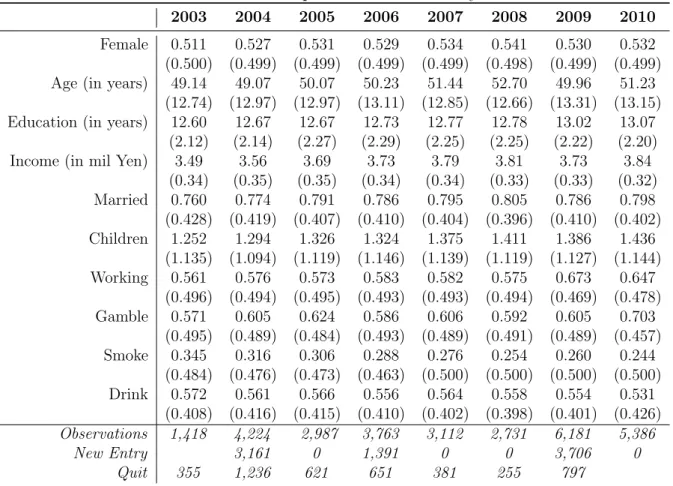
Figure 1: Variation of Declared Risk Aversion : One Year Lag ∆RA = RAt− RAt−1
Figure 2: Variation of Declared Risk Aversion : Two Years Lag ∆RA = RAt− RAt−2
Figures 1, 2, 3 and 4 display yearly, two-year, three-year and five-year variations in individual self-declared risk aversion. The solid line displays the 0 value, which represents ‘no change’ in risk aversion compared to the previous year. The dashed line shows the median value of change.13
13
If RAt= 4 and RAt−1= 4 then ∆RAt= 0. If RAt= 5 and RAt−1 = 4 then ∆RAt= 1. Therefore,
Figure 3: Variation of Declared Risk Aversion : Three Years Lag ∆RA = RAt− RAt−3
Figure 4: Variation of Declared Risk Aversion : Five Years Lag ∆RA = RAt− RAt−5
While no variation in risk aversion level is observed for most of the respondents, around 30% of interviewees report a higher or lower level of risk aversion. Almost all years present a clear bell-shaped distribution with a median of 0, but also many interviewees reporting different risk aversion levels across the years. Nonetheless, in the first two graphs of figure
1, which present the variation in individuals’ risk preferences between 2003 and 2004 and between 2004 and 2005 respectively, the median risk aversion change is different from 0, and it is first left- and then right-shifted. So it seems that something unusual happened in 2004: people posted lower risk aversion on average in 2004.
Let us denote ∆ the difference in index between year t and year t − 1. As self-reported risk aversion has a 0-10 scale, the possible range of difference in risk aversion is from −10 to 10. The former value corresponds to an extreme risk-averse agent (SRRA = 10) becoming an extreme risk lover (SRRA = 0), while the latter value can be associated with an extreme risk-seeking individual who becomes extremely risk averse. ∆+
is a dummy for becoming more risk averse: an individual declares a higher risk aversion score at year t compared to year t − 1. ∆− is a dummy for becoming less risk averse: an
individual declares a lower level of risk aversion at year t compared to year t − 1. These two dummies take value 1 only when the difference in the annual risk aversion index is greater than or equal to 2 in order to avoid respondent measurement error noise. Table
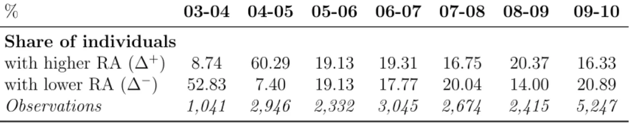
7 reports the share of individuals who declare a different level of risk aversion from one year to the next.14
Leaving aside 2003-2004 and 2004-2005, we note that around 15% and 20% of respondents declare a higher level of risk aversion than the previous year, and a similar share of the sample declare a lower level of risk aversion than in the previous survey wave.
Table 7: Yearly Change in Individuals’ Self-Reported Risk Aversion % 03-04 04-05 05-06 06-07 07-08 08-09 09-10 Share of individuals with higher RA (∆+ ) 8.74 60.29 19.13 19.31 16.75 20.37 16.33 with lower RA (∆−) 52.83 7.40 19.13 17.77 20.04 14.00 20.89 Observations 1,041 2,946 2,332 3,045 2,674 2,415 5,247
Note: 2004 refers to the variation between 2003 and 2004.
These figures provide some initial evidence that individual risk aversion may vary over time, which is at odds with the risk stability assumption commonly used. To confirm that the observed instability is really capturing actual changes in individual characteristics and not just measurement error, we investigate the relation between the yearly changes in self-declared risk aversion and shocks (such as job loss, income changes and health optimism) faced by individuals in the previous year. Such shocks could actually explain the change in declared risk aversion from one year to the next.
4.3
Is the variation in risk aversion correlated with shocks?
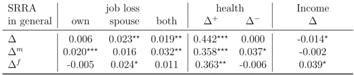
Table 8 presents the pairwise correlation matrix for changes in risk aversion and shocks. We compare changes in self-reported risk aversion with various shocks. As previously, ∆ stands for the difference in the index between year t and t − 1. Job loss is a dummy
14
We only look at the variations for participants who stay two years in a row. That is why the number of observations is less than the full sample size. In 2004, for example, we could only observe 1, 041 participants who were in the 2003 wave even though the total 2004 sample size was 4,224.
variable created if the individual, his spouse, or both have lost their job between year t and t − 1. As health variables are collected as index variables15
, we also created dummies for positive/negative changes. Personal job loss is not really significant to the SRRA, but spouse job loss is. When a spouse has lost his or her job (or both have lost their jobs), the individual declares a higher risk aversion level. When individuals are more anxious about their health, they also declare a higher risk aversion level. When it comes to income variation, we can observe a significant correlation between difference in income and change in SRRA. If the individual earns more income compared to the previous year, s/he becomes less risk averse, which is consistent with the wealth effect in the risk aversion literature. We then look at the sub-sample analyses between men and women. Men become more risk averse when they lose their own job, whereas women are more influenced by their spouses job loss. Moreover, women are more sensitive to an income change: if they become richer, they are less risk averse, while men are not influenced very much by an income change. In order to see the clearer correlation and even the underlying causation, we conduct the Mundlak random-effects model.
Table 8: Pairwise Correlation between Changes in Risk aversion and Shocks
SRRA job loss health Income
in general own spouse both ∆+
∆− ∆
∆ 0.006 0.023⋆⋆ 0.019⋆⋆ 0.442⋆⋆⋆ 0.000 -0.014⋆ ∆m 0.020⋆⋆⋆ 0.016 0.032⋆⋆ 0.358⋆⋆⋆ 0.037⋆ -0.002 ∆f -0.005 0.024⋆ 0.011 0.363⋆⋆ -0.006 0.039⋆
Notes: ⋆ 10%,⋆⋆ 5% and⋆⋆⋆ 1% significance.
∆+
refers to a positive change, ∆− refers to a negative change.
Positive change means that the individual becomes more risk averse.
∆m refers to changes for male respondents only, ∆f for female respondents only.
15
A question regarding health status is asked: “Are you anxious about your health?”. Respondents answered on a scale of 1 (absolutely agree) to 5 (do not agree at all).
4.4
Does the time-variant dimension represent a large share of
risk aversion?
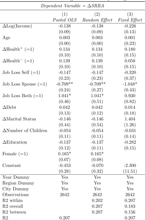
We first estimate the regression on the yearly change in risk aversion with shocks. As seen above, the change in risk aversion is correlated with income, health, and employment shocks. In addition, we control for changes in debt, marital status, having a child, and education. For the analyses, we introduce regional and year dummies in consideration of the Japanese earthquakes.16
Table 9 presents the result of delta-delta regression. Column (1) shows the estimates for the pooled OLS, and Column (2) presents the random effect model, followed by Column (3) with the fixed effect model. The yearly change in log income is negatively correlated with the change in risk aversion; the richer the individual, the less risk averse s/he becomes. Being more anxious about health also raises the risk aversion level, while being less anxious about health is relatively less clear (but has the negative sign for the fixed effect model). Those in their early 20s might change their education level. The change in education level is negatively correlated with the change in risk aversion; the more educated an individual, the less risk averse s/he becomes. This result could suggest that higher education (tertiary education) may reduce the risk aversion level. The concern is that there are not enough yearly changes to capture the correlations between the changes in risk aversion and other shocks, as the sample size is small and the panel is relatively short. We therefore use another method, the ‘Mundlak model’, to capture the time-variant and time-invariant factors in the following section.
16
In 2003-2010, there were three regional earthquakes causing more than ten casualties. The Chuetsu earthquake occurred on October 23, 2004, causing 40 casualties in the Tohoku, Hokuriku, and Kanto regions. On July 16, 2007, another Chuetsu offshore earthquake occurred with 11 casualties in the Hokuriku region. More recently, in the Touhoku region, the Iwate-Miyagi Nairiku earthquake (June 14, 2008) caused 12 casualties. We first control for those who were in the regions affected by these earthquakes at the time by introducing dummies one year after the earthquakes. However, as we control for the regions and year, the specific regions in the specific year do not give rise to any significant impact on the yearly change in individual risk aversion.
Table 9: Delta - Delta Regression on Yearly Changes
Dependent Variable = ∆SRRA
(1) (2) (3)
Pooled OLS Random Effect Fixed Effect
∆Log(Income) -0.138 -0.138 -0.226 (0.09) (0.09) (0.13) Age 0.003 0.003 0.001 (0.00) (0.00) (0.23) ∆Health+ (=1) 0.134 0.134 0.180 (0.10) (0.10) (0.15) ∆Health− (=1) 0.139 0.139 0.058 (0.10) (0.10) (0.15)
Job Loss Self (=1) -0.147 -0.147 -0.320
(0.23) (0.23) (0.37)
Job Loss Spouse (=1) -0.709** -0.709** -1.048*
(0.24) (0.27) (0.43)
Job Loss Both (=1) 1.041* 1.041* 0.930
(0.46) (0.51) (0.82) ∆Debt 0.042 0.042 0.014 (0.13) (0.12) (0.18) ∆Marital Status -0.146 -0.146 1.404 (0.44) (0.54) (1.26) ∆Number of Children -0.054 -0.054 -0.031 (0.11) (0.11) (0.14) ∆Education -0.137 -0.137 -0.282 (0.12) (0.11) (0.15) Female (=1) 0.165* 0.165* (0.07) (0.08) Constant -0.453 -0.070 -2.300 (0.28) (0.32) (11.51)
Year Dummy Yes Yes Yes
Region Dummy Yes Yes Yes
City Dummy Yes Yes Yes
Observations 2642 2642 2642
R2 within 0.202 0.207
R2 overall 0.207 0.183
R2 between 0.207 0.156
R2 0.207 0.207
Notes: ⋆ 10%,⋆⋆ 5% and⋆⋆⋆ 1% significance.
Standard errors are clustered at the individual level.
Correlated Random Effects (Mundlak, 1978) We build a statistical model in keeping with Sahm (2008), which formulates the risk aversion function RAit= xitβ+ ai to disentangle the time-variant factors xit and the time-invariant factors ai. We can model the relationship between time-invariant factor ai and the observable panel average
¯
xi as ai = ¯xiλ+ ui. We assume ui| ¯xi ∼ N (0, σu2). This approach takes up the correlated random-effects model byMundlak(1978). Also, given that our self-reported risk aversion measure is on a scale of 0 to10, we can assign a latent variable such that:
RAit = xitβ+ ¯xiλ+ ui+ ǫit
SRRAit = j, if RAj < RAit < RAj (i = 1, ..., N ; t = 1, ...T )
SRRAit is the self-reported category reported by an interviewee. By rearranging the above equation, we can exhibit the within- and between-individual variations in the risk aversion function.
RAit = (xit− ¯xi)β + ¯xi(λ + β) + ui+ ǫit (1)
RAit: Self-Reported Risk Aversion Category at time t of individual i
xit− ¯xi: Income variation, Age variation, Health shock, Employment variation, Debt Varia-tion, Marital change, Change in the number of children, Employment status change, and Education variation
¯
xi: Panel average of Log income, Age, Health, Employment, Debt, Marital status, Number of children, and Number of years of schooling
We test the impact of the panel average of time-variant variables for the same in-dividual in order to track the between-subject effect and the impact of the current variation (difference between the current variable and the panel average) to check the within-individual effect on the risk aversion parameter. To be more precise, the first term (xit− ¯xi)β captures a change in the risk aversion parameter for a given individual (within-individual variation) and the second term ¯xi(λ + β) gives the between-individual variation. We use the random-effects regression to estimate the parameters.
Table 10 presents the result of the withbetween analyses. The result across in-dividuals (between-individual variation) shows that women declare higher self-reported
risk aversion, as expected. Also, being employed is negatively correlated with the risk aversion measure.17
Table 10: Risk Aversion with Within and Between Variations : Mundlak Model Dependent Variable = Log(SRRA)
(1) (2) (1) (2)
Pooled OLS Random Effect Pooled OLS Random Effect
Within Variation Between Variation
Variation Log(Income) -0.043*** -0.037*** Mean Log(Income) -0.011 -0.026
(0.01) (0.01) (0.04) (0.04)
Variation Age -0.006 -0.006 Mean Age 0.003*** 0.003***
(0.00) (0.00) (0.00) (0.00)
Variation Health Status 0.006 0.006 Mean Health Status 0.036*** 0.030***
(0.01) (0.01) (0.01) (0.01)
Variation Employment Status Self (=1) -0.017 -0.007 Mean Employment Self -0.076*** -0.066**
(0.02) (0.02) (0.02) (0.02)
Variation Employment Status Spouse (=1) -0.016 -0.011 Mean Employment Spouse 0.095*** 0.081***
(0.02) (0.02) (0.02) (0.02)
Variation Debt 0.002 -0.002 Mean Debt -0.009 -0.006
(0.02) (0.02) (0.01) (0.01)
Variation Marital Status 0.009 0.011 Mean Marital Status -0.066* -0.060*
(0.07) (0.06) (0.03) (0.03)
Variation Number of Children -0.008 -0.009 Mean Number of Children -0.017** -0.013*
(0.01) (0.01) (0.01) (0.01)
Variation Education -0.032 -0.023 Mean Education -0.020** -0.019**
(0.02) (0.02) (0.01) (0.01)
Constant 1.157* 1.950*** Female (=1) 0.039** 0.049***
(0.58) (0.56) (0.01) (0.01)
Year Dummy Yes Yes
Region Dummy Yes Yes
City Dummy Yes Yes
Observations 8400 8400
R2 within 0.278
R2 overall 0.214
R2 between 0.175
R2 0.215
Notes: ⋆10%,⋆⋆5% and⋆⋆⋆1% significance. Standard errors are clustered at the individual level. Mean Variable is the panel average for one individual.
Variable Variation is the difference between current value and panel average.
Column (1) presents the pooled OLS on log of self-reported risk aversion and Column (2) presents the random effect model on log of self-reported risk aversion.18
The risk aversion measure shows that individuals become less risk averse when they get richer, as the log income variation is negatively correlated with the risk aversion measure with strong significance. On the other hand, age variation is positively correlated with risk aversion, meaning that when an individual gets older, s/he becomes more risk averse. If either the individual or the spouse loses his or her job, then s/he becomes more risk averse
17
Employment status: being unemployed takes the value of 0, and being employed takes the value of 1.
18
Using a logarithm means that we can obtain the percentage change in risk aversion associated with the different variables. An income change lowers risk aversion by 3.6% - 4.3% , whereas getting one year older increases risk aversion by 0.6%. Also, being a woman increases risk aversion by 3.9% - 4.9% and being anxious about health status significantly raises the risk aversion measure by 3.1% - 3.7%.
(negative correlation with a positive employment status change). Where the individual gets a higher education (tertiary education), s/he becomes less risk averse (negative correlation).19
However, these latter relations are not statistically significant. Across individuals, women and older people are more risk averse, as expected.20
Those who have concerns about their health status tend to declare a higher risk aversion level. Education is negatively correlated with risk aversion, and those who are indebted are less risk averse, and vice versa, i.e. risk-averse individuals do not like debt. Married individuals declare lower risk aversion.
Robustness Checks We observe a big shift in Risk Aversion between 2003 and 2004, raising a measurement error concern. We therefore conduct the robustness checks for our analyses without the years 2003 and 2004. Table 11 presents the result of a delta-delta regression excluding 2003 and 2004. It does not find a large difference compared to Table 9except that now the change in income in the fixed effect model gives significant effect. Table 12 presents the Mundlak model excluding the years 2003-2004. The result shows that the income and education variations reduce the risk aversion level, with slight changes in the coefficients. Therefore, we can safely say that the income change is indeed negatively correlated with risk aversion in terms of within-individual variation. Across individuals, the richer, healthier and employed men are less risk averse.
19
We have individuals aged 20-25 to be able to capture the changes in education. In Japan, individuals attend higher education in their early-to-mid 20s.
20
Table 11: Delta - Delta Regression on Yearly Changes, 2005-2010
Dependent Variable = ∆SRRA
(1) (2) (3)
Pooled OLS Random Effect Fixed Effect
∆Log(Income) -0.161 -0.161 -0.251* (0.10) (0.09) (0.13) Age 0.001 0.001 0.003 (0.00) (0.00) (0.24) ∆Health+ (=1) 0.157 0.157 0.233 (0.10) (0.10) (0.15) ∆Health− (=1) 0.144 0.144 0.058 (0.10) (0.10) (0.15)
Job Loss Self (=1) -0.141 -0.141 -0.336
(0.24) (0.23) (0.37)
Job Loss Spouse (=1) -0.644** -0.644* -0.928*
(0.25) (0.27) (0.44)
Job Loss Both (=1) 1.047* 1.047* 1.005
(0.46) (0.51) (0.82) ∆Debt 0.040 0.040 0.100 (0.14) (0.12) (0.18) ∆Marital Status 0.039 0.039 1.311 (0.40) (0.55) (1.22) ∆Child -0.125 -0.125 -0.096 (0.11) (0.11) (0.14) ∆Education -0.122 -0.122 -0.266 (0.13) (0.11) (0.15) Female (=1) 0.213** 0.213* (0.07) (0.08) Constant 1.978*** -0.119 -0.527 (0.31) (0.32) (12.82)
Year Dummy Yes Yes Yes
Region Dummy Yes Yes Yes
City Dummy Yes Yes Yes
Observations 2515 2515 2515
R2 within 0.181 0.187
R2 overall 0.176 0.146
R2 between 0.162 0.110
R2 0.176 0.187
Notes: ⋆ 10%,⋆⋆ 5% and⋆⋆⋆ 1% significance.
Table 12: Risk Aversion with Within and Between Variations : Mundlak Model, 2005-2010
Dependent Variable = Log(SRRA)
(1) (2) (1) (2)
Pooled OLS Random Effect Pooled OLS Random Effect
Within Variation Between Variation
Log(Income) -0.034*** -0.034*** Mean Log(Income) -0.024 -0.059
(0.01) (0.01) (0.04) (0.04)
Age -0.010* -0.010* Mean Age 0.003*** 0.003***
(0.00) (0.00) (0.00) (0.00)
Health Status 0.003 0.001 Mean Health Status 0.025*** 0.019**
(0.01) (0.01) (0.01) (0.01)
Employment Status Self (=1) -0.008 0.003 Mean Employment Self -0.085*** -0.069**
(0.02) (0.02) (0.02) (0.02)
Employment Status Spouse (=1) -0.006 0.001 Mean Employment Spouse 0.104*** 0.089***
(0.02) (0.02) (0.03) (0.03)
Debt 0.003 0.006 Mean Debt -0.028* -0.022
(0.02) (0.02) (0.01) (0.01)
Marital Status -0.026 -0.026 Mean Marital Status -0.037 -0.024
(0.08) (0.07) (0.03) (0.03)
Child -0.014 -0.018 Mean Number of Children -0.019** -0.014*
(0.01) (0.01) (0.01) (0.01)
Education -0.043* -0.038* Mean Education -0.013* -0.011
(0.02) (0.02) (0.01) (0.01)
Constant 1.839** 2.409*** Female (=1) 0.070*** 0.073***
(0.62) (0.58) (0.02) (0.01)
Year Dummy Yes Yes
Region Dummy Yes Yes
City Dummy Yes Yes
Observations 7235 7235
R2 within 0.007
R2 overall 0.057
R2 between 0.060
R2 0.058
Notes: ⋆10%,⋆⋆5% and⋆⋆⋆1% significance. Standard errors are clustered at the individual level. Mean Variable is the panel average for one individual.
4.5
How often should risk attitudes be collected in surveys?
Table 13and Table14present the coefficients of self-reported risk aversion when predict-ing current risky behaviors without and with socio-demographic controls, respectively. Current risky behaviors are smoking, drinking, gambling, investment in risky assets, in-debtedness, employment status, self-employment, and public sector choice. Risk aversion is negatively correlated with all the given behaviors: risk-averse individuals smoke less, drink less, gamble less, invest less in risky assets, have less debt, and fewer of them are self-employed. Using the past lagged risk aversion measures turns up fairly similar results when predicting current behaviors compared to the current risk aversion measure.
Table 13: Analyses with Past Risk-Aversion Variables on Current Behaviors
Probit estimations without controls Self Public
Smoke Drink Gamble Risky asset Debt Employed employed sector
RAt -0.080⋆⋆⋆ -0.065⋆⋆⋆ -0.071⋆⋆⋆ -0.043⋆⋆⋆ -0.032⋆⋆⋆ -0.079⋆⋆⋆ 0.003 0.016 Clustered SE (0.006) (0.007) (0.006) (0.008) (0.006) (0.006) (0.008) (0.011) Pseudo R2 0.012 0.008 0.009 0.003 0.002 0.011 0.000 0.001 observations 23,847 23,847 23,847 8,597 23,047 22,975 14,210 11,033 RAt−1 -0.081⋆⋆⋆ -0.062⋆⋆⋆ -0.065⋆⋆⋆ -0.032⋆⋆⋆ -0.033⋆⋆⋆ -0.076⋆⋆⋆ 0.001 0.011 Clustered SE (0.007) (0.008) (0.007) (0.009) (0.007) (0.007) (0.010) (0.013) Pseudo R2 0.012 0.007 0.008 0.002 0.002 0.011 0.000 0.000 observations 15,870 15,870 15,870 6,274 15,394 15,271 9,421 7,250 RAt−2 -0.086⋆⋆⋆ -0.061⋆⋆⋆ -0.067⋆⋆⋆ -0.016 -0.037⋆⋆⋆ -0.076⋆⋆⋆ 0.012 0.006 Clustered SE (0.009) (0.010) (0.009) (0.013) (0.009) (0.009) (0.013) (0.017) Pseudo R2 0.013 0.007 0.008 0.000 0.002 0.010 0.000 0.000 observations 9,476 9,476 9,476 3,215 9,183 9,075 5,558 4,246 RAt−3 -0.078⋆⋆⋆ -0.053⋆⋆⋆ -0.062⋆⋆⋆ -0.018 -0.034⋆⋆⋆ -0.075⋆⋆⋆ 0.012 0.001 Clustered SE (0.010) (0.011) (0.010) (0.016) (0.010) (0.010) (0.014) (0.018) Pseudo R2 0.011 0.006 0.007 0.001 0.002 0.011 0.000 0.000 observations 6,560 6,560 6,560 1,733 6,350 6,235 3,930 3,015 RAt−4 -0.085⋆⋆⋆ -0.062⋆⋆⋆ -0.057⋆⋆⋆ -0.011 -0.029⋆ -0.056⋆⋆⋆ -0.000 0.012 Clustered SE (0.011) (0.013) (0.011) (0.015) (0.011) (0.012) (0.016) (0.020) Pseudo R2 0.013 0.008 0.006 0.000 0.002 0.006 0.000 0.000 observations 3,962 3,962 3,962 1,738 3,840 3,732 2,418 1,874 RAt−5 -0.072⋆⋆⋆ -0.067⋆⋆⋆ -0.052⋆⋆ -0.016 -0.019 -0.031 -0.026 -0.001 Clustered SE (0.016) (0.018) (0.017) (0.018) (0.016) (0.017) (0.024) (0.030) Pseudo R2 0.009 0.009 0.005 0.000 0.001 0.002 0.001 0.000 observations 1,576 1,576 1,576 1,198 1,536 1,494 930 722 Notes: ⋆ 10%,⋆⋆ 5% and⋆⋆⋆ 1% significance.
Table 14: Analyses with Past Risk-Aversion Variables on Current Behaviors
Probit estimations with controls Self Public
Smoke Drink Gamble Risky asset Debt Employed employed sector RAt -0.034⋆⋆⋆ -0.041⋆⋆⋆ -0.055⋆⋆⋆ -0.041⋆⋆⋆ -0.017⋆ -0.042⋆⋆⋆ -0.009 0.017 Clustered SE (0.007) (0.008) (0.007) (0.009) (0.007) (0.007) (0.010) (0.013) Pseudo R2 0.195 0.082 0.046 0.068 0.092 0.177 0.075 0.047 observations 17,436 17,436 17,436 6,622 17,139 16,829 10,170 7,688 RAt−1 -0.031⋆⋆⋆ -0.038⋆⋆⋆ -0.044⋆⋆⋆ -0.036⋆⋆⋆ -0.016 -0.033⋆⋆⋆ -0.016 0.015 Clustered SE (0.009) (0.009) (0.008) (0.010) (0.008) (0.009) (0.012) (0.016) Pseudo R2 0.217 0.082 0.047 0.068 0.101 0.172 0.076 0.044 observations 11,862 11,862 11,862 4,885 11,682 11,436 6,872 5,147 RAt−2 -0.030⋆⋆ -0.037⋆⋆ -0.053⋆⋆⋆ -0.010 -0.022⋆ -0.037⋆⋆⋆ -0.007 0.010 Clustered SE (0.012) (0.012) (0.010) (0.015) (0.011) (0.011) (0.015) (0.020) Pseudo R2 0.257 0.079 0.047 0.065 0.107 0.164 0.070 0.044 observations 7,192 7,192 7,192 2,576 7,075 6,906 4,126 3,068 RAt−3 -0.024 -0.032⋆ -0.046⋆⋆⋆ -0.021 -0.021 -0.036⋆⋆ -0.013 0.007 Clustered SE (0.013) (0.013) (0.011) (0.018) (0.012) (0.012) (0.017) (0.022) Pseudo R2 0.260 0.081 0.050 0.063 0.115 0.155 0.066 0.048 observations 5,019 5,019 5,019 1,393 4,930 4,775 2,949 2,213 RAt−4 -0.037⋆⋆ -0.040⋆⋆ -0.043⋆⋆ -0.003 -0.015 -0.019 -0.023 0.022 Clustered SE (0.014) (0.015) (0.013) (0.018) (0.014) (0.015) (0.019) (0.024) Pseudo R2 0.269 0.084 0.063 0.062 0.117 0.170 0.064 0.053 observations 3,050 3,050 3,050 1,397 2,995 2,871 1,845 1,402 RAt−5 -0.048⋆ -0.055⋆⋆ -0.026 -0.006 -0.026 -0.026 -0.066⋆ -0.014 Clustered SE (0.020) (0.021) (0.020) (0.021) (0.019) (0.021) (0.028) (0.034) Pseudo R2 0.261 0.101 0.103 0.062 0.114 0.167 0.081 0.064 observations 1,237 1,237 1,237 978 1,217 1,172 730 555
Notes: ⋆10%,⋆⋆5% and⋆⋆⋆1% significance.
Control variables are gender, age, education, mother’s education, marital status and number of children.
risk aversion when predicting current risky behaviors.21
The first two rows of each table present the total average risk aversion measures: the first is panel average risk aversion over time including the current risk aversion measure, while the second excludes current risk aversion. From the third row, we calculate the average of current risk aversion at t and the past risk aversion measure at t − i where i = 1, 2, 3, 4, 5, 6.
Tables 17- Table 22show the results for the sample of individuals who appear four, five and six consecutive years. A comparison of the pseudo R2
and coefficient size shows that a four-year average provides a better prediction than the other two-year averages of risk aversion. This suggests that having more information on the time-variant dimensions of the risk aversion measure can increase explanatory power and decrease measurement noise. In addition, current behavior is more related to the recent risk aversion measures,
21
Table 15: Analyses with Average Risk-Aversion Variables on Current Behaviors
Probit estimations without controls Self Public
Smoke Drink Gamble Risky asset Debt Employed employed sector
RAPn i=0RAt−i (i+1) -0.099⋆⋆⋆ -0.082⋆⋆⋆ -0.086⋆⋆⋆ -0.047⋆⋆⋆ -0.039⋆⋆⋆ -0.095⋆⋆⋆ 0.005 0.026 Clustered SE (0.008) (0.008) (0.007) (0.009) (0.007) (0.007) (0.011) (0.014) Pseudo R2 0.015 0.011 0.011 0.003 0.002 0.013 0.000 0.001 observations 23,847 23,847 23,847 8,597 23,047 22,975 14,210 11,033 RAPn i=1RAt−i (i+1) -0.056⋆⋆⋆ -0.038⋆⋆⋆ -0.034⋆⋆⋆ -0.029⋆⋆⋆ -0.008 -0.043⋆⋆⋆ -0.002 0.011 Clustered SE (0.004) (0.004) (0.004) (0.005) (0.004) (0.004) (0.006) (0.007) Pseudo R2 0.016 0.008 0.006 0.005 0.000 0.010 0.000 0.001 observations 15,712 15,712 15,712 6,247 15,263 15,126 9,343 7,201 RAt,t−1 2 -0.111 ⋆⋆⋆ -0.084⋆⋆⋆ -0.093⋆⋆⋆ -0.052⋆⋆⋆ -0.045⋆⋆⋆ -0.106⋆⋆⋆ 0.001 0.010 Clustered SE (0.009) (0.010) (0.009) (0.010) (0.009) (0.009) (0.013) (0.017) Pseudo R2 0.016 0.010 0.012 0.004 0.003 0.015 0.000 0.000 observations 15,712 15,712 15,712 6,247 15,263 15,126 9,343 7,201 RAt,t−2 2 -0.121 ⋆⋆⋆ -0.076⋆⋆⋆ -0.091⋆⋆⋆ -0.032⋆ -0.049⋆⋆⋆ -0.109⋆⋆⋆ 0.014 0.001 Clustered SE (0.012) (0.013) (0.011) (0.015) (0.012) (0.012) (0.017) (0.022) Pseudo R2 0.019 0.008 0.011 0.001 0.003 0.015 0.000 0.000 observations 9,367 9,367 9,367 3,198 9,093 8,974 5,500 4,209 RAt,t−3 2 -0.113 ⋆⋆⋆ -0.073⋆⋆⋆ -0.079⋆⋆⋆ -0.028 -0.047⋆⋆⋆ -0.107⋆⋆⋆ 0.015 -0.007 Clustered SE (0.013) (0.014) (0.012) (0.018) (0.013) (0.013) (0.018) (0.023) Pseudo R2 0.016 0.007 0.008 0.001 0.003 0.015 0.000 0.000 observations 6,478 6,478 6,478 1,725 6,282 6,158 3,884 2,985 RAt,t−4 2 -0.123 ⋆⋆⋆ -0.079⋆⋆⋆ -0.075⋆⋆⋆ -0.021 -0.040⋆⋆ -0.091⋆⋆⋆ -0.001 0.001 Clustered SE (0.015) (0.016) (0.014) (0.018) (0.015) (0.015) (0.020) (0.026) Pseudo R2 0.019 0.008 0.007 0.001 0.002 0.010 0.000 0.000 observations 3,912 3,912 3,912 1,730 3,799 3,686 2,390 1,854 RAt,t−5 2 -0.105 ⋆⋆⋆ -0.091⋆⋆⋆ -0.075⋆⋆⋆ -0.038 -0.039⋆ -0.066⋆⋆ -0.012 -0.018 Clustered SE (0.020) (0.022) (0.020) (0.022) (0.020) (0.020) (0.028) (0.036) Pseudo R2 0.014 0.011 0.007 0.002 0.002 0.005 0.000 0.000 observations 1,556 1,556 1,556 1,193 1,518 1,476 919 714
Notes: ⋆10%,⋆⋆5% and⋆⋆⋆1% significance.
since risk aversion measured two years previously can still predict current behavior well. For this reason, collecting risk aversion every two years would definitely raise the quality of the use of the risk aversion measure in surveys. Alternatively, collecting the risk aversion measure at least every two years provides for a valid analysis, as past risk aversion at t− 2 predicts current behavior well.
Table 16: Analyses with Average Risk-Aversion Variables on Current Behaviors
Probit estimations with controls Self Public
Smoke Drink Gamble Risky asset Debt Employed employed sector RAPn i=0RAt−i (i+1) -0.041⋆⋆⋆ -0.052⋆⋆⋆ -0.065⋆⋆⋆ -0.046⋆⋆⋆ -0.017 -0.045⋆⋆⋆ -0.013 0.031 Clustered SE (0.009) (0.010) (0.009) (0.011) (0.009) (0.009) (0.013) (0.016) Pseudo R2 0.195 0.083 0.046 0.068 0.092 0.177 0.075 0.047 observations 17,436 17,436 17,436 6,622 17,139 16,829 10,170 7,688 RAPn i=1RAt−i (i+1) -0.036⋆⋆⋆ -0.029⋆⋆⋆ -0.024⋆⋆⋆ -0.025⋆⋆⋆ -0.007 -0.031⋆⋆⋆ -0.002 0.014 Clustered SE (0.005) (0.005) (0.005) (0.006) (0.005) (0.005) (0.007) (0.009) Pseudo R2 0.220 0.083 0.046 0.069 0.101 0.175 0.075 0.046 observations 11,776 11,776 11,776 4,867 11,603 11,356 6,825 5,120 RAt,t−1 2 -0.044 ⋆⋆⋆ -0.056⋆⋆⋆ -0.069⋆⋆⋆ -0.055⋆⋆⋆ -0.025⋆ -0.053⋆⋆⋆ -0.019 0.012 Clustered SE (0.011) (0.012) (0.011) (0.012) (0.011) (0.011) (0.015) (0.020) Pseudo R2 0.217 0.082 0.049 0.070 0.101 0.173 0.076 0.045 observations 11,776 11,776 11,776 4,867 11,603 11,356 6,825 5,120 RAt,t−2 2 -0.050 ⋆⋆⋆ -0.047⋆⋆ -0.074⋆⋆⋆ -0.027 -0.030⋆ -0.059⋆⋆⋆ -0.008 0.003 Clustered SE (0.015) (0.016) (0.013) (0.018) (0.014) (0.014) (0.019) (0.026) Pseudo R2 0.257 0.078 0.049 0.066 0.108 0.166 0.070 0.043 observations 7,131 7,131 7,131 2,566 7,022 6,849 4,093 3,049 RAt,t−3 2 -0.043 ⋆⋆ -0.046⋆⋆ -0.059⋆⋆⋆ -0.033 -0.033⋆ -0.061⋆⋆⋆ -0.013 -0.006 Clustered SE (0.016) (0.017) (0.014) (0.022) (0.016) (0.016) (0.021) (0.028) Pseudo R2 0.261 0.081 0.050 0.064 0.116 0.157 0.065 0.048 observations 4,972 4,972 4,972 1,390 4,891 4,731 2,922 2,199 RAt,t−4 2 -0.054 ⋆⋆ -0.049⋆⋆ -0.051⋆⋆ -0.017 -0.025 -0.048⋆⋆ -0.029 0.008 Clustered SE (0.018) (0.019) (0.017) (0.022) (0.018) (0.018) (0.024) (0.031) Pseudo R2 0.269 0.083 0.063 0.063 0.117 0.170 0.061 0.052 observations 3,021 3,021 3,021 1,394 2,974 2,845 1,829 1,392 RAt,t−5 2 -0.050 ⋆ -0.063⋆ -0.033 -0.028 -0.036 -0.048 -0.041 -0.045 Clustered SE (0.025) (0.026) (0.024) (0.026) (0.024) (0.025) (0.033) (0.040) Pseudo R2 0.258 0.102 0.102 0.063 0.115 0.169 0.074 0.066 observations 1,228 1,228 1,228 977 1,209 1,164 725 551 Notes: ⋆ 10%,⋆⋆ 5% and⋆⋆⋆ 1% significance.