HAL Id: halshs-00673892
https://halshs.archives-ouvertes.fr/halshs-00673892
Submitted on 24 Feb 2012
HAL is a multi-disciplinary open access archive for the deposit and dissemination of sci-entific research documents, whether they are pub-lished or not. The documents may come from
L’archive ouverte pluridisciplinaire HAL, est destinée au dépôt et à la diffusion de documents scientifiques de niveau recherche, publiés ou non, émanant des établissements d’enseignement et de
Optimism, pessimism and financial bubbles
Bertrand Wigniolle
To cite this version:
Documents de Travail du
Centre d’Economie de la Sorbonne
Optimism, pessimism and financial bubbles
Bertrand WIGNIOLLE
Optimism, pessimism and …nancial bubbles
B. Wigniolle
yFebruary 2, 2012
I am grateful to Michèle Cohen, Mégléna Jéléva and Jean-Christophe Vergnaud for stimulating discussions on the RDU model. I thank the participants at the conference "New challenges for macroeconomic regulation: …nancial crisis, stabilisation policy and sustainable development", Marseille 2011, for their helpful comments, and particularly Lise Clain-Chamosset, Thomas Seegmuller and Robert Becker. This paper was also presented at the 11th SAET Conference. I thank Jean-Marc Bonnisseau for his invitation and the participants at his session for their comments.
yParis School of Economics, University of Paris 1 Pantheon-Sorbonne. Address: C.E.S.,
106-112, boulevard de l’hôpital, 75647 Paris Cedex 13, France. Tel: +33 (0)1 44 07 81 98. Email : [email protected].
Abstract:
This paper shows that it is possible to extend the scope of the exis-tence of rational bubbles when uncertainty is introduced associated with rank-dependent expected utility. This RDU assumption can be viewed as a transformation of probabilities depending on the pessimism/optimism of the agent. The results show that pessimism favors the existence of deter-ministic bubbles, when optimism may promote the existence of stochastic bubbles. Moreover, under pessimism, the RDU assumption may generate multiple bubbly equilibria. The RDU assumption also leads to new condi-tions ensuring the (absence of) Pareto-optimality of the competitive equilib-rium without bubbles. These conditions still govern the existence of bubbles. JEL classi…cation: D81, D9, G1
1
Introduction
This paper shows that the scope for the existence of rational bubbles can be extended when uncertainty and rank-dependent expected utility are intro-duced. In the framework of an overlapping generations model à la Diamond (1965), the seminal article by Tirole (1985) proves that bubbles can arise in economies for which the return on capital at steady state is below the growth rate of output. The bubbleless economy must be in a state of overaccumula-tion that corresponds to dynamic ine¢ ciency. Weil (1987) proposes a model of stochastic bubbles using the same framework as Tirole, and …nds existence conditions that are even stronger. Di¤erent authors have introduced rational bubbles in richer frameworks with endogenous growth (e. g. Grossman and Yanagawa, 1993 and Olivier, 2000). But the existence of bubbles remains linked to the same condition between the growth rate and the interest rate. As empirical observations suggest that this condition is not ful…lled in general (see Abel et alii, 1989), rational bubbles seem unlikely to arise. They may perhaps not be the pertinent explanation to understand bubble phenomena that actually are observed.
In recent contributions, Caballero and Hammour (2002) and Caballero, Farhi and Hammour (2006) obtain the existence of bubbles under less strin-gent conditions at the price of a transformation of the notion of bubble. They build an overlapping generations model with an adjustment cost to capital leading to two long-run equilibria. They interpret the equilibrium correspond-ing to a higher valuation of the capital stock as a bubbly equilibrium.
This paper intends to show that it is possible to extend the scope for the existence of rational bubbles when uncertainty is introduced associated with a rank-dependent expected utility. A simple overlapping generations model is studied in which the production technology depends on a technological shock: capital return is random. In order to have a very tractable model, there are only two possible states of the nature and the capital return may oscillate between a high and a low value. In an economy in which capital is the only asset, …nancial markets are incomplete as two states of the nature exist. The existence of a bubbly asset can make …nancial markets complete. Two types of bubbles are considered in this context. The …rst type, called
a deterministic bubble, is an asset that has the same price in both states of the nature. The second type, called a stochastic bubble, is an asset whose existence is conditional to the occurrence of a particular state of the nature. As in Weil (1987), agents form their expectations according to a self-ful…lling prophecy which assumes that the bubble will burst if the other state arises. Moreover, it is assumed that agents are endowed with a rank-dependent expected utility (RDU) function. This model has been introduced by Quig-gin (1993) and developed by Chateauneuf (1999). A general presentation can been found in Cohen and Tallon (2000). According to the RDU model, the distribution of probabilities is transformed by a probability weighting func-tion (pwf). The utility is no longer linear with respect to the probabilities of the states of nature. This assumption can be viewed as a transformation of probabilities depending on the pessimism/optimism of the agent. A pes-simistic agent will give more weight to the bad state of the nature, whereas an optimistic agent will give more weight to the good state. This assump-tion has two implicaassump-tions. Firstly, the deformaassump-tion of probabilities may lead to quantitative changes with respect to the ones obtained with the standard EU (Expected Utility) model. More precisely, our results show that pes-simism favors the existence of deterministic bubbles and of small stochastic bubbles, while optimism may promote the existence of big stochastic bub-bles. Secondly, qualitative changes may arise related to the property that the weighting of the di¤erent states can change when the associated gains are modi…ed: this property can lead to a multiplicity of bubbly equilibria.
Considering pessimistic agents in the case of a deterministic bubble, the transformation of probabilities weakens the existence conditions of a bub-ble. The interpretation is simple. By assumption, the gross capital return is greater than 1 in the good state of the nature, while it is smaller than 1 in the bad state. Investing in the bubble provides a gross return equal to 1. Agents invest in the bubble in order to be protected against the occurrence of the bad state. In the case of pessimism, they put more weight on this state and invest more in the bubble. Therefore, pessimism may support the bubble.
Considering the case of a stochastic bubble, the transformation of proba-bilities may weaken the existence conditions of a bubble. Assuming that the
existence of the bubble is conditional to the state with a low capital return, the bubble bursts if the state with a high capital return emerges. Therefore, two types of bubbly equilibria may exist, associated with a low value or a high value of the bubbly asset. If the value of the bubble is low, the state with a high capital return remains the good state for the consumer. But if the value of the bubble is high, it is possible that the state with a low capital return becomes the good state for the consumer. As the consumer assigns di¤erent weights to these two cases, two types of equilibria may exist associated with a low value or a high value of the bubble.
In the case of a high value of the bubble, optimism promotes the existence of this type of equilibrium. As the good state for the consumer corresponds to the existence of the bubble, optimistic agents assign more weight to the bubbly state and invest more in the bubble. In the end, optimism favors stochastic bubbles.
In contrast, the existence of the equilibrium with a low value of the bubble is favored by pessimism. Indeed, when the value of the bubble is low, the bubbly state is the bad state of nature for the consumer. A pessimistic agent assigns more weight to this state, which favors the existence of a bubbly equilibrium.
In the case of pessimism and stochastic bubbles, an equilibrium may exist associated with a value of the bubble such that the two states of nature lead to equal levels of consumption. Moreover, this bubbly steady state may be stable and there is convergence with oscillations. There exists an in…nity of initial conditions for the value of the bubble and the bubbly equilibrium is indeterminate. The existence of such an equilibrium is due to the "kink" in the indi¤erence curves which appears for equal levels of consumption, in the two states of nature in the RDU framework.
This result can be related to previous ones obtained in …nance literature with rank dependant utility or Choquet utility: Tallon (1997) and Epstein and Wang (1994) also obtain the existence of multiple equilibria. The origi-nality of this work is to obtain the result in a production economy with capital and a bubbly asset. Bosi and Seegmuller (2010) have also developed a frame-work in which there exists an indeterminate bubbly equilibrium. In their model, indeterminacy is due to frictions introduced via a cash-in-advance
constraint with …nancial market imperfections.
This paper successively considers di¤erent assumptions: EU preferences, RDU preferences, deterministic bubbles, and stochastic bubbles. For each case, the existence conditions of bubbles are related to the Pareto optimal-ity properties of the economy without bubbles. As expected, bubbles can only appear in an economy for which the competitive equilibrium is not Pareto optimal. For RDU preferences, the condition ensuring Pareto opti-mality also depends on the transformation of probabilities implied by the pessimism/optimism of the agents. Therefore, it cannot be reduced to a comparison between the interest rate and the growth rate of the economy. It provides an additional degree of freedom that may reconcile the existence of bubbles with parameters that are empirically relevant. The study of Pareto optimality in the paper is based particularly on previous articles that have studied Pareto optimality of allocations in overlapping generations models with stochastic shocks, such as Peled (1984), Peled and Aiyagari (1991), Wang (1993), Gottardi (1996) and Demange and Laroque (1999).
Section 2 presents the basic framework with EU preferences and a com-petitive equilibrium without bubbles. A condition ensuring the Pareto op-timality of this equilibrium is derived. Section 3 studies the existence of deterministic and stochastic bubbles in this framework. Section 4 introduces RDU preferences and derives new existence conditions for bubbles. Section 5 concludes. Appendixes are presented in Section 6
2
The basic model
2.1
The competitive equilibrium without bubbles
The basic setup is an overlapping generations model with capital accumula-tion à la Allais (1947)-Samuelson (1958)-Diamond (1965). Agents live during two periods. They supply one unit of labor in the …rst period (when young) and they are retired and consume the proceeds of their savings in the second period (when old). The number of agents in each generation is normalized to 1.
Kt 1(the capital stock results from t 1 savings) and labor Lt. In each period
t exists one competitive …rm using a linear production technology Yt= R( t)Kt 1+ wLt
Capital depreciation is completed in one period. Labor productivity is con-stant and equal to w: Capital productivity R( t) follows a random process
that depends on the state of the nature t: At each period t, t 2 f1; 2g :
State 1 occurs with probability and state 2 with probability 1 : For
t= i; i = 1; 2; R(i) will be denoted Ri and it is assumed that
R1 > 1 > R2
In each period t; t is known by agents before they make their choices.
Under perfect competition, it is straightforward that w will be the equilibrium value of the wage and R( t)the capital gross rate of return.
An agent born in t knows the state of the economy for t; but not for t + 1: ct is the …rst period consumption, st is the amount of savings, and dt+1 is
the second period consumption that is a random variable in t. The budget constraints of the agent are:
ct+ st = w (1)
dt+1 = R( t+1)st (2)
The agent is endowed with an intertemporal utility function. The utility function of a generation t agent is:
ln ct+ Etln(dt+1) (3)
Et is the expectation taken in period t: Maximizing (3) under budget
con-straints (1) and (2) gives the results: ct = w 1 + st = w 1 + dt+1 = R( t+1) w 1 +
Results do not depend on as the VNM function is logarithmic. The capital stock used in period t + 1 results from savings in t :
Kt =
w 1 +
Therefore, after one period, the capital stock reaches a constant value. In t = 0; the initial value of the capital stock K 1 is given, as the
con-sumption level of the …rst old agent: d0 = R( 0)K 1:
2.2
Pareto optimality of the competitive path
A standard result in deterministic models is that the existence of …nancial bubbles is possible only in economies that are ine¢ cient. If uncertainty is removed from the model (R(1) = R(2) = R), dynamic e¢ ciency is obtained for R > 1:
In an economy with uncertainty, the appropriate concept of Pareto opti-mality for allocation is interim optiopti-mality (see Demange and Laroque (1999)). A feasible allocation is interim optimal if no other feasible allocation exists that, almost surely, yields a higher expected utility for all periods t with a strict improvement on a set of states of positive measure.
Interim Pareto optimality can be translated in this framework as follows. Firstly, the notion of feasible path is introduced. In period t, the resource constraint of the economy can be expressed as:
ct+ dt+ Kt= R( t)Kt 1+ w (4)
A feasible path is an allocation (ct; dt; Kt)t 0;starting from a given value for
K 1; that satis…es the resource constraint (4) for all t:
Proposition 1 If
R1
+ 1 R2
< 1 (5)
the competitive equilibrium is interim Pareto optimal. Proof. See Appendix 1.
The proposition shows that interim Pareto optimality is preserved if the low value of R2 in the bad state is compensated by a high enough value
of R1 in the good state. It is interesting to note that if (5) holds, then
R1+ (1 )R2 > 1:Therefore, Pareto optimality needs a stronger condition
than an average interest rate higher than the growth rate of capital.
3
The equilibrium with …nancial bubbles
This section assumes the existence of a bubble asset. This asset is a pure bubble, with a fundamental value equal to 0. Two types of bubbles are studied: one is called a bubble "à la Tirole" which is "deterministic", while the second is a bubble "à la Weil " which is "stochastic". The deterministic bubble is a deterministic asset that has the same price in the two states of the nature. The stochastic bubble only exists in state 2 (the bad state of the nature). Its existence is therefore conditional to the continuation of this state and at each period, the bubble has a probability of exploding in the next period.
3.1
Existence of an equilibrium with a deterministic
bubble
It is assumed that a bubble asset is available in the economy in a …xed quantity normalized to 1: Its price is pt in period t: The budget constraints
of a generation t agent become:
ct+ st+ ptxt = w (6)
dt+1 = R( t+1)st+ pt+1xt (7)
Maximizing (3) under budget constraints (6) and (7) gives the results: ct = w 1 + (8) st = w 1 + 1 ptR2pt+1 1 ptR1 pt+1 1 ! (9) pt+1xt = w 1 + " (1 ) R1 ptR1 pt+1 1 R2 1 ptR2pt+1 # (10) Equilibrium conditions on the bubble and capital markets imply:
xt = 1 (11)
Kt = st (12)
Condition (11) with (10) gives the dynamics of the price of the bubble: pt+1= w 1 + " (1 ) R1 ptR1 pt+1 1 R2 1 ptR2pt+1 #
This dynamics has two steady states, 0 which is stable and a positive sta-tionary state p that is unstable:
p = w 1 + (1 ) R1 R1 1 R2 1 R2
At this stationary state, the value of savings is:
s = w
1 + 1 R2
1 R1 1
Finally, this equilibrium exists only if p and s are positive, which gives:
R1
+(1 )
R2
> 1 (13)
R1+ (1 ) R2 > 1 (14)
When the second condition (14) does not hold, it is straightforward enough to show that a bubbly equilibrium exists without investment in cap-ital. This equilibrium is associated with a constant value of the bubble:
p = w
The existence of this equilibrium is related to the assumption of a linear technology, that allows production to occur without using capital.
The results can be summarized by a proposition:
Proposition 2 If condition (13) holds, there exists an equilibrium of the economy associated with a deterministic bubble.
If (14) is satis…ed, agents hold both capital and the bubble asset at equilibrium.
If (14) is not satis…ed, a bubbly equilibrium exists with no investment in capital.
Condition (13) is the converse of the condition that ensures interim Pareto optimality of the competitive equilibrium. As expected, a bubbly equilibrium can only exist in an economy that is not interim Pareto optimal.
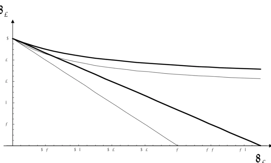
When (14) is not ful…lled, two di¤erent equilibria may exist: a …rst one with capital and no bubble, a second one without capital and with the bubbly asset. This second bubbly equilibrium Pareto-dominates the …rst one (in the sense of interim Pareto optimality). Indeed, with the bubbly equilibrium there is no risk on the gross return of the asset that is equal to 1, and 1 is higher than the expected return with the equilibrium with capital (1 > R1+
(1 ) R2). Figure 1 gives an illustration of the di¤erent cases depending on
the values of R1 and R2:The curves are drawn for the value = 1=2:
Remark 1 This paper focuses only on two types of bubbles: a deterministic one that has the same value in all states of the nature; a stochastic one that cancels out if state 1 occurs. More generally, the case of a bubbly asset that takes two positive di¤erent values depending on the state of the nature could be studied. It is easy to check that this type of solution does not exist in our framework.
3.2
Existence of an equilibrium with a stochastic
bub-ble
A bubble asset à la Weil (1987) is available in the economy in a …xed quantity normalized to 1: Its price is pt in period t; conditional to the realization of
state 2. Assuming that the economy is in period t in state 2, agents expect a price pt+1 in period t + 1 conditional to the realization of state 2, and a price
0 if state 1 occurs. In the case of the bubble exploding, the dynamics of the economy after the explosion becomes the same as in the economy without the bubble.
Assuming that state 2 occurs in period t; the budget constraints of a generation t agent are:
ct+ st+ ptxt = w (15)
d1t+1 = R1st (16)
d2t+1 = R2st+ pt+1xt (17)
where d1t+1 is the consumption level in state 1 and d2t+1 in state 2.
Maximizing (3) under budget constraints (15), (16) and (17) gives the results: ct = w 1 + st = w 1 + 1 ptR2pt+1 xt = w 1 + (1 ) pt R2 pt+1 ptR2
Equilibrium conditions on the bubble market (xt= 1) and on the capital
market Kt= st imply: 1 = w 1 + (1 ) pt R2 pt+1 ptR2 (18) Kt = w 1 + 1 ptR2pt+1 (19)
With the change of variable t = pt(1 + )=( w); equation (18) gives: t+1= R2 t
1 t
1 t
This equation has 2 stationary states: 0 which is stable, and
= 1 R2
which is unstable. This last steady state exists only if > 0,
R2 < 1 (20)
Proposition 3 If condition (20) holds, there exists an equilibrium of the economy associated with a stochastic bubble conditional to the continuation of state 2.
This condition is stronger than (13): the deterministic bubble is more likely to exist than the stochastic bubble. Indeed, the stochastic bubble has a positive return only if state 2 arises. Moreover, the stochastic bubble cannot exist in an e¢ cient economy: if (20) holds, (5) does not hold. A graphical illustration of these results is shown in Figure 1, with a value = 1=2:
4
Bubbles with a rank-dependent utility
4.1
Preferences
The agent is now endowed with an intertemporal rank-dependent expected utility (RDU) function. Following Quiggin (1993), the distribution of prob-abilities is transformed by a probability weighting function (pwf) : is a continuous increasing function from [0; 1] to [0; 1] such that (0) = 0 and
(1) = 1:
With this assumption, the preceding utility function (3) must be trans-formed according to the following rules.
Denoting c; d1 and d2; the consumption levels when young, when old in
the state 1 and old in the state 2; the utility function is: if d1 > d2;
ln c + ( ) ln(d1) + [1 ( )] ln(d2) (21) if d1 < d2;
In abbreviated form, the utility function will be denoted by:
ln c + E ln(d) (23)
where E is the expected value calculated with the transformed probabilities according to (21) and (22), and d is the random variable (d1; d2; ; 1 ) :
The property ( ) < can be interpreted as pessimism and ( ) > as optimism. An optimistic agent puts more weight on the best state of the nature, whereas a pessimistic agent puts more weight on the worst state.
The following notations will be used from now: 1 = ( ) and 2 =
1 (1 ). Therefore, for a pessimistic agent, 1 < < 2; and for an
optimistic agent 1 > > 2:
The RDU assumption has two main consequences. The …rst one corre-sponds to the deformation of probabilities, that may lead to quantitative changes: with respect to the EU model, the agents behave as if they did not take into account the true probabilities. The second consequence corre-sponds to the existence of a kink in the indi¤erence curves for d1 = d2: This property may imply qualitative change in the behaviors of the agents that choose to consume the same level in the two states of the nature for di¤erent price levels. In the literature on RDU preferences, it often generates multiple equilibria.
4.2
The equilibrium without bubbles
What is the impact of the RDU assumption on the former analysis? Con-sidering the competitive equilibrium without bubbles, it is clear that state 1 is the good state of the nature and state 2 the bad state. Therefore, the utility function is always given by (21). Moreover, the RDU assumption has no impact as the consumption choices do not depend on . Consumption and savings remain equal to
ct = w 1 + st = w 1 + dt+1 = R( t+1) w 1 +
The capital stock from t = 0 is equal to: Kt =
w 1 +
What can be said about the Pareto optimality of the equilibrium without bubbles? It is necessary to study separately the cases of pessimistic and optimistic agents. In both cases, the utility function is not di¤erentiable at a point such that d1 = d2: But, if agents are pessimistic, their preferences
remain convex, whereas this property is lost for optimistic agents. In the …rst case, it is easy to adapt the result of Proposition 1. Proposition 4 If agents are pessimistic and
1
R1
+1 1
R2
< 1 (24)
the competitive equilibrium without bubbles is interim Pareto optimal. Proof. See Appendix 2.
This condition is the same as the one of Proposition 1, except that is replaced by 1: This is due to the transformation of probabilities in the
utility function of the agent.
A condition ensuring the Pareto e¢ ciency of the competitive equilibrium without bubbles is more di¢ cult to establish when agents are optimistic, be-cause agents’preferences are no longer convex. The next proposition shows that the preceding e¢ ciency condition remains necessary. But another con-dition is needed that can be interpreted as a one of "moderate" optimism, or a weak transformation of the probabilities.
Proposition 5 Assuming optimistic agents, if
1 R1 +1 1 R2 < 1 (25) and R2 R1 < " 2 1 (1 1) (1 2) 2 2 (1 2) (1 2) # 1 1 2 (26) the competitive equilibrium without bubbles is interim Pareto optimal.
Proof. See Appendix 3.
As it is apparent in the proof, Condition (26) is needed because prefer-ences are not convex for an optimistic agent. It guarantees that no other feasible allocation dominating the competitive equilibrium exists in the zone in which d1 < d2: A better intuition can be achieved in particular cases. The
following corollary studies the limit condition obtained from (26) when the transformation of probabilities vanishes. Then, it takes a particular assump-tion for
( ) = ; with 0 < < 1 The lower ; the more optimistic the agent is.
Corollary 1 1. In the limit case 1 ! and 2 ! ; Condition (26)
becomes R2=R1 < 1, which is true by assumption. By continuity, (26)
is ful…lled if the transformation of probabilities is weak.
2. Let us assume that ( ) = with 2 (0; 1): There exists a value 2 (0; 1) such that (26) is satis…ed if and only if > :
Proof. See Appendix 4.
The …rst part of the corollary shows that Condition (26) is satis…ed in the limit case 1 ! and 2 ! : By continuity, it is satis…ed if the
transformation of probabilities is not too strong. The second part introduces a particular function that allows the transformation of probabilities to be measured by the parameter : can be interpreted as the degree of pessimism (or as the opposite of the degree of optimism). The corollary allows a lower bound on to be de…ned that represents a limit value for the degree of optimism.
4.3
Deterministic bubbles
For a deterministic bubble, it is clear that second period consumption in state 1 will always be greater than second period consumption in state 2, as:
Therefore, the analysis of Section 3.1 can be used again, replacing by 1:
A bubbly equilibrium will exist if:
1
R1
+(1 1) R2
> 1 (27)
It will be associated with a positive investment in capital if
1R1+ (1 1) R2 > 1 (28)
If (28) is not ful…lled, there exists an equilibrium in which the bubble asset is the only asset of the economy, with a price
p = w
1 + Condition (27) de…nes an upper bound on 1:
1 <
R1(1 R2)
R1 R2
The case of pessimism
Agents are assumed to be pessimistic: 1 < : If 1 <
R1(1 R2)
R1 R2
<
a deterministic bubble exists in an economy in which there would be no bubble if agents did not "transform" the probabilities. The interpretation of this result is simple. Investing in the bubble provides a gross return equal to 1;which is greater than the capital return in the bad state of the nature R2:
Agents invest in the bubble in order to be protected against the occurrence of state 2. In the case of pessimism, they put more weight on this state and invest more in the bubble. Therefore, pessimism can play in favor of the existence of a deterministic bubble. From Proposition 4, a bubbly equilibrium can only exist in an ine¢ cient economy.
Figure 2 gives an illustration of the e¤ect of pessimism on the existence of the di¤erent regimes in the plane (R1; R2):The curves are obtained under the
assumption that the pessimism generates a transformation of from = 1=2 to 1 = 0:4:
The case of optimism
The condition ensuring the existence of a bubbly equilibrium remains Con-dition (27). Optimism is unfavorable to the existence of bubbles, as agents put more weight on the good state of the nature.
The relation between the existence of bubbles and interim Pareto opti-mality is more complex in the case of optimism. The usual way to analyze the impact of a bubble is to interpret it as an intergenerational transfer. In the basic economy with standard EU preferences, when (5) is not ful…lled, the existence of a bubble constitutes an intergenerational transfer from the young to the old agents and this transfer is Pareto improving. This analysis can also be used to understand the case of pessimistic agents. But, with opti-mistic agents, preferences are no longer convex. If (25) holds and (26) is not ful…lled, it may be possible that the economy is not interim Pareto optimal and that no bubbly equilibrium exists. Considering the proof of Proposi-tion 5, the competitive equilibrium without bubbles can be ine¢ cient in this case, because the technology does not allow agents to redistribute consump-tion from state 1 in favor of state 2. A deterministic bubble cannot solve this problem as the bubble carries out a transfer among generations, and not a transfer among the two states of nature.
4.4
Stochastic bubbles
4.4.1 Two types of bubbly equilibria
A stochastic bubble conditional to state 2 may induce some redistribution of consumption between the two states of nature. For the equilibrium with a deterministic bubble, state 1 always remains the best state of the nature. For an equilibrium with a stochastic bubble conditional to state 2, it is possible that state 2 becomes the good state of the nature, as the bubble bursts in state 1. More precisely, the size of the bubble may determine which is the best state. For a small bubble, state 1 will always lead to more consumption than state 2. For a large bubble, the inequality can be reversed. Therefore, it is a priori possible to obtain two types of bubbly equilibria, associated either with d2 < d1 or with d2 > d1:
generation t agent remain the same: ct+ st+ ptxt = w
d1t+1 = R1st
d2t+1 = R2st+ pt+1xt
Equilibrium such that d2 > d1
Assuming that the equilibrium is such that d2
t+1 > d1t+1;the program of the
agent consists in maximizing (22) under the three budget constraints. The results are: ct = w 1 + st = w 1 + 2 1 ptR2pt+1 xt = w 1 + (1 2) pt 2R2 pt+1 ptR2
The equilibrium conditions lead to the dynamics of the price of the bubble. Using the variable t= pt(1 + )=( w); t follows the dynamic equation:
t+1 = R2 t
1 t
1 2 t
The bubbly steady state corresponds to
^ = 1 2 R2
1 R2
It exists only if
2 < 1 R2 (29)
Moreover, the assumption that d1 < d2 must be checked along this equilib-rium. It leads to the constraint:
2 <
1 R2
R1+ 1 R2
(30) This last condition is stronger than (29) as R1+ 1 R2 > 1.
Equilibrium such that d2 < d1
Assuming that the equilibrium is such that d2
t+1 < d1t+1; the program of
the agent gives:
ct = w 1 + st = w 1 + 1 1 ptR2pt+1 xt = w 1 + (1 1) pt 1R2 pt+1 ptR2
The variable t= pt(1 + )=( w) follows the dynamic equation: t+1 = R2 t
1 t
1 1 t
The bubbly steady state corresponds to
= 1 1 R2
1 R2
It exists only if
1 < 1 R2 (31)
Moreover, the assumption that d1 > d2 leads to the constraint that: 1 >
1 R2
R1+ 1 R2
(32) 4.4.2 Stochastic bubbles and optimism
For an optimistic agent, 1 > > 2; and thus, ^ > : Depending on the
value of the parameters, it is possible to obtain a bubbly equilibrium with d1 < d2 and a high price level of the bubble, or a bubbly equilibrium with
d1 > d2 and a low price level of the bubble.1
Using conditions (29), (30) , (31) and (32), the following results may be obtained.
Proposition 6 Assume that 2 < R1+1 R21 R2 and 1 > 1 R2 or 1 < R11 R2+1 R2:
There exists a unique bubbly equilibrium with d1 < d2 and a price of the bubble
equal to ^( w)=(1 + ):
1It is not possible to obtain a bubbly equilibrium such that d1= d2; because it is never
Proposition 6 shows that optimism can play in favor of the existence of bubbles. Assume that > 1 R2: Under this condition, stochastic bubbles
cannot exist in the economy with EU preferences. If agents are optimistic, it is possible that they transform probabilities with 2 = 1 (1 ) < R11 R2+1 R2:
In this case a stochastic bubble may exist. The price of the bubble is high enough in such a way that consumption in state 2 (the bubble exists) is higher than consumption in state 1 (the bubble explodes). As agents are optimistic, they put more weight on the good state and invest more in the bubble.
Proposition 7 corresponds to the converse case of a low price of the bubble such that d1 remains higher than d2:
Proposition 7 Assume that 1 < 1 R2 and 2 > R1+1 R21 R2 : There exists
a unique bubbly equilibrium with d1 > d2 and a price of the bubble equal to
( w)=(1 + ):
As < 1 < 1 R2; a necessary condition for the existence of such
an equilibrium is that there exists a bubbly equilibrium in the economy with EU preferences (see condition (20)). Moreover agents need to be not too opti-mistic, in such a way that 1and 2remain in the interval R11 R2+1 R2; 1 R2 :
A last case remains to be studied, if
2 <
1 R2
R1+ 1 R2
< 1 < 1 R2
In this case, all preceding conditions (29), (30) , (31) and (32) are ful…lled. But, it does not imply that the two types of bubbly equilibria can exist together. Indeed, in the case of optimistic agents, preferences are not convex. It is possible that two di¤erent solutions satisfy the marginal conditions of the consumer program, one with d1 < d2, the other one with d1 > d2: Therefore, it is necessary to compare the utility levels associated with the two solutions. This is done in the following proposition.
Proposition 8 The function is de…ned according to:
( ) = ln R1
1 R2
Assuming
2 <
1 R2
R1+ 1 R2
< 1 < 1 R2
there exists two cases:
If ( 2) > ( 1) then a bubbly equilibrium with d1 < d2 exists and the
price of the bubble is equal to ^( w)=(1 + ):
If ( 2) < ( 1) then a bubbly equilibrium with d1 > d2 exists and the
price of the bubble is equal to ( w)=(1 + ): Proof. See Appendix 5.
To summarize the impact of optimism on the existence of stochastic bub-bles, the most interesting result is obtained in Proposition 6. Optimism may favor stochastic bubbles with respect to EU preferences. The price of the bubble must be high enough in such a way that d1 < d2:In that case, state 2
(the bubble exists) can be better than state 1 (the bubble bursts). Optimistic agents put more weight on the good state and invest more in the bubble. 4.4.3 Stochastic bubbles and pessimism
For a pessimistic agent, 1 < < 2: The preceding conditions (29), (30),
(31) and (32) allow existence conditions for the bubbly equilibria to be ob-tained that satisfy the marginal conditions of the consumer program. But, in the case of pessimism, another situation may exist that corresponds to d1
t+1 = d2t+1. This case results from the existence of a kink for d1t+1 = d2t+1:
Considering the maximization of the RDU function under the intertempo-ral budget constraint (39), the optimal solution with d1
t+1= d2t+1 is obtained if: 1 1 1 < 1 R2pt+1pt R1pt+1pt < 2 1 2
It corresponds to the solution: ct = w 1 + d1t+1 = d2t+1 = w 1+ 1 R1 R2 R1 pt pt+1 + pt pt+1
The equilibrium price of the bubble satis…es: pt= w 1 + pt pt+1(R1 R2) 1 + pt+1pt (R1 R2)
With the change of variable t = pt(1 + )=( w); this equation gives: t = 0 or
t+1 = t(R1 R2) + (R1 R2) (33)
(33) has a stationary state
~ = R1 R2
1 + R1 R2
If R1 R2 > 1;this stationary state is unstable. If R1 R2 < 1;it is stable. In
this case, it is possible to observe convergence towards the stationary state, with oscillations. In the case of instability, there is only one stationary bubbly equilibrium. In the case of stability, a multiplicity of bubbly equilibria exists. Finally, the following results have been obtained in the case of a pes-simistic agent:
Proposition 9 Assume that 1 < < 2:
If
2 <
1 R2
R1+ 1 R2
a bubbly equilibrium with d1 < d2 exists and the price of the bubble is
equal to ^( w)=(1 + ): If
1 R2
R1+ 1 R2
< 1 < 1 R2
a bubbly equilibrium with d1 > d2 exists and the price of the bubble is
equal to ( w)=(1 + ): If 1 < 1 R2 R1 + 1 R2 < 2
a stationary bubbly equilibrium exists associated with a price of the bubble ~( w)=(1 + ):
- If R1 R2 > 1; this stationary state is unstable.
- If R1 R2 < 1; it is stable. In this case, a multiplicity of bubbly
equilibria exists that converge towards the steady state with oscil-lations.
To summarize, pessimism may favor stochastic bubbles such that d1 >
d2 with respect to EU preferences. To illustrate this point, assume that
> 1 R2: Under this condition, stochastic bubbles cannot exist in the
economy with EU preferences. If agents are pessimistic, it is possible that they transform probabilities in such a way that 1 = ( ) < 1 R2: In this
case a stochastic bubble can exist. The price of the bubble is low enough in such a way that consumption in state 2 (the bubble exists) remains lower than consumption in state 1 (the bubble explodes). As agents are pessimistic, they put more weight on the bad state and invest more in the bubble.
Moreover it is possible to have indeterminacy with a multiplicity of bubbly equilibria converging towards a steady state with oscillations. This result of indeterminacy is related to the existence of a kink on the indi¤erence curves for d1 = d2. When d1 = d2; it is possible that di¤erent values of the
price of the bubble are compatible with an equilibrium. Similar results have been obtained with RDU preferences or Choquet utility in other frameworks: Tallon (1997) and Epstein and Wang (1994) also demonstrate the existence of multiple equilibria in models of …nancial assets.
5
Conclusion
This paper has proposed a simple model that suggests that uncertainty as-sociated with RDU preferences can extend the scope for the existence of rational …nancial bubbles. Pessimism favors the existence of deterministic bubbles, when optimism may promote the existence of stochastic bubbles. Moreover, associated with pessimism, the RDU assumption is a new cause of multiple bubbly equilibria.
It would be interesting to expand these …rst results into a more gen-eral framework. A …rst improvement would consist in introducing di¤erent
production technologies subject to di¤erent shocks, with many states of the nature. Considering non-linear production technologies could also be an in-teresting generalization.
Another development would be to assume heterogeneous agents di¤ering by their degree of pessimism or optimism.
References
[1] Abel, Andrew B, N. Gregory Mankiw, Lawrence H. Summers and Richard J. Zeckhauser, 1989. "Assessing Dynamic E¢ ciency: Theory and Evidence," Review of Economic Studies, Wiley Blackwell, vol. 56(1), pages 1-19, January.
[2] Allais, Maurice, Economie et intérêt, ed. Imprimerie Nationale, 1947 [3] Bosi, Stefano and Thomas Seegmuller, On rational exuberance,
Mathe-matical Social Sciences, Volume 59, Issue 2, March 2010, Pages 249-270 [4] Ricardo J. Caballero & Mohamad L. Hammour, 2002. "Speculative Growth," NBER Working Papers 9381, National Bureau of Economic Research, Inc.
[5] Caballero, Ricardo J., Emmanuel Farhi and Mohamad Hammour, 2006, Speculative Growth: Hints from the U.S. Economy, American Economic Review, vol 96(4): 1159-1192.
[6] Chateauneuf, A. ”Comonotonicity axioms and RDU theory for arbitrary consequences”, Journal of Mathematical Economics, 32, 21-45, 1999. [7] Cohen, M. and J M Tallon, "Décision dans le risque et l’incertain:
l’apport des modèles non-additifs", Revue d’Economie Politique, N 110(5), 2000, pp.631-681.
[8] De La Croix, David and Philippe Michel, A theory of economic growth: dynamics and policy in overlapping generations, Cambridge University Press; (2002).
[9] Demange, Gabrielle and Guy Laroque, Social Security and Demographic Shocks, Econometrica, Vol. 67, No. 3 (May, 1999), pp. 527-542
[10] Diamond, Peter, 1965, National Debt in a Neoclassical Growth Model, American Economic Review, vol 55(5): 1126–50.
[11] Dow, James & da Costa Werlang, Sergio Ribeiro, 1992. "Excess volatility of stock prices and Knightian uncertainty," European Economic Review, Elsevier, vol. 36(2-3), pages 631-638, April.
[12] Larry G. Epstein and Tan Wang, Intertemporal Asset Pricing under Knightian Uncertainty, Econometrica, Vol. 62, No. 2 (Mar., 1994), pp. 283-322
[13] Piero Gottardi, Stationary Monetary Equilibria in Overlapping Genera-tions Models with Incomplete Markets, Journal of Economic Theory 71, 75 89 (1996).
[14] Grossman, Gene and Noriyuki Yanagawa, 1993, Asset Bubbles and En-dogenous Growth, Journal of Monetary Economics, vol 31(1): 3-19. [15] Homburg, Stefan. E¢ cient Economic Growth. Berlin usw. Springer,
1992.
[16] Olivier, Jacques, 2000, Growth-enhancing Bubbles, International Eco-nomic Review, vol 41(1): 133-151.
[17] Peled, Dan, Stationary Pareto Optimality of Stochastic Asset Equilibria with Overlapping Generations, Journal of Economic Theory 34, 396-403 (1984).
[18] Peled, Dan, and Rao Aiyagari, Dominant Root Characterization of Pareto Optimality and the Existence of Optimal Equilibria in Stochas-tic Overlapping Generations Models, Journal of Economic Theory 54, 69-83 (1991).
[19] Quiggin, J. ”A theory of anticipated utility”,Journal of Economic Be-havior and Organisation, 3, p. 323–343, 1982.
[20] Samuelson, Paul, 1958, An Exact Consumption-Loan Model of Interest with or without the Social Contrivance of Money, Journal of Political Economy, vol 66: 467-482.
[21] Tallon, J M, Risque microéconomique et prix d’actifs dans un modèle d’équilibre général avec espérance d’utilité dépendante du rang Finance, Revue de l’Association Française de Finance, N 18, 1997, pp. 139-153. [22] Tirole, Jean (1985): “Asset Bubbles and Overlapping Generations,”
Econometrica, 53(6), 1499-1528.
[23] Wang, Y. (1993): "Stationary Equilibria in an Overlapping Generations Economy with Stochastic Production," Journal of Economic Theory, 61, 423-435.
[24] Weil, Philippe, 1987, Con…dence in the Real Value of Money in an Overlapping Generations Economy, Quarterly Journal of Economics, vol 52(1): 1-22.
6
Appendixes
6.1
Appendix 1
Proof of Proposition 1.
The proof uses the method developed by Homburg (1992) and De la Croix and Michel (2002). For the proof, it is useful to introduce some notations. ht denotes a particular history from period 0 till t (the state 0 at period
0 is assumed to be known in t = 0): ht = ( 0; 1; 2; :::; t): Ht is the set
of all possible t-period histories from period 0: #Ht = 2t as 0 is known
in 0. The applications and are de…ned such that, for an history ht =
( 0; 1; 2; :::; t 1; t) 2 Ht; (ht) = ( 0; 1; 2; :::; t 1) and (ht) = t:
for all t 0: K 1 is given d0 = R( 0)K 1 ct = w 1 + c Kt = w 1 + K dt+1 = R( t+1) w 1 + Using the following notation,
d( t) =
R( t) w
1 + the corresponding ex-ante utility level is:
U ln (c) + ln d(1) + (1 ) ln d(2)
Assuming that this allocation is not interim Pareto optimal means that there exists another feasible allocation that, almost surely, gives a higher expected utility for all period t with a strict improvement on a set of states of positive measure. Formally, it means that it is possible to …nd an allocation (~c(ht); ~d(ht); ~K(ht))ht2Ht; t 0 such that 8t
~
c(ht) + ~d(ht) + ~K(ht) = R( (ht)) ~K( (ht)) + w
~
K ( (h0)) = K 1 (initial condition given)
(feasibility), and such that 8t; 8ht 2 Ht
ln (~c(ht)) + ln d((h~ t; 1)) + (1 ) ln d((h~ t; 2)) U (34)
~
d( 0) R( 0)K0(35)
with a strict inequality for some ht0:
First, it is easy to check that the competitive solution (c; d(1); d(2)) in period t can be obtained through the following program:
max (c;d1;d2)ln (c) + ln d 1 + (1 ) ln d2 s.t. w = c + R1 d1+ (1 ) R2 d2
As a consequence of this property, (34) implies that, 8t; 8ht2 Ht ~ c(ht) + R1 ~ d((ht; 1)) + (1 ) R2 ~ d((ht; 2)) c + R1 d(1) + (1 ) R2 d(2) with a strict inequality for some history ht0:
For a state t; t2 f1; 2g ; the function is de…ned as:
(1) = (2) = 1
For an history ht = ( 0; 1; 2; :::; t 1; t) 2 Ht; P (ht)is de…ned as
P (ht) = t Q i=1 ( i) t Q i=1 R( i) and P ( 0) = 1: Therefore, P (ht) = ( (ht)) R( (ht)) P ( (ht))
For T > t0; it is obtained that
~ d( 0) d0+ TP1 t=0 P ht2Ht P (ht) ~c(ht) + R1 ~ d((ht; 1)) + (1 ) R2 ~ d((ht; 2)) c R1 d(1) (1 ) R2 d(2) > 0 Rearranging the terms that depend on the same period, the following is
obtained: TP1 t=0 P ht2Ht P (ht) h ~ c(ht) + ~d(ht) c d( (ht)) i + P hT2HT P (hT) h ~ d((hT)) d( (hT)) i > 0 From the feasibility constraints, it is obtained:
TP1 t=0 P ht2Ht P (ht) h R( (ht)) ~K( (ht)) K(h~ t) R( (ht))K + K i + P hT2HT P (hT) h ~ d((hT)) d( (hT)) i > 0
After simpli…cations, it is obtained: P hT 12HT 1 P (hT 1) h ~ K(hT 1) + K i + P hT2HT P (hT) h ~ d((hT)) d( (hT)) i > 0 (36) It is possible to write: ~ K(hT 1)+K = R(1)R(1) h ~ K(hT 1) + K i +1 R(2)R(2) h ~ K(hT 1) + K i Replacing in (36) makes it possible to write:
P hT2HT P (hT) h ~ d(hT) R( (hT)) ~K ( (hT)) d( (hT)) + R( (hT))K i > 0 Using the feasibility constraint leads to:
P hT2HT P (hT) h c + K c(h~ T) K (h~ T) i > 0 Finally, c + K = w and it is obtained:
" P hT2HT P (hT) # w > P hT2HT P (hT) h c + K ~c(hT) K (h~ T) i > 0 Introducing the notation
ST =
P
hT2HT
P (hT)
it is straightforward to check that ST = R1 +1 R2 ST 1 Therefore, if R1 + 1R2 < 1; lim
T !1ST = 0 and the competitive equilibrium is
interim Pareto-optimal.
6.2
Appendix 2
The proof is adapted from the preceding one, replacing by 1. The
com-petitive solution in period t can be obtained through the following program: max (c;d1;d2)ln (c) + 1ln d 1 + (1 1) ln d2 s.t. w = c + 1 R1 d1+(1 1) R2 d2
As the agent is pessimistic, its preferences remain strictly convex. There-fore, the preceding reasoning can be used: a feasible allocation (~c(ht); ~d(ht);
~
K(ht))ht2Ht; t 0 that interim Pareto-dominates the competitive equilibrium
must satisfy 8t; 8ht2 Ht ~ c(ht) + 1 R1 ~ d((ht; 1)) + (1 1) R2 ~ d((ht; 2)) c + 1 R1 d(1) + (1 1) R2 d(2) with a strict inequality for some history ht0:Thereafter, the proof is the same,
replacing by 1:
6.3
Appendix 3
The proof is adapted from Appendix 1. The competitive solution in period t can be obtained through the following program:
max (c;d1;d2)ln (c) + 1ln d 1 + (1 1) ln d2 s.t. w = c + 1 R1 d1+(1 1) R2 d2
But, as the agent is optimistic, its preferences are no more convex. More precisely, it is possible that the program
max (c;d1;d2)ln c + E ln(d) (37) s.t. w = c + 1 R1 d1+(1 1) R2 d2
has its optimal solution in the domain d1 < d2: In this case the solution
results from the program max (c;d1;d2)ln (c) + 2ln d 1 + (1 2) ln d2 s.t. w = c + 1 R1 d1+(1 1) R2 d2
The solution is: c = w 1 + d1 = 2 1 R1 w 1 + d2 = 1 2 1 1 R2 w 1 + It exists only if d1 < d2; which implies:
2 1 R1 < 1 2 1 1 R2 (38)
Moreover, it is the optimal solution only if the level of utility is higher than the level for the competitive equilibrium. This condition gives the inequality:
ln w 1 + + 2ln 2 1 R1 w 1 + + (1 2) ln 1 2 1 1 R2 w 1 + > ln w 1 + + 1ln R1 w 1 + + (1 1) ln R2 w 1 + that can be simpli…ed through:
R2 R1 > " 2 1 (1 1) (1 2) 2 2 (1 2) (1 2) # 1 1 2
It is easy to check that this last condition is stronger than (38). Therefore, if the converse condition (26) is satis…ed, the competitive equilibrium is the solution of the program (37). The reasoning of Appendix 1 can now be used: under (26), a feasible allocation (~c(ht); ~d(ht); ~K(ht))ht2Ht; t 0 that interim
Pareto-dominates the competitive equilibrium must satisfy 8t; 8ht 2 Ht
~ c(ht) + 1 R1 ~ d((ht; 1)) + (1 1) R2 ~ d((ht; 2)) c + 1 R1 d(1) + (1 1) R2 d(2) with a strict inequality for some history ht0:Thereafter, the proof is the same,
6.4
Appendix 4
To prove the …rst part of corollary (1), a limited development of the right hand side of (26) is made, taking the ln:
ln " 2 1 (1 1)(1 2) 2 2 (1 2)(1 2) # 1 1 2 = 1 1 2 2ln 1 2 + (1 2) ln 1 1 1 2 1 1 2 ( 2 " 1 2 2 1 2 1 2 2 2# + (1 2) " 1 2 1 2 1 2 1 2 1 2 2#) = 1 1 2 1 2( 1 2) 2 1 2 + 1 1 2 = 1 2( 1 2) 1 2 + 1 1 2
This last expression tends to 0 when 1 2 ! 0: Therefore, condition (26)
tends to
R2=R1 < 1
For proving the second part of the corollary, condition (26) can be written: R2 R1 < " ( )1 (1 ) (1 )(1 ) (1 (1 ) )1 (1 ) ((1 ) )(1 ) # 1 1+(1 )
For a given value of , the right hand side of the inequality is an increasing function of that maps (0; 1) to (0; 1) : Therefore, (26) allows a lower bound on to be de…ned.
6.5
Appendix 5: proof of Proposition 8
The intertemporal budget constraint of the agent is obtained with (15), (16), and (17): ct+ d1 t+1 R1 1 R2 pt pt+1 + d2t+1 pt pt+1 = w (39)
For a steady state, the constraint becomes: c + d
1
R1
that does not depend on the value of the bubble asset p and only depends on exogenous variables. To determine if the optimal choice of the consumer is obtained with d1 > d2 or d1 < d2; it is necessary to compare the indirect
utilities associated with the two cases. It is straightforward to calculate that the optimal solution is associated with d1 < d2 i¤:
2ln 2 R1 1 R2 +(1 2) ln(1 2) > 1ln 1 R1 1 R2 +(1 1) ln(1 1) The function ( ) = ln R1 1 R2 + (1 ) ln(1 )
reaches it minimum value for
= 1 R2
R1+ 1 R2
1.2 1.4 1.6 1.8 2 2.2 2.4 0.2 0.4 0.6 0.8 1
R
1R
2π
/R
1+(1-π)/R
2=1
π
R
1+(1-π) R
2=1
No bubbly equilibrium, Pareto optimality
Bubbly equilibrium
with capital
Bubbly equilibrium
without capital
Fig 1: existence of bubbly equilibria with respect to
R
1and
R
2R
1R
2Fig 2: effect of pessimism on the existence of bubbly equilibria
1.2 1 .4 1 .6 1. 8 2 2 .2 2 .4 0. 2 0. 4 0. 6 0. 8 1

![[PDF] Tutoriel Introduction au SGBD pdf](data:image/gif;base64,R0lGODlhAQABAIAAAP///wAAACH5BAEAAAAALAAAAAABAAEAAAICRAEAOw==)