FIRST STEPS IN THE DEVELOPMENT OF AN EULERIAN FIXED-GRID POSTULATION FOR TWO-PHASE FLOW-INDUCED VIBRATION NUMERICAL MODELING

HAL Id: hal-02861591

https://hal.archives-ouvertes.fr/hal-02861591

Submitted on 9 Jun 2020

HAL is a multi-disciplinary open access

archive for the deposit and dissemination of

sci-entific research documents, whether they are

pub-lished or not. The documents may come from

teaching and research institutions in France or

abroad, or from public or private research centers.

L’archive ouverte pluridisciplinaire HAL, est

destinée au dépôt et à la diffusion de documents

scientifiques de niveau recherche, publiés ou non,

émanant des établissements d’enseignement et de

recherche français ou étrangers, des laboratoires

publics ou privés.

FIRST STEPS IN THE DEVELOPMENT OF AN

EULERIAN FIXED-GRID POSTULATION FOR

TWO-PHASE FLOW-INDUCED VIBRATION

NUMERICAL MODELING

E. Longatte, William Benguigui, Stéphane Mimouni

To cite this version:

E. Longatte, William Benguigui, Stéphane Mimouni. FIRST STEPS IN THE DEVELOPMENT OF

AN EULERIAN FIXED-GRID POSTULATION FOR TWO-PHASE FLOW-INDUCED

VIBRA-TION NUMERICAL MODELING. 11th International Conference On Flow Induced Vibration (FIV),

Jul 2016, Prague, Czech Republic. �hal-02861591�

See discussions, stats, and author profiles for this publication at: https://www.researchgate.net/publication/304775304

FIRST STEPS IN THE DEVELOPMENT OF AN EULERIAN FIXED-GRID

POSTULATION FOR TWO-PHASE FLOW-INDUCED VIBRATION NUMERICAL

MODELING

Conference Paper · July 2016 CITATIONS

3

READS

261

5 authors, including:

Some of the authors of this publication are also working on these related projects: BARESAFEView project

Numericel investigation on vibration induced by two-phase cross-flowView project William Benguigui

Électricité de France (EDF)

9PUBLICATIONS   11CITATIONS   

SEE PROFILE

Stephane Mimouni Électricité de France (EDF)

98PUBLICATIONS   657CITATIONS   

SEE PROFILE Nicolas Merigoux

Électricité de France (EDF)

17PUBLICATIONS   72CITATIONS   

SEE PROFILE

Elisabeth Lacazedieu

62PUBLICATIONS   317CITATIONS   

SEE PROFILE

All content following this page was uploaded by William Benguigui on 04 July 2016. The user has requested enhancement of the downloaded file.

FIRST STEPS IN THE DEVELOPMENT OF AN EULERIAN FIXED-GRID

POSTULATION FOR TWO-PHASE FLOW-INDUCED VIBRATION NUMERICAL

MODELING

W.BENGUIGUI* ** , J.LAVIEVILLE*, S.MIMOUNI*, N.MERIGOUX* and E.LONGATTE**

* EDF R&D, Fluid Mechanics, Energy and Environment Department 6 Quai Watier, 78400 Chatou, France

** IMSIA, UMR EDF/CNRS/CEA/ENSTA 9219 Email: william.benguigui@edf.fr

ABSTRACT

Thanks to the work on fluid-structure interaction modeling under single-phase flow using Computational Fluid Dynamics (CFD) over the last past decades, a major knowledge has been shared on numerical methods and interface modeling of solid walls with slight motion due to vibration in the presence of a fluid. Now one of the major objectives is to address two-phase-flow-induced vibration modeling which is a relevant interest for industry especially for prediction of dynamical stability of cylinder arrays in steam generators.

In the present work, numerical simulations have been per-formed to determine a two-phase flow model as far as possible suitable for Steam Generator (SG) kind of flow. Moreover, a new interface tracking method has been investigated avoiding: moving the mesh, increasing the calculation time, and approx-imating the different phenomena at the interface.

INTRODUCTION

The NEPTUNE_CFD code developed in the framework of the NEPTUNE project [1] (funded by EDF, CEA, Areva-NP and IRSN) is mainly focused on Nuclear Reactor Safety appli-cations involving two-phase flows, as for example, two-phase Pressurized Thermal Shock (PTS) and Departure from Nucle-ate Boiling (DNB). Since the maturity of two-phase CFD has not reached yet the same level as single phase CFD, an im-portant work on model development and thorough validation is required. Many of these applications involve bubbly and boil-ing flows, and therefore it is essential to validate the software on such configurations. During the last decade, important work has been performed on second-order two-phase turbulence pre-diction and induced turbulence [2–4], prepre-diction of interfacial area, specific two-phase wall functions, forces acting on bub-bles, poly-dispersion [5, 6], and of course validation on various configurations.

To be able to simulate vibrations induced by two-phase flow, a validated multiphase code as NEPTUNE_CFD was re-quired. However, it is important to proceed step by step. The first requirement is to have an interface tracking method on fixed domain ensuring to keep reasonable time computation

and suitable for two-phase flow. In the present work, two meth-ods on fixed domain are compared with Arbitrary Lagrangian Eulerian (ALE) on moving grid. The first one is based on a Taylor expansion of the velocity at wall, the other one uses porosity fluctuations. Moreover, to face high void fractions in the industrial application (steam generator), it is recommended to determine the domain of validity of the existing two-phase flow models. In the present study, a dispersed bubbly approach and an original method coupling models for low and high void fractions, are compared on an inclined cylinder array.

NUMERICAL MODELS Two-phase flow modeling

The CFD code NEPTUNE_CFD is a three-dimensional, two-fluid code developed for multiphase flows and more espe-cially for nuclear reactor applications.

The NEPTUNE_CFD solver, based on a pressure correc-tion approach [7], is able to simulate multi-component mul-tiphase flows by solving a set of three balance equations for each field. These balance equations are obtained by ensemble averaging of the local instantaneous balance equations. Fields can represent many kinds of multiphase flows: distinct physi-cal components (e.g. gas, liquid and solid particles); thermo-dynamic phases of the same component (e.g.: liquid water and its vapor); distinct physical components, some of which split into different groups (e.g.: water and several groups of dif-ferent diameter bubbles); difdif-ferent forms of the same physical components (e.g.: a continuous liquid field, a dispersed liquid field, a continuous vapor field, a dispersed vapor field). Con-cerning the turbulent transfer terms and the Reynolds Stress model, they have been extensively validated in previous works in elementary as well as complex geometries [3, 5]. The bub-ble size distribution modeling has been developed for bubbly flow based on the moment density method [8], where it is as-sumed that all the bubbles have the same velocity and the same temperature despite possibly different diameters. The solver is based on a finite-volume discretization, together with a collo-cated arrangement for all variables. The data structure is to-tally face-based, which allows the use of arbitrary shaped cells

(tetraedra, hexahedra, prisms, pyramids, ...) including non con-forming meshes.

In the present work, the study is restricted to adiabatic cases, simplifying the system to the mass and momentum equa-tions for each phase k :

∂ (αkρk) ∂ t +~∇ · (αkρkUk) =_p6=k

∑

_∑

∑

where α, ρ, U, Γ, P, τ, ~g and M are respectively the vol-ume fraction, the density, the velocity, the mass transfer, the pressure, the Reynolds tensor, the gravity and the momentum transfer of the phase k. Because of the coupling between both phases, mass transfers occur, and the interfacial momentum transfer M can be written as :

Mp→k= Mhydrop→k + Γp→kUIntk p (5)

where UInt

k p is the interfacial velocity between phases k and p.

The difference between models are detailed below. For a dispersed bubbly flow or a two-continuous-field approach the closure laws are different.

Dispersed bubbly flow approach

The closure laws for the dispersed field are the momen-tum interfacial transfer between phases : the classical drag of Ishii [7] developed for spherical and slightly deformed bles, the lift of Tomiyama [9] postulated for the different bub-ble shapes, the virtual-mass of Zuber [10] being the force in-duced by the fluid displaced by bubbles; and turbulent disper-sion [11] expressing the interaction between bubbles and tur-bulence. Further details can be found in [4].

Mhydro_p→k = MD_p→k+ ML_p→k+ MAM_p→k+ MT D_p→k (6)

Large Interface Modeling approach

Interfaces much larger than computational cell size, called afterward Large Interfaces, need specific models to deal with them, in NEPTUNE_CFD, the Large Interface Model (LIM)

[12] has been developed and implemented. It includes large interface recognition, inter-facial transfer of momentum (fric-tion), heat and mass transfer with Direct Contact Condensa-tion (DCC). The LIM takes into account large interfaces which can be smooth, wavy or rough. To locate the interface posi-tion at each time step of the simulaposi-tion in order to apply the correct closure laws, a refined liquid fraction gradient is com-puted based on harmonic or anti-harmonic interpolated values of liquid fraction on the faces between the cells [13]. This re-fined gradient allows to detect the cells belonging to the LI. The model only locates the position, it does not reconstruct it. Specific LI’s closure law models [14–16] are written within a three-cell stencil (LI3C) around the large interface position (including the two liquid and vapor neighboring cells located in LI’s normal direction). This stencil is used to compute, on both the liquid and gas sides, the distance from the first com-putational cell to the large interface. Both distances are used in the models written in a wall law-like format. In this manner, only physically relevant values are used by choosing the inter-face side where the phase is not residual and the effect of the LI’s position with regard to the mesh is limited.

Generalized large interface to dispersed bubbly flow approach

In order to manage different kinds of vapor shapes, a gen-eralized two-field approach unifying Large Interface Model (LIM – originally developed for PTS applications) and dis-persed bubbly flow models has been created. This approach only requires two fields (for gas and liquid) to model both sep-arated phases and dispersed bubbly flows at the same time. It takes advantage from both models by adjusting automati-cally the closure terms of the momentum conservation equa-tion. This adjustment is based on the interface recognition ca-pability of the LIM and the local void fraction. Further details can be found in [17].

FLUID-STRUCTURE INTERFACE TRACKING

To deal with vibration induced by two-phase flow, an ac-curate interface tracking method is required. Nevertheless, in order to keep a reasonable computation time, a fixed calcula-tion domain is necessary. It will allow to deal with industrial applications in the future. Three methods are presented be-low, one largely validated using moving grid (as a reference method), and two using fixed grids.

Arbitrary Lagrangian Eulerian Method

This method considers the fluid field from an Eulerian point of view, the structure from a lagrangian one, and the interface from an arbitrary one. The mesh inside the domain can move arbitrarily to optimize the shapes of cells in order to precisely track the interface [18]. The interest of using a pseudo-Eulerian method on moving-grids through Arbitrary Lagrangian Eulerian (ALE) formulation in single phase flow has been proved. However, in the present work, the method is not discussed since it is considered as a time-consuming ap-proach for single phase flow, consequently too expensive for

two-phase flow in industrial applications even if different stud-ies have demonstrated its quality [20, 21].

“Fixed Domain for Moving Boundaries” method

As far as slight magnitude vibrations are concerned, a fixed grid at the walls of the fluid domain can be involved in the context of asymptotic development methods thanks to a FDMB formulation (Fixed Domain for Moving Boundaries) which may be derived for two-phase flows. Initially developed for single-phase flow-induced vibrations, the method gives consis-tent results in the framework of linear stability analysis.

Based on a Taylor expansion of the flow velocity depend-ing on the solid interface displacement and velocity, with the FDMB formulation, the velocity at the fixed wall is defined as follows:

uwall= ˙xs− xs∇u0 (7)

where xs is the displacement of the structure, uwall the flow

velocity at the wall, u0the velocity if there is no vibration.

This postulation, compared to ALE in [22] in different configurations prevents from moving the computational do-main. Moreover, the mathematical derivation of the method has only shown its consistency for slight vibrations up to now [23].

Time and Space Dependent Porosity on fixed grid method.

The TSDP method consists in using a penalization method and a porosity per cell in order to determine the nature of each cell (structure or fluid) on a fixed grid. This method has been initiated in [24] and continued in the present work, it is cur-rently under development.

Penalization method For an incompressible single-phase flow, the momentum equations are written with a penal-ization source term as follows:

   ∇.u = 0 ρ (∂ u ∂ t + (u.∇).u) − µ 4 u = −∇P + χωρ τ (us− u) (8) with :

• χω the characteristic function of the penalized domain

called ω,

• 1

τ the penalization factor,

• usthe imposed velocity on the penalized domain.

In order to determine the penalized or non-penalized loca-tions, a function describing the fluid-solid interface is defined. According to geometric coordinates and the time step, solid lo-cations (penalized) are identified thanks to the characteristics of the solid (which is actualized at each time step).

To prevent from having pressure problems in the penalized domain, a Laplace diffusive equation is solved inside ω with Dirichlet conditions at the interface.

Porosity calculation for each cell NEP-TUNE_CFD is a finite volume code computing the volume fraction of each phase. The idea is to consider the solid as a porous media region with a porosity equal to 0 insuring no mass transfer between the solid and the fluid. For a cell, the porosity is thus defined as:

εi=

Fluid volume of the cell i

Total volume of the cell i (9)

being between 0 and 1. Porosity is 0 in the solid domain, 1 in the fluid, and between 0 and 1 if the interface crosses the cell.

The equations solved by NEPTUNE_CFD are the same, but the fraction balance is defined with the porosity ε:

∑

k

αk= ε(~x,t) (10)

Face volumetric fraction function The volumetric fractions are calculated at each face by interpolation of the vol-umetric cell fractions around it. In the case where the fluid-solid interface is crossing the face, this fraction is not com-puted with the same method. Here, with the porosity of each face around, it is possible to compute the volume (or area) of fluid in each cell; consequently to know the curve of the inter-face, and its intersection with the considered inter-face, this would lead to the face fraction.

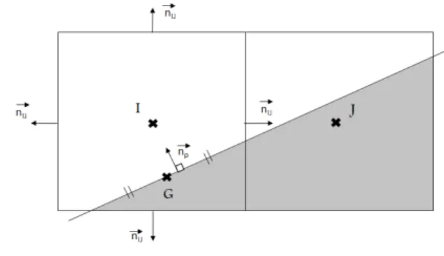
FIGURE 1: Sketch of cells crossed by the fluid-solid interface.

The previous sketch illustrates two cells I and J crossed by the interface (solid being grey, fluid white). Here, the porosity and the volumetric fractions are known in each cell. Conse-quently, it is possible to determine the face fraction between I and J.

Interface center of gravity per cell In order to de-fine the pressure gradient in the cells crossed by the interface, it is necessary to compute the interface center of gravity per cell. Consequently, in a finite volume formulation, for a cell I

crossed by the interface the fluid volume is defined like :

αIΩ =

_∑

J

αIJ~xGIJ.~nIJ+~xGP.~nP (11)

with Ω the total cell volume, αI the cell volumetric fraction,

αIJthe face volumetric fraction, xGthe face center of gravity,

and ~nPthe normal vector of the interface considered as a fifth

face in this kind of cell. For each cell, the normal vectors are defined by :

∑

J

αIJ~nIJ+~np= 0 (12)

The interface center of gravity is then extracted from these two equations. Fig.1 illustrates the different points and surface vec-tors.

Pressure gradient re-construction at the interface

When a cell is crossed by the interface as in Fig.1, the pressure at the fifth face is approached with :

PFSI= PI+ ~IGP. ~∇P (13)

In finite volume, the pressure gradient is for the cell I :

Z

Ωi

∇Pdx =

_∑

J

αIJPIJ+ PFSI~np (14)

Thanks to the previous relation on normal vectors, the pressure gradient comes with:

αI∇PΩ =~

∑

J

αIJ(PIJ− PI)~nIJ+

∑

J

αIJ( ~IGP. ~∇P)~nIJ (15)

VIBRATING CYLINDER IN A FLUID

First, the interface treatment is illustrated for the TSDP method. Then, in order to assess the quality of each fixed do-main interface tracking method, a comparison is achieved on a vibrating square cylinder in a fluid at rest. The ALE method from Code_Saturne is considered in this case as the analitical solution. The TSDP method is compared to ALE for a high amplitude vibrating cylinder in a fluid at rest and tested in a cross flow.

Highlights on the interface treatments with the mov-ing porosity.

On Fig. 2, it is possible to see that the solid is meshed, the porosity defines the solid. Where the porosity is 0, the domain is penalized, the velocity is the solid one. For each cell crossed by the interface, the fluid characteristics are required for the neighboring cells. Consequently, even if the volume of fluid is smaller than the solid one, velocity and pressure are computed to ensure the continuity. The velocity field and the pressure for each cell is illustrated in the case of a cylinder moving down in Fig. 2.

FIGURE 2: Fluid-solid interface treatment example.

Vibration of a cylinder in a fluid at rest.

In the present work, the square cylinder diameter is Dc= 4

cmand 40 cm, and for the domain Dd= 120 cm therefore it

is an infinite domain. The cylinder is vibrating according to

Vs(t) = D₂₀cω sin(ωt)~eyand Vs(t) = D₁₀cω sin(ωt)~eywith ω = 10

rad/s. The mesh is the same for the three different methods.

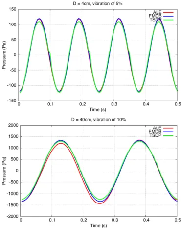
FIGURE 3: Comparison of the three methods for a square D = 4cm and D = 40cm vibrating with an amplitude of 5% and 10% of its diameter.

On Fig. 3, the pressure is presented as a function of time for a fixed point above the square with the three fluid-solid interface tracking methods. For a vibration of 5% and 10% of the square diameter, FMDE and ALE formulations are in agreement. In fact, the Taylor development is more accurate within this range of vibration. The TSDP gives the same period with a slight difference in amplitude. Results are consequently encouraging given that the pressure profile is well defined for fixed grid postulations.

Now, it is necessary to complete the study, with large am-plitude of vibration. In this configuration, the transpiration method is not consistent because of Taylor’s expansion limi-tation. To be able to simulate the fluidelastic instability, the method has to be robust enough to deal with large amplitudes of vibration. A cylinder with a diameter of 20 cm in water at rest is defined. The domain is a square with a side of 1.2 m. In order to show the stability of the method, a vibration of 25% of the diameter is computed, the results for pressure and velocity at a point above the cylinder are the following :

FIGURE 4: Pressure profile above a cylinder (D = 20cm) vi-brating with an amplitude of 25% of its diameter.

The monitoring point is still above the cylinder which explain for such high amplitude the pressure profile. Moreover, the signal periodicity shows the quality of the representation

from both methods. Here, the ALE is considered as the

reference in our study. It is possible to see that there is a reasonable agreement between both methods. However, they are slightly different, but results are encouranging.

This short study done as a feasibility assessment, shows the potential of moving porosity on fixed grid.

Imposed vibration of a cylinder in a cross-flow with the TSDP method.

In order to show the future possibilities of the method, the

same simulation is achieved with a cross-flow : ~u = 1 ~exm/s,

the movement of the cylinder is still imposed. There is no tur-bulent model, this study aims at showing the good behaviour of the method and its numerical stability.

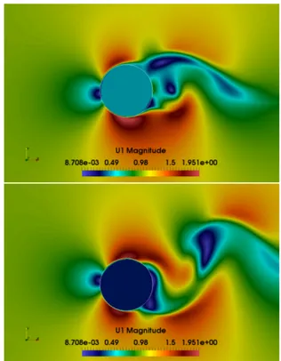
FIGURE 5: Velocity field around a vibrating cylinder with the TSDP method at t = 0.75, and 1.00 s.

On Fig. 5, the velocity field around the vibrating cylinder is represented at different times (0.75 and 1.00 s). The impact of the vibration on the velocity field is reasonably reproduced by the acceleration at the top for a cylinder going up, and at

the bottom for a cylinder going down. Moreover, pictures

illustrate the capabilities to follow the fluid-structure interface

thanks to porosity. The solid velocity is also represented

inside the cylinder as it is meshed. This feasibility test gives

us the possibilities of this kind of method. The different

novelties we proposed, have to be improved to deal with the different existing types of mesh, with turbulent models, with several cylinders and mainly to deal with two-phase flows. Consequetly, according to the encouraging results of the primary developments, the study will be continued to evaluate its agreement with the physical properties of this kind of case (Stokes number, Strouhal number, phase lag...).

LIQUID-VAPOR FLOW IN AN INCLINED CYLINDER ARRAY

For this study, prediction of void fraction, and gas veloc-ity are compared to experimental data in order to determine the most fitted model for two-phase flow in cylinder array, this ex-periment was performed by CEA and called MAXI2 [25, 26].

Experiment

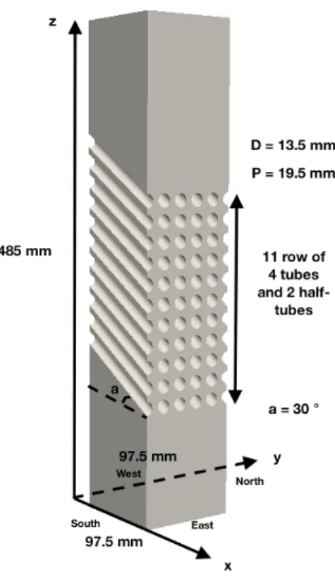
The experimental device is a square channel with 11 rows of 5 inclined cylinders (4 tubes and 2 half-tubes) with an angle

a= 30. The geometry is illustrated in Fig. 6.

FIGURE 6: Sketch of the cylinder array.

The experiment involves a saturated freon (R114) liquid-vapor flow. The physical properties are respectively for liquid and vapor:

Volumetric mass (kg/m3_{): ρ}

l= 1273, 974, ρg= 63, 166;

Viscosity (Pa.s): µl= 2, 066.10−4, µg= 1, 382.10−5;

Surface tension (N/m): σ = 6, 005.10−3;

Temperature and pressure (K and Pa): Tre f = 350.40,

Pre f = 8, 7.105.

Initially, there is only liquid in the channel. At the inlet, the liquid and gas velocities are 0.183 m/s and 0.319 m/s with

22% of void fraction. At the outlet, the pressure is 8, 7.105Pa.

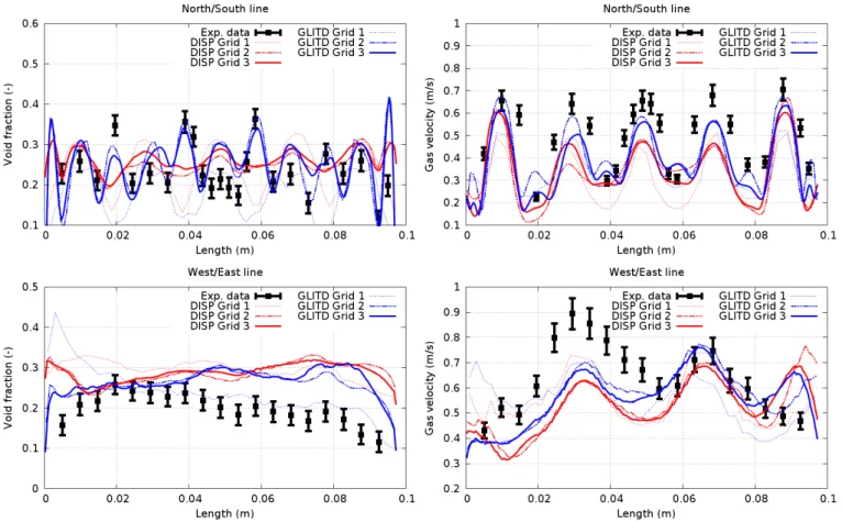
Void fraction and gas velocity are measured along the line North − South (NS) defined by x = 48.75mm and z = 276.36mm, and the line West − East (WE) defined by y = 48.75mm and z = 276.36mm.

For this study, prediction of void fraction, and gas velocity are compared to experimental data in order to determine the most fitted model for two-phase flow in cylinder array.

Results with the dispersed and the generalized ap-proach

The results are presented with three mesh refinements of 0.7, 7 and 70 millions of fully hexahedra cells. The

predic-tions of void fraction and gas velocity along the two lines of measurement are computed with the dispersed (DISP) and dis-persed to large interface flow (GLITD) models.

Void fraction predictions First, it is important to highlight that the results are time-averaged. The left side of Fig. 7 presents time-averaged void fraction simulation results using the two different models and compared to experimental data along the lines North-South and East-West.

On one hand, based on the dispersed bubbly flow ap-proach, the simulation is roughly matching the experimental data. In front of the cylinders, the prediction is less accurate than between (in the “axial flow”). In fact, the averaged void fraction tendency is not even captured in front of cylinders. At walls, the impact of the wall force seems to be not negligible because of the over-estimations.

On the other hand, based on the generalized large interface to dispersed bubbly flow approach, the tendency of the aver-aged void fraction is well captured even in front of cylinders.

FIGURE 8: Instantaneous void fraction contours of 30% (left) and 36% (right), DISP approach.

Fig. 8 and Fig. 9 represent void fraction contours with each model (30% and 36% for DISP model and 50% for GLITD model).On Fig. 8, what we can see is that the DISP model does not predict instantaneous void fractions higher than 36%. In comparison, on Fig. 9, the GLITD model can predict higher void fractions at an instant t, the fluctuations are more impor-tant with this model. However, averaged void fractions from both models lead approximately to the same results.

In this configuration, the range of void fraction is large, other studies should be performed for different higher and lower void fractions in further calculations.

Gas velocity predictions The right side of Fig. 7 presents time-averaged gas velocity simulation results using the two different models and compared to experimental data along the lines North-South and East-West. The averaged gas velocity of both models is closer to the experimental data than the averaged void fraction prediction. The tendency is well

FIGURE 7: Results for void fraction and gas velocity along NS and WE with both two-phase flow models.

FIGURE 9: 50% instantaneous void fraction contour, GLITD approach.

captured by both models, but the generalized large interface to dispersed bubbly flow seems to be closer to the experimental data.

CONCLUSION

In order to determine the different methods required for modeling vibration induced by two-phase flow, three fluid-structure interface tracking methods and two two-phase flow models are compared separately.

Based on a penalization method and a porosity depend-ing on the cell location (fluid or solid), the interface track-ing method, called “Time and Space Dependent Porosity”, is in good agreement with the analytical solution with a reduced computation time in comparison with ALE. The limitation of the FMDB method is due to its Taylor expansion highlighted by increasing the vibration amplitude. Three methods are in agreement for slight vibrations under 10% of their diameter, then for high amplitude of vibration the TSDP gives encourag-ing results in comparison with ALE.

The dispersed bubbly and generalized large interface to dispersed bubbly flow approach have been compared on a two-phase cross-flow in an inclined cylinder array described previ-ously. The study carried out for three mesh refinements shows the deficiency of the dispersed bubbly approach for high void fractions. However, the second method taking avantage from dispersed bubbly and large interface model gives promising

results and correct agreement with experimental data. The

present work is still in progress, both models have to be tested on different cylinder array, and for different range of void frac-tion. The next step will be to compare the fluid forces around static and moving cylinders with the chosen approach.

ACKNOWLEDGMENT

Authors want to thank both EDF R&D projects: Qual-IFS-GV, devoted to the assessment of SG tube vibration risk; and NEPTUNE funded by EDF (Electricité de France), CEA (Commissariat à l’Energie Atomique et aux Energies Alterna-tives), AREVA-NP and IRSN (Institut de Radioprotection et de Sureté Nucléaire).

REFERENCES

[1] A. Guelfi, D. Bestion, M. Boucker, P. Boudier, P. Fil-lion, M. Grandotto, J.-M. Hérard, E. Hervieu, P.Peturaud., NEPTUNE - A New Software Platform for Advanced Nuclear Thermal-Hydraulics, Nuclear Science and Engi-neering, 2007.

[2] S. Mimouni, F. Archambeau, M. Boucker, J. Laviéville, C. Morel, A second order turbulence model based on a Reynolds stress approach for two-phase boiling flow. Part 1: Application to the ASU annular channel case, Nuclear Engineering and Design, 2009.

[3] S. Mimouni, F. Archambeau, M. Boucker, J. Laviéville, C. Morel, A second order turbulence model based on a Reynolds stress approach for two-phase boiling flow. Part 1: Adiabatic cases, Technology of Nuclear Installations, 792395, 2009.

[4] S. Mimouni, F. Archambeau, M. Boucker, J. Laviéville, C. Morel, A second order turbulence model based on a Reynolds stress approach for two-phase boiling flow and application to fuel assembly analysis, Nuclear Engineer-ing and Design, 2010.

[5] S. Mimouni, J. Laviéville, N. Seiler, P. Ruyer, Combined evaluation of second order turbulence model and polydis-persion model for two-phase boiling flow and application to fuel assembly analysis, Nuclear Engineering and De-sign, 2011.

[6] C. Morel, P. Ruyer, N. Seiler, J. Laviéville, Comparison of several models for multi-size bubbly flows on an adi-abatic experiment, International Journal of Multiphase Flow, 2010.

[7] M. Ishii, N. Zuber, Drag coefficient and relative velocity in bubbly, droplet or particulate flows, American Institute Chemical Engineers Journal, 1979.

[8] P. Ruyer, N. Seiler, M. Beyer, F.P. Weiss, A bubble size distribution model for the numerical simulation of bub-bly flows, International Conference on Multiphase Flow, 2007.

[9] A. Tomiyama, H. Tamai,I. Zun, S. Hosokawa, Transverse migration of single bubbles in simple shear flows, Chem-ical Engineering Science, 2002.

[10] N. Zuber, On the dispersed two-phases flow in the laminar flow regime. Chemical Engineering Science, 1964. [11] E. Krepper, B. Koncar, Y. Egorov, CFD modeling of

sub-cooled boiling – concept, validation and application to fuel assembly design, Nuclear Engineering and Design, 2007.

[12] P. Coste, A Large Interface Model for two-phase CFD, Nuclear Engineering and Design, 2013.

[13] J. Laviéville, P. Coste, Numerical modeling of liquid-gas

stratified flows using two-phase Eulerian approach, Inter-national Symposium on Finite Volumes for Complex Ap-plications, 2008.

[14] P. Coste, J. Pouvreau, C. Morel, J. Laviéville, M. Boucker, A. Martin, Modeling turbulence and friction around a large interface in a three-dimension two-velocity eulerian code, NURETH-12, 2007.

[15] P. Coste, J. Pouvreau, J. Laviéville, M. Boucker, A two-phase CFD approach to the PTS problem evaluated on COSI experiment, ICONE, 2008.

[16] P. Coste , J. Laviéville, A Wall Function-Like Approach for-Two-Phase CFD Condensation Modeling of the Pres-surized Thermal Shock, NURETH-13, 2009.

[17] N. Merigoux, J. Laviéville, S. Mimouni, M. Guingo, C. Baudry, A generalized large interface to dispersed bubbly flow approach to model two-phase flows in nuclear power plant, CFD4NRS-6, 2016.

[18] F. Huvelin, Couplage de codes en interaction fluide-structure et applications aux instabilités fluide-élastiques, Thèse de doctorat, Ecole doctorale des Sciences Pour l’Ingénieur de Lille, 2008.

[19] E. Deri, J. Nibas, O. Ries, A. Adobes, Measurement of flow-induced forces: a single flexible tube in a rigid triangular-pitch bundle subjected to two-phase cross-flow, Pressure Vessels & Piping, 2015.

[20] V. Shinde, E. Longatte, F. Baj, Large Eddy Simulation of fluid-elastic instability in square normal cylinder array, Pressure Vessels & Piping, 2015.

[21] Y. Jus, E. Longatte, J.C. Chassaing, P. Sagaut, Low-mass damping vortex-induced vibrations of a single cylinder at moderate Reynolds number, Journal of Pressure Vessel Technology, 2014.

[22] M.V Girao de Morais, Qualification numérique des méthodes de modélisation des forces fluide-élastiques s’exerçant dans un faisceau de tubes en écoulement transversal, Thèse de doctorat, Université d’Evry Val d’Essonne, 2006.

[23] M.Á. Fernandez-Varela, Modèles simplifiés d’interaction fluide-structure, Thèse de doctorat, Université Paris IX Dauphine, 2001.

[24] A. Doradoux, Développement d’une méthode de cou-plage fluide-structue en diphasique avec présence d’un gaz condensable ,Thèse de doctorat, Université de Bor-deaux, 2016.Ph.D still in progress.

[25] C. Bouillet, M. Grandotto, S .Pascal, Comparison be-tween a simulation and local measurements of a two-phase flow across a 60 inclined tube bundle, International Congress on Multiphase-Flows, 2007.

[26] D. Soussan, A. Gontier, V. Saldo, Local two-phase flow measurement in an oblique tube bundle geometry - the MAXI program, International Congress on Multiphase-Flows, 2001.

View publication stats View publication stats