HAL Id: hal-00105949
https://hal.archives-ouvertes.fr/hal-00105949
Submitted on 7 Dec 2016
HAL is a multi-disciplinary open access
archive for the deposit and dissemination of
sci-entific research documents, whether they are
pub-lished or not. The documents may come from
teaching and research institutions in France or
abroad, or from public or private research centers.
L’archive ouverte pluridisciplinaire HAL, est
destinée au dépôt et à la diffusion de documents
scientifiques de niveau recherche, publiés ou non,
émanant des établissements d’enseignement et de
recherche français ou étrangers, des laboratoires
publics ou privés.
Ocean: A closer look at lithospheric cooling
Alessia Maggi, Eric Debayle, Keith Priestley, Guilhem Barruol
To cite this version:
Alessia Maggi, Eric Debayle, Keith Priestley, Guilhem Barruol. Multi-mode surface waveform
tomog-raphy of the Pacific Ocean: A closer look at lithospheric cooling. Geophysical Journal International,
Oxford University Press (OUP), 2006, 166 (3), pp.1384-1397. �10.1111/j.1365-246X.2006.03037.x�.
�hal-00105949�
GJI
T
ectonics
and
geo
dynamics
Multimode surface waveform tomography of the Pacific Ocean: a
closer look at the lithospheric cooling signature
Alessia Maggi,
1Eric Debayle,
1Keith Priestley
2and Guilhem Barruol
3,∗1CNRS and Universit´e Louis Pasteur, 67084 Strasbourg, France. E-mail: [email protected] 2Bullard Laboratories, University of Cambridge, Cambridge, CB3 0EZ, UK
3Laboratoire de Tectophysique, CNRS, Universit´e Montpellier II, Montpellier, France
Accepted 2006 April 6. Received 2006 March 16; in original form 2005 September 9
S U M M A R Y
We present a regional surface waveform tomography of the Pacific upper mantle, obtained using an automated multimode surface waveform inversion technique on fundamental and higher mode Rayleigh waves, to constrain the VSV structure down to∼400 km depth. We have improved on previous implementations of this technique by robustly accounting for the effects of uncertainties in earthquake source parameters in the tomographic inversion. We have furthermore improved path coverage in the South Pacific region by including Rayleigh wave observations from the French Polynesian Pacific Lithosphere and Upper Mantle Experiment deployment. This improvement has led to imaging of vertical low-velocity structures associated with hotspots within the South Pacific Super-Swell region. We have produced an age-dependent average cross-section for the Pacific Ocean lithosphere and found that the increase in VSVwith age is broadly compatible with a half-space cooling model of oceanic lithosphere formation. We cannot confirm evidence for a Pacific-wide reheating event. Our synthetic tests show that detailed interpretation of average VSV trends across the Pacific Ocean may be misleading unless lateral resolution and amplitude recovery are uniform across the region, a condition that is difficult to achieve in such a large oceanic basin with current seismic stations.
Key words: lithosphere, Pacific Ocean, plate tectonics, Rayleigh waves, tomography.
1 I N T R O D U C T I O N
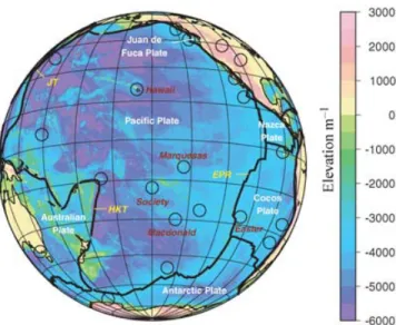
The Pacific region (Fig. 1) is a natural laboratory for oceanic plate tectonics. It is the home of the oldest contiguous oceanic plate from mid-ocean ridge to subduction (Pacific Plate, 0–170 Ma), as well to four other exclusively oceanic plates (Juan de Fuca, Philippine, Cocos and Nazca). It is bounded on three sides by subduction zones, and contains four distinct mid-ocean ridges (East Pacific Rise, Gala-pagos Rise, Chile Rise and Pacific–Antarctic ridge). More detailed images of these structures, and of the expanses of plates between them, are necessary if we wish to improve our understanding of the structure and evolution of oceanicplates.
The upper mantle structure of the Pacific Ocean, where we ex-pect to see the signature of plate tectonics, is best investigated us-ing seismic surface waves. The majority of studies that cover the whole Pacific Ocean use measurements of fundamental mode Love and/or Rayleigh dispersion to constrain the uppermost 300 km of the mantle, either alone (Nishimura & Forsyth 1988, 1989; Montagner
∗Also at: Lab. Terre Oc´ean, Univerist´e de Polyn´esie fran¸caise, Tahiti, French
Polynesia.
& Tanimoto 1991; Ekstr¨om et al. 1997; Boschi & Ekstr¨om 2002; Montagner 2002; Ritzwoller et al. 2002; Trampert & Woodhouse 2003; Beghein & Trampert 2004; Ritzwoller et al. 2004; Levshin
et al. 2005), or in a joint inversion with body wave phases and
nor-mal modes which provide a better constraint on the lower mantle (Ekstr¨om & Dziewonski 1998; Beghein et al. 2002) . A few studies improve the resolution of the base of the upper mantle by includ-ing observations of higher mode surface waves, either explicitly (Van Heijst & Woodhouse 1999; Ritsema et al. 2004) or as part of a waveform inversion procedure (M´egnin & Romanowicz 2000; Gung et al. 2003).
Surface wave studies of the Pacific Ocean upper mantle are ham-pered by the geographical distribution of seismic stations, which being almost exclusively land based are concentrated at the borders of the region. As the vast majority of earthquakes are also concen-trated along the subduction zones that form the Pacific Rim, surface wave coverage of the expanse of the Pacific Ocean can only be ob-tained by using very long propagation paths (10 000–15 000 km). The lateral extent of the sensitivity zone for surface waves increases with path length (Spetzler & Snieder 2001; Yoshizawa & Kennett 2002), therefore, even with good path density and azimuthal cover-age the use of long propagation paths effectively limits the lateral resolution of surface wave tomographic images to∼1500 km, too
Figure 1. Outline map for the Pacific Ocean region, showing location of major features mentioned in the text. Topography and bathymetry are from SRTM30. Hotspots according to Courtillot et al. (2003) are shown as open circles and plate boundaries are drawn as thick black lines. Labelled hotspots and plate boundaries are mentioned explicitly in the text. Abbreviations are: HKT—Hikurangi–Kermadek–Tonga, JT—Japan Trench and EPR— East Pacific Rise.
wide to provide meaningful images of narrow features such as mid-ocean ridges, subduction zones and hotspots.
This present study was prompted by the installation in 2001 of ten broadband stations in French Polynesia as part of the Pacific Lithosphere and Upper Mantle Experiment (PLUME) described by Barruol et al. (2002). These stations provided us with addi-tional path coverage in the normally under-sampled South Pacific, allowing us to improve our lateral resolution compared to previ-ous studies. We used a two-stage waveform tomography method that combines the automated multimode surface waveform in-version of Debayle (1999) with the highly efficient Debayle & Sambridge (2004) tomographic algorithm and is described in Sec-tion 2. This procedure increases our sensitivity to the upper man-tle shear wave velocity structure below∼300 km depth compared to studies that use only fundamental mode surface waves. We have improved on previous implementations of this method (e.g Debayle et al. 2001; Priestley & Debayle 2003; Sieminski et al. 2003; Pilidou et al. 2004) by explicitly and robustly accounting for the effects of uncertainties in earthquake source parameters as described in Section 2.3.
Our resulting tomographic model, presented in Section 3, pro-vides images of the Pacific upper mantle shear wave velocity structure with varying horizontal resolution. The best resolution is obtained in the subduction zone regions, where our images of subducted slabs are comparable with regional body wave studies (Gorbatov & Kennett 2003) and surface wave studies of smaller re-gions (Lebedev & Nolet 2003). In the region known as the South Pacific Super-Swell, we find low shear wave velocity anomalies that are confined to localized structures associated with several major hotspots of the region. Our tomographic results contain a strong age-dependent signature within the oceanic lithosphere, which we discuss in detail in Sections 3.1 and 4, comparing average
VSV-age profiles with predictions from standard half-space cooling
and plate cooling models, and with a recent observation by
Ritz-woller et al. (2004) of a punctuated thermal history in the Pacific Ocean.
2 D AT A A N D M E T H O D S
We have analysed vertical component Rayleigh wave seismograms from all earthquakes of magnitude greater than MW5.5 that occurred
between 1977 January and 2003 April, and for which the R1 portion of the surface waves propagated exclusively in the Pacific Ocean hemisphere (i.e. between 120E and 300E). These earthquakes oc-curred mostly on the subduction zones surrounding the Pacific Plate, and to a lesser extent on the mid-ocean ridges. The vast majority of our recordings were obtained from the public IRIS (Incorporated Research Institutions for Seismology) database, with the addition of a few thousand recordings from 2 yr of temporary deployment of 10 seismograph stations in French Polynesia (PLUME, Barruol et al. 2002). These Polynesian records provide extra coverage in the South Pacific, allowing us to improve the resolution in this region com-pared to previous studies. Our full data set contains several hundred thousand seismograms.
Our surface waveform tomography is based on a two-stage proce-dure that has proved to be successful in a number of recent regional-scale studies (e.g. Debayle et al. 2001; Priestley & Debayle 2003; Sieminski et al. 2003; Pilidou et al. 2004). We have modified the procedure used in these previous studies to ensure a smooth data cov-erage and to account for the uncertainties introduced by errors in earthquake focal parameters. In the following two sections, we give a brief overview of the two-stage waveform tomography method. A more detailed description of our improvement to this method is given in Section 2.3.
2.1 Surface waveform inversion
In the first stage of the tomographic process, we model vertical com-ponent long period (50–160 s) Rayleigh wave seismograms to obtain path-averaged values of the upper mantle shear wave velocity along great-circle paths between earthquakes and seismograph stations. We use the method of secondary observables originally proposed by Cara & L´evˆeque (1987), and later automated by Debayle (1999), to reduce the non-linearity of the waveform inversion. Rayleigh waves are primarily sensitive to the propagation speed of vertically polarized shear waves, VSV. The mantle part of our starting seismic
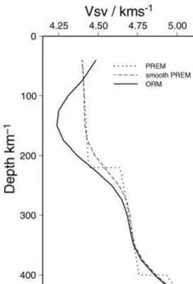
velocity model for each path is the smoothed version of the 1-D VSV
profile from PREM (Dziewonski & Anderson 1981) shown in Fig. 2. The crustal portion is not inverted for, and is adapted to each path by averaging the crustal part of the 3SMAC (Nataf & Ricard 1995) 3-D model along the great circle path. Using a different 3-D crustal model (e.g. CRUST2.0, Mooney et al. 1998; Bassin et al. 2000), does not change our waveform modelling results (see discussion in Pilidou et al. 2004). We model the fundamental mode Rayleigh wave together with its first four overtones, thereby increasing our sensitivity to the shear wave velocity structure at the base of the oceanic asthenosphere (∼300–400 km depth) compared to global and whole-Pacific studies that use only fundamental mode surface waves (Nishimura & Forsyth 1988, 1989; Montagner & Tanimoto 1991; Ekstr¨om et al. 1997; Boschi & Ekstr¨om 2002; Montagner 2002; Beghein & Trampert 2004; Ritzwoller et al. 2004; Smith
et al. 2004).
The automated multimode surface waveform inversion of Debayle (1999) imposes stringent data quality requirements, and rejects paths for which the waveform inversion does not converge.
Figure 2. 1-D reference models: the VSVprofile from PREM (dotted line,
Dziewonski & Anderson 1981); the mantle VSVstarting model for 1-D
in-version of Rayleigh waves (dashed line), derived from PREM using a cubic spline function; the Oceanic Reference Model (ORM) derived by averag-ing our tomographic results for oceanic regions between the ages of 30 and 70 Ma (solid line).
Only 56 217 waveforms out of the full data set described above met all of the requirements of the waveform inversion, and were in-cluded in our tomographic inversion. Fig. 3 shows the path density (number of paths per unit area) for these accepted waveforms, and illustrates the exceptional size of our data set. The path-averaged models from this study form half of the data set of the Debayle et al. (2005) global model.
Figure 3. (a) Geographical distribution of the events (filled circles) and stations (white diamonds) used in this study. Stations corresponding to the PLUME
experiment are shown as larger red diamonds. (b) Ray density for the 56 217 waveforms included in the tomography. The unit area is the area of a 1× 1◦cell
at the equator. The colour scale is saturated at 100 ray paths per unit area, however the path density exceeds 3000 ray paths per unit area in places, notably in the southwest Pacific.
2.2 Tomographic inversion of path-averaged models
In the second stage of the tomographic process, we combine the path-averaged upper mantle models from all the earthquake-station paths into a single tomographic inversion to obtain a 3-D model of shear wave velocity in the upper mantle. We use the Debayle & Sambridge (2004) tomographic algorithm, which has been optimized for the inversion of extremely large data sets. This algorithm is based on the continuous formulation of the inverse problem introduced by Montagner (1986); it simultaneously inverts for the isotropic and azimuthally anisotropic components of VSVusing a procedure
orig-inally described by L´evˆeque et al. (1998). Neighbouring points in the tomographic model are correlated using a Gaussian a priori covariance function that has been found to act as a crude but ef-fective sensitivity kernel by Sieminski et al. (2004). The lateral degree of smoothing in the 3-D model is controlled by the half-width of the Gaussian covariance function, also referred to as the correlation length Lcorr, while the amplitude of the perturbations
in the inverted model is controlled by an a priori model variance,
σM.
Our tomographic model is discretized on a 1◦× 1◦regular grid, us-ing a correlation length Lcorrof 400 km, and a priori model variances σMof 0.05 km s−1and 0.005 km s−1for the isotropic and anisotropic
components of the shear wave velocity, respectively. Increasing (de-creasing) Lcorr leads to smoother (rougher) tomographic images
with higher (lower) amplitude anomalies, but the overall pattern of anomalies remains unchanged. Increasing (decreasing)σMleads
to higher (lower) amplitude anomalies, but still leaves the overall pattern of anomalies unchanged. In this paper we discuss only the isotropic part of the model; the anisotropic part is discussed in detail in Maggi et al. (2006).
2.3 Path clustering and estimation of data errors
Most tomographic algorithms take into account the estimated uncer-tainty in the data (in our case the path-averaged shear wave velocity models) used to drive the inversion. In the following, we shall denote such uncertainties asσD to contrast them with the a priori model
approach, which both the Debayle & Sambridge (2004) inversion and its predecessor by Montagner (1986) are based upon, these data errors not only regulate the relative weight given to each datum within the inversion, but also regulate how far beyond the a priori model varianceσMthe inversion will push the final model in order
to fit the data within their errors.
However, if the data are unreliable and the data errors underesti-mate the true uncertainties, this same behaviour can lead to artefacts in the final result. Maggi & Priestley (2005) have shown that errors in earthquake epicentre, origin time and hypocentral depth directly affect the shear wave velocity models obtained by waveform inver-sion without any influence on the quality of the waveform fit. These source errors lead to erroneous path-averaged shear wave velocity models coupled with underestimated uncertainties, and cause arte-facts in the tomographic inversion. In order to reduce these artearte-facts, excessive smoothing is often used, leading to loss of horizontal res-olution and a decrease in data fit.
We can obtain a better estimate of the true path-averaged struc-ture by comparing multiple path-averaged measurements along re-peatedly sampled propagation paths. We cluster our path-averaged models geographically with a cluster radius of 200 km, and treat the shear wave models that form each cluster as independent mea-surements of the average shear wave velocity profileVS(z) along the
common path. We form our clusters by grouping all paths whose start and end points are within 200 km of the extremities of a cen-tral path chosen at random from the data set, while imposing that no path can belong to more than one cluster. The path-averaged profile,VS(z), and depth-dependent measurement error,σD(z),
as-sociated with each cluster are, respectively, the mean and the stan-dard deviation on the mean,σm(z) = σ(z)/
√
n, of the 1-D shear
wave velocity models of its n component paths. This choice ofσ
m gives more weight to better-sampled paths. Very small values
of σm(z) are commonly indicative of a path for which the data
has little resolution at depth z, and for which most of the 1-D shear wave velocity models have not moved away from the a priori value. Therefore, if for a cluster the value ofσm(z) at a
particu-lar depth is smaller than the average a posterior waveform fitting error of its component paths, then we use this average waveform fitting error instead ofσm(z) as an estimate of the data uncertainty σD(z).
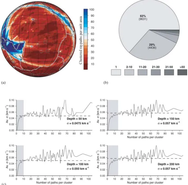
Clustering with a 200 km radius reduced the number of inde-pendent path-averaged shear wave velocity measurements in our data set from 56 217 to 15 165. The resulting path density, plot-ted in Fig. 4(a), is much smoother than that of the original data set shown in Fig. 3(b). Previously over-sampled regions such as Indone-sia, the westernmost Pacific, North America and certain corridors towards Hawaii and other ocean island stations now have compa-rable path density to the central and South Pacific regions, whose path density has not been significantly modified by the clustering procedure.
Of the 15 165 clustered ray paths, 63 per cent contain only one path (see Fig. 4b) and, therefore, represent a single shear wave ve-locity measurement with no error estimate other than the a posterior waveform fitting error. In order to use these single-path models in the tomography they need to be assigned a reasonable data error
σD. We have averaged at each depth all the standard deviations
cal-culated for a given cluster size n. We have found that this average standard deviation ¯σ(n)|z increases rapidly with cluster size n for
small clusters, before tending towards a constant value (see Fig. 4c). This suggests that the low value ofσ for the smaller clusters is simply a low-number sampling effect, and that if we had more data for these clusters, the standard deviation would increase to become
compat-ible with the larger clusters. We, use the flat portion of the ¯σ(n)|z
curve to set an equivalent ¯σ for small clusters, as shown in Fig. 4c, from which we calculate the correspondingσD(z)= ¯σ (n)|z/
√
n.
2.4 Horizontal resolution
Under the assumptions of ray theory, used throughout this study, sur-face waves cannot resolve structures smaller than the width of their sensitivity zone, estimates of which vary (e.g. Spetzler & Snieder 2001; Yoshizawa & Kennett 2002), but increase with surface wave period (increasing wavelength) and also with increasing path length. For example, according to Spetzler & Snieder (2001) the width of the sensitivity zone for a fundamental mode Rayleigh wave of 100 s period (the dominant period in our data set) increases from 1200 km for a 5000 km path to 1800 km for a 15 000 km path, while Yoshizawa & Kennett (2002) estimate the sensitivity zone to in-crease in width from 450 to 700 km, respectively. It is clear in both cases that in order to optimize our horizontal resolution, we have to maximize the proportion of short propagation paths in our data set. The distribution of path lengths in our data set is shown in Fig. 5(a). Approximately 75 per cent of our paths are shorter than 6000 km and, therefore, have lateral sensitivity zones between 450 and 1200 km wide according to Yoshizawa & Kennett (2002) and Spetzler & Snieder (2001), respectively. We have chosen to apply a correlation length Lcorrof 400 km to the tomographic
in-version, corresponding to a Gaussian sensitivity zone around each path with a width of 800 km, which is in the centre of the range of sensitivity zone estimates for 100 s fundamental mode Rayleigh waves.
For large data sets such as that presented in this study, the width of the surface wave sensitivity zone physically degrades the hor-izontal resolution from the geometrical resolution determined by the path coverage alone. Fig. 5(b) shows a representation of the geometrical resolution limit of our clustered path coverage as an optimized Voronoi diagram in the style of Debayle & Sambridge (2004). In order to correctly retrieve both isotropic and azimuthally anisotropic components of VSV in a given region, we need to
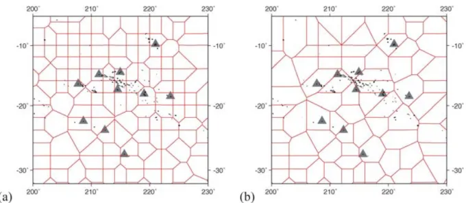
re-solve the 2θ Rayleigh wave periodicity caused by an azimuthally anisotropic medium. This requires at least three paths crossing the region with sufficiently different azimuths. The Voronoi diagram in Fig. 5(a) illustrates the size of the regions for which our data set satis-fies this geometrical criterion. The size of the Voronoi cells increases from a starting size of 2◦in the western and southeastern Pacific, towards cells of width up to 10◦–15◦in the central Pacific, indicat-ing that lateral resolution determined by the path coverage varies from better than 200 km in the best-sampled regions to∼1500 km in the more sparsely sampled central Pacific. The relatively small Voronoi cells in the South Pacific region are due to the additional data provided by the PLUME deployment which provide 141 out of 680 clustered paths in the region, as illustrated in Fig. 6. The geometrical lateral resolution described by the Voronoi diagrams is further degraded by the correlation length imposed on the inver-sion, which reflects the finite width of the surface wave sensitivity zone as described above. We estimate the actual horizontal reso-lution to be∼600 km in the northwestern Pacific, which has both the densest path coverage and the largest proportion of short paths, and∼800 km in the South Pacific Super-Swell region. The Voronoi diagrams should be used in conjunction with the path density plot of Fig. 4(a) when interpreting the tomographic results in the following section.
Figure 4. (a) Ray density for the 15 165 clusters. The unit area is the same as for Fig. 3. (b) The distribution of cluster sizes. Shading indicates the range of cluster sizes (1 path, 2–10 paths, 11–20 paths etc.); the percentage of clusters that fall in the two most populated bins are shown on the pie-chart, above the
number of clusters in the bin (in brackets). (c) The averageσ for clusters vs. cluster size at depths of 50 to 200 km (solid lines). The average σ oscillates around
a central value ¯σ (z) indicated by the dashed lines and given within the plot. For each depth, the range of cluster sizes for which small number statistics seem to
apply (10–15) is highlighted in grey.
3 R E S U L T S
The results of our tomographic inversion are shown in Fig. 7, plotted as percentage deviations from the Oceanic Reference Model (ORM) of Fig. 2. ORM was derived by averaging our tomographic model for oceanic regions of age between 30 and 70 Ma and of ocean depth between 4500 and 5000 m (see Ritsema & Allen 2003), and is significantly slower than PREM above 300 km depth, confirming the observation by Ekstr¨om & Dziewonski (1998) that the Pacific upper mantle is unusually slow. Below 300 km depth, ORM ap-proaches the smoothed PREM model used as a starting model in our 1-D waveform inversion stage. We have inverted simultane-ously for both isotropic VSVand azimuthal anisotropy as discussed
above, though here we plot only the isotropic component of the
VSV distribution, as discussion of the azimuthally anisotropic
sig-nal is beyond the scope of this paper. This anisotropic sigsig-nal is
similar to that obtained for the Pacific region using our data by Debayle et al. (2005), and is described in detail in Maggi et al. (2006).
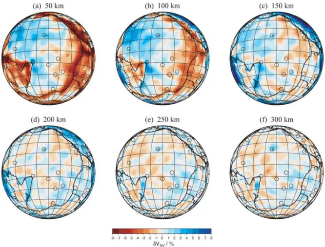
At shallow depth (50 km) the isotropic VSV distribution closely
reflects regional tectonics: mid-ocean ridges and back-arc regions are outlined by slow velocities, the subduction zones are outlined by faster velocities, and the velocities increase progressively across the Pacific plate from East to West as the lithospheric age increases. At this depth, the continents are slower than ORM. At 100 km depth the mid-ocean ridge signatures are less continuous, the increase in
VSVwith lithospheric age is still visible and the continental cratons
of Australia and North America now appear as strong high-velocity anomalies. At 150 km depth the ridge signatures have disappeared, while the subduction zones are clearly visible and the continental craton signatures are very strong. At 200 km depth the variation in
Figure 5. (a) Histogram of path lengths within the clustered data set. (b) Voronoi diagram in the style of Debayle & Sambridge (2004) for our clustered data set.
Figure 6. (a) Blow-up of the Voronoi diagram of Fig. 5(a) in the region of the South Pacific Super-Swell. The PLUME stations are indicated by grey triangles,
and contribute∼20 per cent of the paths crossing the region. (b) The Voronoi diagram with the paths contributed by the PLUME stations removed.
Tonga-Kermadec subduction zone and continental cratons, which are underlain by faster velocities until∼250 km depth.
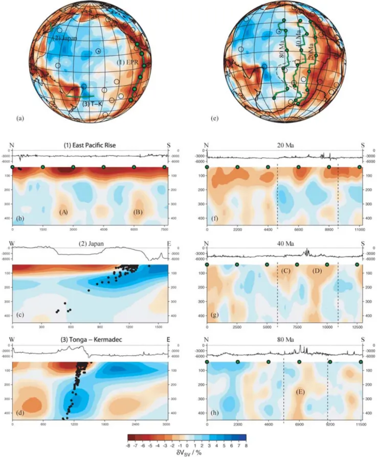
Fig. 8 shows selected cross-sections through our tomographic model. A cross-section running the length of the East Pacific Rise from north to south (Fig. 8b) shows longitudinal variations in the strength of the low-velocity anomaly corresponding to the oceanic ridge. It also suggests the presence of slower regions at depths be-tween∼300 and 400 km near the triple junction of the EPR and the slow-spreading Galapagos Rise (A), and near the Easter Island Hotspot (B). Cross-sections through two major subduction zone trenches, Japan, and Tonga–Kermadec, are shown in Figs 8(c)–(d). Our image of the Japan trench shows an∼150 km thick fast anomaly that descends into the mantle down to at least∼250 km depth, with seismicity outlining its upper surface. We can resolve this thin sub-ducting plate using surface waves thanks to an extremely dense
cov-erage of short-range paths in the region surrounding Japan. In our image, the slab is better defined than in the global model S20RTS (Ritsema et al. 1999). Our image is similar to that obtained in a smaller regional surface wave study of Southeast Asia by Lebedev & Nolet (2003), and to the upper 250 km of the image obtained by the Gorbatov & Kennett (2003) regional body wave study of the Western Pacific subduction zones, in which the Japan slab is seen to bottom out at transition zone depths. The Tonga-Kermadec trench shown in Fig. 8(d) also lies in a region of extremely dense coverage (see Fig. 4a), and is visible in our tomographic image well into the transition zone. A similar image of this slab is obtained by Gorbatov & Kennett (2003), also showing the slab penetrating the transition zone. The difference in our resolution of the subducting slabs below Japan and Tonga–Kermadec at depths>300 km is due to the dif-ferent illumination by higher mode surface waves, more prevalent
Figure 7. Horizontal slices through our tomographic model showing isotropic VSVat (a) 50 km, (b) 100 km, (c) 150 km, (d) 200 km, (e) 250 km and (f)
300 km depth. Throughout this paper, unless otherwise noted, tomographic results are plotted as a percentage variation with respect to the ORM model of Fig. 2. Azimuthal anisotropy results are not plotted on the tomographic slices for clarity, although anisotropy was taken into account in the inversion.
in the Tonga-Kermadec region thanks to the much larger number of deep focus earthquakes.
Panels (e)–(h) in Fig. 8 focus on our tomographic results for the South Pacific Super-Swell region, a shallow bathymetric anomaly (indicated by a dashed line in Fig. 8e) that has been postulated to be the surface expression of a large-scale mantle super-plume in the southcentral Pacific Ocean (see e.g. McNutt & Fischer 1987; Sichoix et al. 1998; M´egnin & Romanowicz 2000). This region is characterized by an increased rate of volcanism compared to other oceanic regions of similar age, and has been reported as having anomalously slow shear wave velocity by a number of surface wave tomographic studies (e.g. Ekstr¨om & Dziewonski 1998; Montagner 2002). Although a detailed discussion of the origin and implications of the anomalous bathymetry and volcanism are outside the scope of this paper, we would like to comment on the shear wave velocity structure of this region in the light of the improved coverage and hor-izontal resolution afforded to us by the PLUME data. In Fig. 8 panels (e)–(h) we show cross-sections through the Super-Swell region and the adjacent regions of the Pacific plate, taken along the 20, 40 and 80 Ma isochrons as defined by M¨uller et al. (1997). The 20 Ma pro-file shows a localized low shear wave velocity anomaly within the Super-Swell region confined to the upper 100–150 km of the mantle. The anomaly is underlain by a region with shear wave velocities up to 3 per cent faster than those in North Pacific plate mantle of the same age. The 40 Ma profile shows two low-velocity anomalies (C and D) within the Super-Swell region, associated with the approximate
locations of the Marquesas and Macdonald hotspots, respectively. The anomaly associated with the Macdonald hotspot (D) is contin-uous down to∼420 km depth, as is the broad low-velocity anomaly at the northern end of this profile, indicating a possible thermal upwelling from the transition zone. The 80 Ma profile shows a nar-row low-velocity anomaly (E), apparently also of thermal origin, rising from the transition zone close to the location of the Society hotspot. Furthermore, the northern portion of this profile shows a high-velocity anomaly associated with the approximate location of the Hawaiian hotspot. Detailed discussion of these hotspot related shear wave velocity anomalies, and interpretation of their thermal or chemical origin (e.g. Richardson et al. 2000; Tommasi et al. 2004), is outside the scope of this paper, and will not be engaged in here. It seems clear from Fig. 8, however, that the low-velocity anomalies in the Super-Swell region, imaged with higher resolu-tion thanks to the data from the PLUME experiment, are confined to localized structures, and are not pervasive throughout the entire area.
3.1 Shear wave velocity structure and oceanic age
The longest wavelength feature of the tomographic model shown in Fig. 7 is the increase in VSVwith increasing ocean age, progressing
from East to West across the Pacific plate. In Figs 9(a) and (b) we compare the shear wave velocity distribution at 100 km depth with the lithospheric ages given by M¨uller et al. (1997). The age
Figure 8. Selected cross-sections through our tomographic model. (a) Location of cross-sections shown in panels (b)–(d). (e) Location of cross-sections shown in panels (f) to (h); the approximate boundary of the region of anomalously elevated seafloor topography known as the South Pacific Super-Swell is indicated by a dashed line. The intersections of this boundary with the 20–80 Ma isochron profiles in panels (f)–(h) are indicated by vertical dashed lines. Green/black circles along the EPR profile in (a) and the 20–80 Ma isochron profiles in (e) correspond to the circles in panels (b), (f)–(h) and are used as distance markers. Seafloor topography profiles from Smith & Sandwell (1997) are shown above each tomographic cross-section. All tomographic images are plotted as percentage variation with respect to the 1-D ORM model of Fig. 2. Earthquakes from the Harvard CMT catalogue within 200 km of the profiles are shown as small black circles.
Figure 9. (a) Tomographic results for 100 km depth. (b) Distribution of ocean ages for the Pacific region from M¨uller et al. (1997). (c) Plot of VSVagainst
ocean age for the 100 km depth tomographic results. All points of the tomographic inversion grid that lie on oceanic lithosphere for which we have an estimate of age from M¨uller et al. (1997) are plotted as grey dots. Also plotted are the average shear wave velocity in 5 Myr age bins (black squares), the standard deviation of each bin (black error bars) and the median value for each bin (white triangles).
dependence of VSVis further illustrated by the VSV-age scatter plot
of Fig. 9(c), in which the VSVvalues for all points of the tomographic
inversion grid that lie on oceanic lithosphere are plotted against their respective M¨uller et al. (1997) ages. Also shown in the scatter plot are average, standard deviation and median values in 5 Ma age bins. The figure shows that although the average VSVincreases with age,
this increase is not particularly smooth, and that a small number of VSV measurements differ significantly (more than 3σ) from the
average trend. The increase in VSVappears to flatten slightly between
the ages of 60 and 90 Ma, although this effect is small compared to the flattening observed for similar ages by Ritzwoller et al. (2004). The large oscillation for ages>140 Ma coincides with a region of large scatter in VSV, and should not be interpreted as a robust feature
in the average cooling trend.
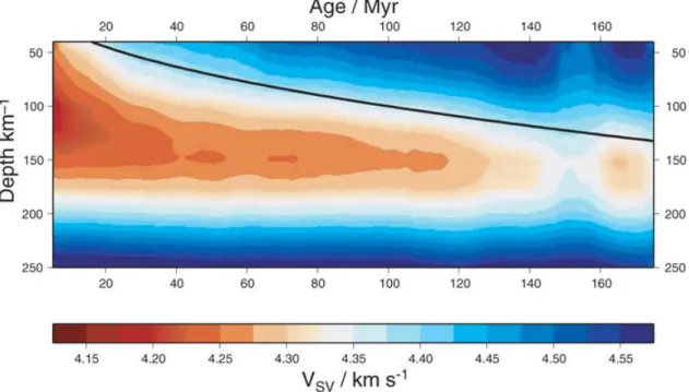
An intuitive image of the dependence of VSVon age can be found
in the age-dependent average cross-section for the Pacific Ocean lithosphere in Fig. 10, which was created by taking sliding window averages of our tomographic results at depths from 40 to 225 km along the isochrons of Fig. 9(b). Shear wave velocity in this image is expressed in absolute units for ease of comparison with other stud-ies and with physical models of the lithosphere. As tomographic inversions tend to underestimate the true amplitude of velocity per-turbations, the range of VSV at each depth may underestimate the
true range. The cross-section shows shear wave velocity decreasing with depth within the lithosphere down to∼150 km depth, where it reaches a minimum that goes from∼4.33 km s−1 at old ages
(>120 Ma) to ∼4.18 km s−1 at young ages (<20 Ma). The shear wave velocity of this low-velocity zone taken far from the ridge axis, is consistent with the results of Ekstr¨om & Dziewonski (1998) for the average VSV of the Pacific Plate. VSV contours in Fig. 10(a)
deepen progressively with age, approximately following the trend predicted by Parker & Oldenburg (1973) for purely diffusive cool-ing. The large oscillation for ages>140 Ma discussed for Fig. 9 is also present in this image. As the smoothing induced by the sliding window averaging procedure used to create this image precludes formal quantitative analysis of the observed VSV-age trend, such
analysis will be conducted below using non-overlapping age bins.
4 D I S C U S S I O N
4.1 Lithospheric cooling models
In the traditional oceanic plate tectonic model (e.g. Parsons & McKenzie 1978), new lithosphere is generated at mid-ocean ridges, the plates then cool, subside and thicken as they move away from the ridges, and the lithosphere reaches a stable state after∼60– 80 Myr. This model requires heat to be supplied to the base of older lithosphere, most probably by small scale convection, for it to stop cooling diffusively. A recent re-evaluation of the plate model by McKenzie et al. (2005) has found that the temperature depen-dence of thermal conductivity plays an important role in determining
Figure 10. Tomographic cross-section with respect to age for the Pacific Ocean region. This smoothed image was created by averaging VSValong the M¨uller et al. (1997) isochrons, using a sliding age window of 10 Ma width and excluding areas with no age information. Colour shading represents absolute VSV. The
continuous black line indicates the position of the thermal boundary layer for the Parker & Oldenburg (1973) half-space cooling model.
oceanic geotherms. Other models of lithospheric cooling include the half-space cooling model (Parker & Oldenburg 1973), in which the lithosphere is formed by diffusive cooling alone and continues to increase in thickness with age, and the recently revived constant heat-flux model (Crough 1975; Doin & Fleitout 1996), in which constant heat flow is assumed at the base of the lithosphere what-ever the age of the overlying plate. Discrimination between these cooling models and calibration of the plate model parameters (in particular mantle temperature and plate thickness) has tradition-ally been carried out using ocean depth and heat-flow data (e.g. Parsons & Sclater 1977; Stein & Stein 1992), although there have been efforts to include other data such as the geoid (Doin et al. 1996; DeLaughter et al. 1999). These surface observables, espe-cially oceanic topography and geoid, tend to reject the half-space cooling model in favour of plate models, but are not sufficiently accurate to distinguish between plate models and constant heat flow models (Doin & Fleitout 2000).
Seismological observables tell a different story. Nearly all studies of surface wave dispersion across the major ocean plates show that lithospheric seismic velocities, the thickness of the seismic litho-sphere and the seismic velocities in the low-velocity zone below the lithosphere all increase continuously with age when averaged over isochrons, and do not flatten out for older lithosphere as do the seafloor bathymetry and geoid (see Forsyth 1977; Zhang & Tanimoto 1991; Zhang & Lay 1999, for a review of the implications of sur-face wave phase dispersion observations on plate cooling models). These studies provide depth-dependent constraints on the cooling signature, while the traditional surface observations of bathymetry, heat flow or geoid are sensitive only to the integrated properties of the lithosphere. The seismological observations tend to favour the half-space conductive cooling model, or possibly a thick plate model (∼120 km thick) such as that of Parsons & Sclater (1977), over plate models with thin plates such as the widely recognized GDH1 model of Stein & Stein (1992). The reasons for which seismological and
surface observations seem incompatible are unclear, although the most likely candidates are uncertainties in the observations them-selves, especially the depth and heat flow observations at old ages. Insufficient path coverage in the central portions of the oceans adds uncertainty to the surface wave observations.
An exception to previous surface wave studies of lithospheric cooling is the recent study by Ritzwoller et al. (2004), who found a prominent flattening in the average VS-age trend for the Pacific
Ocean lithosphere between the ages of 70 and 100 Ma. They in-ferred a punctuated cooling history for the Pacific Ocean, with dif-fusive cooling being interrupted by reheating of 70 to 100 Myr old lithosphere, and suggested thermal boundary layer instabilities as a possible reheating mechanism. This observation is very different from those of previous surface wave studies of lithospheric cooling and also from current surface observations of bathymetry, heat flow and geoid, which all imply monotonic average cooling histories. If we compare the VSV-age trend from our study (Fig. 9) to that of
Ritzwoller et al. (2004) (Figure 5c from their paper), we find that instead of the prominent flattening between 70 and 100 Ma, we ob-serve mostly small amplitude oscillations of the VSVtrend with only
a very weak flattening signal. There may be multiple reasons for the discrepancy between our results and those of Ritzwoller et al. (2004). The most likely are differences in the surface wave data sets (which could lead to differences in surface wave coverage over the Pacific Ocean), the measurement techniques (secondary observables
vs. a combination of different phase and group velocity dispersion
techniques) and the tomographic inversion techniques (azimuthally anisotropic Gaussian ray tomography vs. radially anisotropic diffrac-tion tomography). The discrepancy is unlikely to be due simply to the use of ray theory compared with diffraction tomography (i.e. 2-D finite-frequency kernels), as Ritzwoller et al. themselves state that their result does not change significantly if they invert their phase and group velocity dispersion measurements using Gaussian ray theory instead of diffraction kernels.
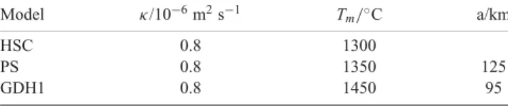
Table 1. Mantle parameters assumed by the three lithospheric cooling mod-els considered in this paper. HSC: half-space cooling model of Parker & Oldenburg (1973); PS: plate model of Parsons & Sclater (1977); GDH1: global depth and heat flow model of Stein & Stein (1992).
Model κ/10−6m2s−1 Tm/◦C a/km
HSC 0.8 1300
PS 0.8 1350 125
GDH1 0.8 1450 95
4.2 Comparison of VSV-age profiles with lithospheric
cooling models
We have compared our observed trend for VSVagainst ocean age to
three representative and well-known cooling models: the half-space cooling model of Parker & Oldenburg (1973) (hereafter referred to as HSC), the Parsons & Sclater (1977) plate model (hereafter referred to as PS) and the GDH1 plate model of Stein & Stein (1992). The mantle properties assumed by the three cooling models we considered are tabulated in Table 1. We assume that shear wave velocity VSV and temperature T are functions of age t and depth z
and are linearly related as follows:
VSV(t, z) − VSV(t0, z) VSV(t0, z)
= ∂lnVSV
∂T [T (t, z) − T (t0, z)], (1)
where t0 is a reference age and the partial derivative∂lnVSV/∂T
may depend on depth. We fit each of the cooling models to the observed VSVtrend at each depth, by allowing only∂lnVSV/∂T to
vary. Data for lithosphere younger than 10 Ma are excluded to avoid possible non-linearity in the temperature dependence of VSVdue to
the presence of partial melt or to diffusion boundary effects at the elevated temperatures near the ridge axis. We choose our reference age t0to be 10 Ma. We also exclude data for ages greater than 140
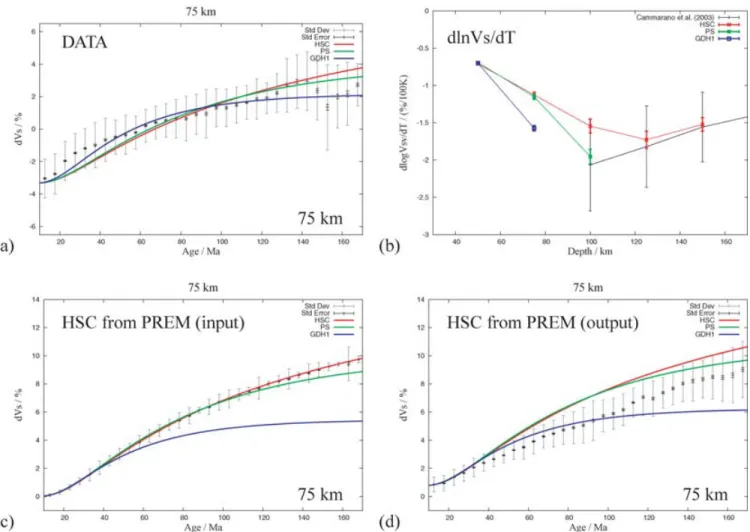
Ma in the fitting, although we do show the model predictions for older lithosphere. Fig. 11(a) shows the best-fit curves for the three cooling models at 75 km depth. All three lithospheric cooling models fit the binned tomographic values within their standard deviation, therefore, the tomography itself cannot formally rule out any of them. The best fit to the overall shape of the VSV-age trend is provided
by the Stein & Stein (1992) GDH1 plate model, while the HSC model and the PS thick plate model are almost indistinguishable in terms of goodness of fit. The robustness of this conclusion will be tested below.
The values of∂lnVSV/∂T obtained by the fitting of the three
models at depths up to 200 km are shown in Fig. 11(b), and com-pared with values determined from mineral physics experiments (Cammarano et al. 2003). As the temperature for the plate models is only defined within the plates themselves, we have not fitted these models to profiles at depths greater than their plate thickness. It is important to note that the absolute values of∂lnVSV/∂T we obtain
for each depth are lower bounds on the true absolute values, as the tomographic inversion is damped (via the a priori model variance
σM) towards a 1-D a priori model. A further illustration of the effect
of this damping is shown in the synthetic test below.
In order to test the robustness of any interpretation of the VSV
-age curves, we performed a synthetic tomographic experiment. We produced an input tomographic model starting from the smoothed PREM profile of Fig. 2, assuming a value of∂lnVSV/∂T of −1.5 per
cent/100 K, and imposing that the oceanic lithosphere had cooled according to the HSC model; we then computed the path-averaged shear wave velocity models along each of the 15 165 paths, and
imposed the same values ofσD used in the original inversion; we
then inverted this tomographic model under the same conditions as our real tomographic inversion, using as the a priori 1-D model the average velocity in the tomographic input model at each depth; fi-nally we binned both input and output synthetic tomographic mod-els in 5Ma age bins as described above. These VSV-age bins are
shown in Figs 11(c) and (d) for the input and output synthetic tomographic models, respectively. Comparison of the two panels shows that the range of VSVvalues is smaller for the output
tomo-graphic model, leading to the inference of a smaller ∂lnVSV/∂T
(1.0 per cent/100 K). More importantly, the shape of the output
VSV-age trend is distinctly different: it is flatter than that for the
input tomographic model between 60 and 100 Ma, it seems to be fit better by the GHD1 model than by the HSC model, and it dis-plays an oscillation that is similar to that observed for the real to-mographic model. In the synthetic test this oscillation is caused by reduced amplitude recovery of the tomography in the central Pacific region, itself caused most probably by uneven data cover-age and reduced lateral resolution in this same region (see Figs 4a and 5a).
The similarity in shape between the synthetic test output profile (Fig. 11d) and our tomographic profile (Fig. 11a) calls into ques-tion our earlier conclusion that a thin plate model provides the best fit to our surface wave observations, and suggests that a half-space cooling model or a thick plate model may be more appropriate, in accordance with most previous surface wave studies of litho-spheric cooling (Forsyth 1977; Zhang & Tanimoto 1991; Zhang & Lay 1999). The tendency of our tomographic inversion to flatten
VSV age profiles between 60 and 100 Ma makes us question the
large flattening signal observed by Ritzwoller et al. (2004). Such a signal is not strongly observed in our VSV age profiles despite
it being favoured by the path coverage as shown by our synthetic test. We cannot rule out that with better coverage of the Central Pacific region such a signal would indeed be robustly observed, and cannot test the path distribution used by Ritzwoller et al. directly. We, therefore, cannot robustly exclude the presence of a re-heating mechanism that may have affected the central Pacific lithosphere. However, we conclude from this synthetic tomographic experiment that detailed interpretation of the VSV-age trends from tomographic
images is likely to be misleading unless lateral resolution and ampli-tude recovery can be shown to be uniform across the oceanic region under consideration, a condition that is difficult to achieve in large oceanic basins with few seismic stations.
5 C O N C L U S I O N
In this study we have presented a multimode regional surface wave-form tomography of the Pacific upper mantle, using the two-stage method of secondary observables (Cara & L´evˆeque 1987; Debayle & Sambridge 2004) on over 56 000 Rayleigh wave paths. We have clustered these paths geographically with a cluster radius of 200 km in order to obtain a realistic estimate of the errors induced in wave-form modelling by inadequate knowledge of earthquake source pa-rameters. The preponderance of short path lengths in our data set has led to well-resolved images of the most densely covered re-gions, in particular of the Japan and Tonga-Kermadec subduction zones and of the West Pacific. Our improved coverage of the south-ern Pacific region thanks to data from the PLUME experiment of Barruol et al. (2002) has allowed us to determine that the low-velocity anomalies in the South Pacific Super-Swell region are con-fined to localized structures, and are not pervasive throughout the entire area.
Figure 11. (a) Fits of simple cooling models to average VSV-age profile at 75 km depth. VSVvalues are binned in 5 Ma bins, as in Fig. 9. For each bin, grey
error bars indicate the standard deviation and black error bars the standard error on the mean. Best-fit curves are shown for three models: HSC, half-space
cooling (Parker & Oldenburg 1973) in red; PS (Parsons & Sclater 1977) in green; GDH1 (Stein & Stein 1992) in blue. (b) Values of∂lnVSV/∂T obtained from
fitting the three cooling models to average VSV-age profiles at depths ranging from 50 to 150 km. Note that the two plate models (PS and GDH1) are only fitted
to the VSVobservations at depths that lie within each plate. (c) Fits of the three cooling models to a synthetic tomographic input model created by cooling the
PREM VSVmodel by half-space cooling. (d) Fits to the tomographic output model obtained by inverting the input model in (c) using the real data coverage and
tomographic inversion parameters.
We have produced an age-dependent average cross-section for the Pacific Ocean lithosphere, and interpreted the average VSV-age
profiles at different depths in terms of standard half-space cooling and plate cooling models. We have found that our tomography re-sults cannot rule out any of these models. Synthetic experiments suggest that geographical variations in amplitude resolution of the tomography due to insufficient path coverage in the central Pacific Ocean create an artificial flattening of the profile between 60 and 100 Ma. As increases in the path coverage of oceanic regions will be hard to obtain due to the difficulty and expense of deploying ocean bottom seismometers, we hope that further developments in tomographic techniques, for example the use of fully 3-D sensitivity kernels as described by Tromp et al. (2005), will bring about the im-provements in lateral resolution and amplitude recovery necessary for detailed seismological observation of geodynamic processes in oceanic regions.
A C K N O W L E D G M E N T S
A. Maggi was supported by a Marie Curie Individual Fellowship (contract HPMF-CT-2002-01636) from the European Union. The
study was also supported by the DyETI program ‘Imagerie globale et implications pour la dynamique de la zone de transition’ funded by the French Institut National des Sciences de l’Univers (INSU). The facilities of the IRIS Data Management System, and specifi-cally the IRIS Data Management Center, were used for access to waveform and metadata required in this study. The IRIS DMS is funded through the National Science Foundation and specifically the GEO Directorate through the Instrumentation and Facilities Pro-gram of the National Science Foundation under Cooperative Agree-ment EAR-0004370. Additional waveform data were obtained from the PLUME broadband deployment in the South Pacific, funded by the French Minist`ere de la Recherche, and facilitated by the Centre National de la Recherche Scientifique (CNRS), by the government of French Polynesia, and by the Universit´e de Polyn´esie fran¸caise (UPF). Supercomputer facilities were provided by the IDRIS na-tional centre in France. Most figures in this paper were prepared using the open source GMT software developed and maintained by Paul Wessel and Walter Smith, and supported by the NSF. The authors would like to thank Fabrice Fontaine and D. Reymond for supplying the PLUME data, and Mark Simons for suggesting the use of ORM.
R E F E R E N C E S
Barruol, G. et al., 2002. PLUME investigates the South Pacific Superswell,
EOS, Trans. Am. geophys. Un., 83, 511–514.
Bassin, C., Laske, G. & Masters, G., 2000. The current limits of resolution for surface wave tomography in North America, EOS, Trans. Am. geophys.
Un., 81, 897.
Beghein, C. & Trampert, J., 2004. Probability density functions for radial anisotropy from fundamental mode surface wave data and the neighbour-hood algorithm, Geophys. J. Int., 157, 1163–1174.
Beghein, C., Resovsky, J. & Trampert, J., 2002. P and S tomography using normal-mode and surface wave data with a neighbourhood algorithm,
Geophys. J. Int., 149(3), 646–658.
Boschi, L. & Ekstr¨om, G., 2002. New images of the Earth’s upper mantle
from measurements of surface wave phase velocity anomalies,J. Geophys.
Res., 107(B4), doi:10.1029/2000JB000059.
Cammarano, F., Goes, S., Vacher, P. & Giardini, D., 2003. Inferring upper-mantle temperatures from seismic velocities, Phys. Earth planet. Interiors, 138, 197–222, doi:10.1016/S0031-9201(03)00156-0.
Cara, M. & L´evˆeque, J., 1987. Waveform inversion using secondary observ-ables, Geophy. Res. Lett., 14, 1046–1049.
Courtillot, V., Davaille, A., Besse, J. & Stock, J., 2003. Three distinct types of hotspot in the Earth’s mantle, Earth planet. Sci. Lett., 205, 295– 308.
Crough, S., 1975. Thermal model of oceanic lithosphere, Nature, 256, 388– 390.
Debayle, E., 1999. Sv-wave azimuthal anisotropy in the Australian upper mantle: preliminary results from automated Rayleigh waveform inversion,
Geophys. J. Int., 137, 747–754.
Debayle, E. & Sambridge, M., 2004. Inversion of massive surface wave data sets: model construction and resolution assessment, J. geophys. Res., 109, doi:10.1029/2003JB002652.
Debayle, E., L´evˆeque, J.-J. & Cara, M., 2001. Seismic evidence for a deeply rooted low-velocity anomaly in the upper mantle beneath the northeastern Afro/Arabian continent, Earth planet. Sci. Lett., 193, 423–436. Debayle, E., Sambridge, M. & Priestley, K., 2005. Global azimuthal seismic
anisotropy and the unique plate–motion deformation of australia, Nature, 433, 509–512.
DeLaughter, J., Stein, S. & Stein, C., 1999. Extraction of a lithospheric cooling signal from oceanwide geoid data, Earth planet. Sci. Lett., 174, 173–181.
Doin, M. & Fleitout, L., 1996. Thermal evolution of the oceanic lithosphere: an alternate view, Earth planet. Sci. Lett., 142(1-2), 121–136.
Doin, M. & Fleitout, L., 2000. Flattening of the oceanic topography and geoid: thermal versus dynamic origin, Geophys. J. Int., 143, 582– 594.
Doin, M., Fleitout, L. & McKenzie, D., 1996. Geoid anomalies and the structure of continental and oceanic lithospheres, J. geophys. Res., 101(7), 16 119–16 135.
Dziewonski, A. M. & Anderson, D., 1981. Preliminary reference earth
model, Phys. Earth planet. Inter.,25(4), 297–356.
Ekstr¨om, G. & Dziewonski, A., 1998. The unique anisotropy of the Pacific upper mantle, Nature, 394, 168–172.
Ekstr¨om, G., Tromp, J. & Larson, E., 1997. Measurements and global models of surface wave propagtaion, J. geophys. Res., 102, 8137–8157. Forsyth, D., 1977. The evolution of the upper mantle beneath mid-ocean
ridges, Tectonophysics, 38, 89–118.
Gorbatov, A. & Kennett, B., 2003. Joint bulk-sound and shear tomography for Western Pacific subduction zones, Earth planet. Sci. Lett., 210, 527– 543.
Gung, Y., Panning, M. & Romanowicz, B., 2003. Global anisotropy and the thickness of continents, Nature, 422, 707–711.
Lebedev, S. & Nolet, G., 2003. Upper mantle beneath southeast Asia from S velocity tomography, J. geophys. Res., 108(B1), doi:10.1029/2000JB000073.
L´evˆeque, J., Debayle, E. & Maupin, V., 1998. Anisotropy in the Indian Ocean upper mantle from Rayleigh and Love waveform inversion, Geophys. J.
Int., 133, 529–540.
Levshin, A., Barmin, M., Ritzwoller, M. & Trampert, J., 2005. Minor-arc and major-arc global surface wave diffraction tomography, Phys. Earth
planet. Inter., 149, 205–223.
Maggi, A. & Priestley, K., 2005. Surface waveform tomography of the Turk-ish Iranian plateau, Geophys. J. Int., 160(3), 1068–1080.
Maggi, A., Debayle, E. & Priestley, K., 2006. Azimuthal anisotropy of the Pacific Ocean upper mantle, Earth planet. Sci. Lett., (in press). McKenzie, D., Jackson, J. & Priestley, K., 2005. Thermal structure of
oceanic and continental lithosphere, Earth planet. Sci. Lett., 233, 337– 349.
McNutt, M. & Fischer, K., 1987. The South Pacific superswell, in Seamounts,
Islands, and Atolls, Vol. 43, pp. 25–34, eds Keating, B. H. Fryer, P. Batiza,
R. & Boehlert, G.W., of Geophysical Monograph, American Geophysical Union, Washington, DC.
M´egnin, C. & Romanowicz, B., 2000. The three-dimensional shear velocity structure of the mantle from the inversion of body, surface and higher-mode waveforms, Geophys. J. Int., 143, 709–728.
Montagner, J.-P., 1986. Regional three-dimensional structures using long-period surface waves, Ann. Geophys., 4, 283–294.
Montagner, J.-P., 2002. Upper mantle low anisotropy channels below the Pacific Plate, Earth planet. Sci. Lett., 202, 263–274.
Montagner, J.-P. & Tanimoto, T., 1991. Global upper mantle tomogra-phy of seismic velocites and anisotropies, J. geotomogra-phys. Res., 96, 20 337– 20 351.
Mooney, W., Laske, G. & Masters, G., 1998. Crust 5.1: a global crustal model at 5x5 degrees, J. geophys. Res., 103, 727–747.
M¨uller, R., Roest, W., Royer, J.-Y., Gahagan, L. & Sclater, J., 1997. Digital isochrons of the world’s ocean floor, J. geophys. Res., 102(B2), 3211– 3214.
Nataf, H. & Ricard, Y., 1995. 3SMAC: an a priori tomographic model of the upper mantle based on geophysical modeling, Phys. Earth planet. Inter., 95, 101–122.
Nishimura, C. & Forsyth, D., 1988. Rayleigh wave phase velocities in the Pacific with implications for azimuthal anisotropy and lateral hetero-geneities, Geophys. J., 94, 479–501.
Nishimura, C. & Forsyth, D., 1989. The anisotropic structure of the upper mantle in the Pacific, Geophys. J., 96, 203–229.
Parker, R. & Oldenburg, D., 1973. Thermal model of ocean ridges, Nature, 242, 137–139.
Parsons, B. & McKenzie, D., 1978. Mantle convection and thermal structure of the plates, J. geophys. Res., 83, 4485–4496.
Parsons, B. & Sclater, J., 1977. An analysis of the variation of ocean floor bathymetry and heat flow with age, J. geophys. Res., 82, 803–827. Pilidou, S., Priestley, K., Gudmundsson, O. & Debayle, E., 2004. Upper
mantle s-wave speed heterogeneity and anisotropy beneath the north at-lantic from regional surface wave tomography: the Iceland and Azores plumes, Geophys. J. Int., 159(3), 1057–1076.
Priestley, K. & Debayle, E., 2003. Seismic evidence for a moderately thick lithosphere beneath the Siberian Platform, Geophy. Res. Lett., 30(3), doi:10.1029/2002GL015931.
Richardson, W., Okal, E. & Van der Lee, S., 2000. Rayleigh-wave tomogra-phy of the Ontong–Java Plateau, Phys. Earth planet. Inter., 111, 29–51. Ritsema, J. & Allen, R., 2003. The elusive mantle plume, Earth planet. Sci.
Lett., 207, 1–12.
Ritsema, J., van Heijst, H. & Woodhouse, J., 1999. Complex shear wave velocity structure imaged beneath Africa and Iceland, Science, 286, 1925– 1928.
Ritsema, J., van Heijst, H. & Woodhouse, J., 2004. Global transition zone tomography, J. geophys. Res., 106(B02302), doi:10.1029/2003JB002610. Ritzwoller, M., Shapiro, N., Barmin, M. & Levshin, A., 2002. Global surface wave diffraction tomography, J. geophys. Res., 107(B12), 10.1029/2002JB001777.
Ritzwoller, M., Shapiro, N. & Zhong, S.-J., 2004. Cooling history of the Pacific lithosphere, Earth planet. Sci. Lett., 226, 69–84.
Sichoix, L., Bonneville, A. & McNutt, M., 1998. The seafloor swells and Su-perswell in French Polynesia, J. geophys. Res., 103(B11), 27 123–27 133. Sieminski, A., Debayle, E. & L´evˆeque, J.-J., 2003. Seismic evidence for deep low-velocity anomalies in the transition zone beneath Western
Antarctica, Earth planet. Sci. Lett., 216, 645–661, doi:10.1016/S0012-821X(03)00518-1.
Sieminski, A., L´evˆeque, J.-J. & Debayle, E., 2004. Can finite-frequency effects be accounted for in ray theory surface wave tomography?, Geophys.
Res. Lett., 31, doi:10.1029/2004GL021402.
Smith, W. & Sandwell, T., 1997. Global seafloor topography from satellite altimetry and ship depth soundings, Science, 277, 1956–1962. Smith, D., Ritzwoller, M. & Shapiro, N., 2004. Stratification of
anisotropy in the Pacific upper mantle, J. geophys. Res., 109, doi:10.1029/2004JB003200.
Spetzler, J. & Snieder, R., 2001. The effect of small-scale heterogeneity on the arrival time of waves, Geophys. J. Int., 145, 786–796.
Stein, C. & Stein, S., 1992. A model for the global variation in oceanic depth and heat flow with lithospheric age, Nature, 359, 123–129.
Tarantola, A. & Valette, B., 1982. Generalised nonlinear inverse prob-lems solved using the least square criterion, Rev. Geophys., 20, 219– 232.
Tommasi, A., Godard, M., Coromina, G., Dautria, J. & Barsczus, H., 2004. Seismic anisotropy and compositionally induced velocity anomalies in
the lithosphere above mantle plumes: a petrological and microstructural study of mantle xenoliths from French Polynesia, Earth planet. Sci. Lett., 227, 539–556.
Trampert, J. & Woodhouse, J., 2003. Global anisotropic phase velocity maps for fundamental mode surface waves between 40 and 150 s, Geophys. J.
Int., 154, 154–165.
Tromp, J., Tape, C. & Liu, Q., 2005. Seismic tomography, adjoint methods, time reversal and banana-doughnut kernels, Geophys. J. Int., 160, 195– 216.
Van Heijst, H. & Woodhouse, J., 1999. Global high-resolution phase veloc-ity distributions of overtone and fundamental-mode surface waves deter-mined by mode branch stripping, Geophys. J. Int., 137, 601–620. Yoshizawa, K. & Kennett, B., 2002. Determination of the influence zone for
surface wave paths, Geophys. J. Int., 149, 440–453.
Zhang, T. & Lay, T., 1999. Evolution of oceanic upper mantle structure,
Phys. Earth planet. Inter., 114, 71–80.
Zhang, Y.-S. & Tanimoto, T., 1991. Global Love wave phase velocity varia-tion and its significance to plate tectonics, Phys. Earth planet. Inter., 66, 160–202.