HAL Id: hal-00302992
https://hal.archives-ouvertes.fr/hal-00302992
Submitted on 22 Apr 2008
HAL is a multi-disciplinary open access
archive for the deposit and dissemination of
sci-entific research documents, whether they are
pub-lished or not. The documents may come from
teaching and research institutions in France or
abroad, or from public or private research centers.
L’archive ouverte pluridisciplinaire HAL, est
destinée au dépôt et à la diffusion de documents
scientifiques de niveau recherche, publiés ou non,
émanant des établissements d’enseignement et de
recherche français ou étrangers, des laboratoires
publics ou privés.
investigation using nonlinear dimensionality reduction
I. Ross, P. J. Valdes, S. Wiggins
To cite this version:
I. Ross, P. J. Valdes, S. Wiggins. ENSO dynamics in current climate models: an investigation using
nonlinear dimensionality reduction. Nonlinear Processes in Geophysics, European Geosciences Union
(EGU), 2008, 15 (2), pp.339-363. �hal-00302992�
© Author(s) 2008. This work is licensed
under a Creative Commons License.
in Geophysics
ENSO dynamics in current climate models: an investigation using
nonlinear dimensionality reduction
I. Ross1, P. J. Valdes1, and S. Wiggins2
1School of Geographical Sciences, University of Bristol, University Road, Bristol BS8 1SS, UK 2School of Mathematics, University of Bristol, University Walk, Bristol BS8 1TW, UK
Received: 9 October 2007 – Revised: 18 February 2008 – Accepted: 26 March 2008 – Published: 22 April 2008
Abstract. Linear dimensionality reduction techniques, no-tably principal component analysis, are widely used in cli-mate data analysis as a means to aid in the interpretation of datasets of high dimensionality. These linear methods may not be appropriate for the analysis of data arising from nonlinear processes occurring in the climate system. Nu-merous techniques for nonlinear dimensionality reduction have been developed recently that may provide a potentially useful tool for the identification of low-dimensional mani-folds in climate data sets arising from nonlinear dynamics. Here, we apply Isomap, one such technique, to the study of El Ni˜no/Southern Oscillation variability in tropical Pacific sea surface temperatures, comparing observational data with simulations from a number of current coupled atmosphere-ocean general circulation models. We use Isomap to exam-ine El Ni˜no variability in the different datasets and assess the suitability of the Isomap approach for climate data analysis. We conclude that, for the application presented here, anal-ysis using Isomap does not provide additional information beyond that already provided by principal component analy-sis.
1 Introduction
The El Ni˜no/Southern Oscillation (ENSO) is the most im-portant mode of interannual variability in the Earth’s climate, driven by atmosphere-ocean interactions in the equatorial Pa-cific, but with effects reaching as far as north-eastern North America and Europe (Philander, 1990; McPhaden et al., 2006). ENSO events (El Ni˜no and La Ni˜na) occur on an ir-regular basis at intervals of 2–7 years, and individual ENSO events are variable in their evolution and effects. As a re-cent example, the 1997/1998 El Ni˜no exhibited behaviour not previously seen, with westerly wind bursts linked to the Madden-Julian Oscillation playing an important role; some Correspondence to: I. Ross
observers have suggested that this may represent a transition to a new regime of ENSO behaviour (McPhaden, 1999; Fe-dorov and Philander, 2000).
The representation of ENSO in climate models is of inter-est because of the long-range effects of ENSO on the climate system, both around the Pacific and further afield. Recent model intercomparison studies considering ENSO variabil-ity in the current generation of coupled atmosphere-ocean general circulation models (AchutaRao and Sperber, 2002, 2006; van Oldenborgh et al., 2005; Guilyardi, 2006) indicate that some aspects of ENSO variability are represented bet-ter in current models than in earlier generations of GCMs (Neelin et al., 1992; Latif et al., 2001), including the over-all frequency of El Ni˜no events and enhanced temperature variability over the eastern Pacific. However, current mod-els still display significant deficiencies in the representation of the ocean-atmosphere coupling mechanisms important for ENSO variability – see particularly van Oldenborgh et al. (2005) on this point, where the individual feedback mecha-nisms relating wind stress, thermocline depth and sea surface temperature are examined in detail in current models.
There has been considerable disagreement about the ex-act source of ENSO variability. One point of view is that ENSO arises from unstable modes of variability in the trop-ical ocean-atmosphere system, with limits to predictability determined by growth in errors in initial conditions associ-ated with chaotic dynamics (e.g., Zebiak and Cane, 1987; Jin et al., 1994; Tziperman et al., 1994). The other possibility is that ENSO is a damped linear oscillation excited by stochas-tic forcing, the limits to predictability being inherent in the stochastic nature of the forcing (e.g., Burgers, 1999; Moore and Kleeman, 1999; Thompson and Battisti, 2000). One de-ficiency of linear models is that they are not able to repro-duce the observed asymmetry between El Ni˜no and La Ni˜na events. This asymmetry has previously been investigated using measures based on sea surface temperature (SST) vari-ance and skewness, nonlinear dynamical heating and explicit characterisation of symmetric and asymmetric structures in
SSTs during ENSO events (An, 2004; An and Jin, 2004; An et al., 2005a; Monahan and Dai, 2004). These studies reveal wide variations in the representation of ENSO asymmetry in coupled ocean-atmosphere models.
Independent of the exact mechanism of variability, the spatial coherence of ENSO in the Pacific leads us to ex-pect that there should be a low-dimensional model that cap-tures at least some of the variability in the tropical ocean-atmosphere system. Here, we approach the assessment of ENSO in coupled GCMs by attempting to identify such low-dimensional structures in the dynamics of the tropical Pacific atmosphere and ocean. It should be noted that, in general, the mechanisms leading to ENSO and ENSO-like variabil-ity in current coupled atmosphere-ocean GCMs show sig-nificant differences compared to the mechanisms contribut-ing to ENSO variability in the real atmosphere-ocean sys-tem. For instance, van Oldenborgh et al. (2005) report that most of the models that they examine show a response of the zonal wind field to equatorial SST anomalies that is weaker and more confined to equatorial latitudes than seen in ob-servations. This weak wind response is compensated by a stronger direct response of SSTs to changes in the wind field and a weaker damping of SST variations than observed. This different balance of factors in the models compared to the observations should lead us to view conclusions drawn from models about ENSO variability in the real atmosphere and ocean with some caution. However, it is still of interest to examine how well we can characterise what low-dimensional dynamics is seen in the models, and to see if this character-isation can provide any further insight into the behaviour of the models. For instance, earlier studies have indicated that ENSO variability can be approximated as a two-dimensional oscillation, one degree of freedom being associated with the NINO3 SST index, the mean SST anomaly across the region 150◦W–90◦W, 5◦S–5◦N, and the other with the equatorial Pacific warm water volume (Burgers, 1999; Kessler, 2002; McPhaden, 2003). These two degrees of freedom vary in approximate quadrature during El Ni˜no events. One would hope that any analysis method aimed at characterising ENSO variability in observational or simulated data would be able to identify these two degrees of freedom.
Our question here is, given high-dimensional data from observations or model simulations, what is the best way to characterise low-dimensional behaviour? We are interested in attempting to infer low-dimensional dynamics from rel-atively limited amounts of data. Observational time series from the Pacific provide around 100 years of monthly SSTs. Time series of several hundred years are available from cou-pled GCM simulations. To facilitate inter-model compari-son, we wish to proceed in a “black box” fashion, adopting a purely data-driven approach without using information about the internal features of the models we are studying.
The method most commonly used in climate data analysis for this type of dimensionality reduction is principal compo-nent analysis (PCA) (von Storch and Zwiers, 2003), which
uses an eigendecomposition of the input data covariance ma-trix. In the problem considered here, we analyse a time se-ries of n maps of sea surface temperature, each with m ocean points. Discarding non-ocean points in each map, we use SST measurements from the remaining ocean data points to construct data vectors xi ∈ Rm, with i=1, . . ., n. The
co-variance matrix of this SST data is then C = h(x − hxi)(x − hxi)Ti,
where h·i denotes time averaging. We write the eigenvector decomposition of C as C=Q3QT, with
3= diag(λ1, . . . , λm) a diagonal matrix of the eigenvalues
λi in descending order of magnitude, and Q a matrix whose
columns are the corresponding eigenvectors qi. The
eigen-vectors qi ∈ Rmare spatial patterns of variation in the data,
often called empirical orthogonal functions (EOFs). The first of these, q1, represents the direction in data space with the
greatest variance, q2the direction orthogonal to q1with the
next greatest variance in the data, and so on. The time se-ries of SST maps, xi, can then be expanded in terms of the
orthogonal basis provided by the EOFs as
xi =
X
j
αijqj.
The coefficients αij are called the principal component (PC)
time series and give the temporal variation in the data in each of the orthogonal directions in data space spanned by the EOFs. The eigenvalue associated with each EOF measures the proportion of the total variance of the in-put data explained by that EOF. With the EOFs in de-scending eigenvalue order, we may extract an EOF sub-set explaining some pre-selected proportion of the total variance, Vp={qi|1≤i≤p} say, where p is the number of
EOFs required to explain the required proportion of the to-tal variance. By projecting the input data into the subspace
Vp= span(Vp), we arrive at a reduced dimensionality
repre-sentation of variability in the input data. Compared to the original data this reduced representation has the minimum squared error totalled over all data points of any choice of projection basis of dimension p.
The primary disadvantage of PCA for our purposes is that it is only able to project into linear subspaces of the original
m-dimensional data space. If our data points, instead of lying
in a linear subspace, lie in a curved low-dimensional sub-manifold of the data space, PCA will generally not detect the full structure of the data manifold, instead approximating it by the nearest linear subspace in a least squares sense.
This limitation has led to the development of a wide range of nonlinear dimensionality reduction approaches. Of these schemes, only a small number have previously been applied to ENSO data. These include both the method used in this study (Tenenbaum et al., 2000; G´amez et al., 2004) and meth-ods based on neural networks, either self-organising maps (Leloup et al., 2007) or multilayer perceptrons (Monahan, 2001; An et al., 2005b; Wu and Hsieh, 2003).
The neural network approach that has seen most applica-tion to quesapplica-tions of ENSO variability is nonlinear princi-pal component analysis (NLPCA), described by Monahan (2001) and, including extensions to canonical correlation analysis and singular spectral analysis, Hsieh (2004). The NLPCA method uses an autoassociative neural network hav-ing input and output layers with numbers of neurons cor-responding to the number of dimensions of the input data (a preliminary projection into the space spanned by the first few EOFs is normally used to reduce the dimensionality of the input data without losing a significant amount of the data variance), hidden layers attached to the input and output lay-ers with as many neurons as required to give a good fit to the input data, and a “bottleneck layer” between the two hid-den layers, whose architecture determines the form of the re-duced dimensionality data prore-duced. The neural network is trained on the data set whose dimensionality is to be reduced, the weights in the network being varied so as to reduce the mean squared error between the input data (applied to the in-put layer of the network) and the network outin-puts. The idea is thus to produce a network reproducing the input data as faithfully as possible, with information passing through the bottleneck layer, which has a restricted number of neurons. The outputs of the neurons in the bottleneck layer are then taken to be a reduced dimensionality representation of the input data. A single neuron in the bottleneck layer produces a one-dimensional reduced representation of the input data, two neurons in the bottleneck layer a two-dimensional re-duced representation, and so on. Additional constraints can be imposed on the structure of the bottleneck layer to yield reduced representations with required characteristics. The most obvious example of this is a “circular” bottleneck node, with two degrees of freedom whose values are constrained to define a point on the unit circle. This yields a bottleneck layer representing a periodic one-dimensional system. Application of NLPCA with one- and two-dimensional bottleneck layers to tropical Pacific observational SST data demonstrated that low-dimensional NLPCA approximations characterise vari-ability in the data better than the corresponding linear PCA approximations, and that NLPCA approximations are able to represent the asymmetry between El Ni˜no and La Ni˜na seen in the observational data (Monahan, 2001). Applica-tion of NLPCA with a circular bottleneck layer to observa-tional thermocline depth data from the equatorial Pacific suc-cessfully captured the oscillatory nature of thermocline depth variations through the ENSO cycle, and identified differ-ences in the behaviour of the recharge and discharge phases of the oscillation (An et al., 2005b). Further applications of NLPCA in the context of studies of ENSO include the use of nonlinear canonical correlation analysis (NLCCA) to iden-tify nonlinear correlations between SST and wind stress vari-ations in the equatorial Pacific (Wu and Hsieh, 2003).
Many other nonlinear dimensionality reduction techniques have been developed, mostly in the machine vision com-munity, to address issues of feature identification and
mo-tion tracking (e.g., Bishop et al., 1998; Roweis and Saul, 2000; Broomhead and Kirby, 2005; Hinton and Salakhutdi-nov, 2006; Lin et al., 2006). Many of these methods can be placed into a common framework along with PCA by con-sidering them as seeking a transformation that preserves “in-teresting” geometric information in the input data. In the case of PCA, this “interesting” information is the Euclidean distances between data points; the required transformation is thus a simple linear orthogonal transformation. A more complex example is the algorithm used in this study, Isomap (Tenenbaum et al., 2000). Isomap finds a nonlinear transfor-mation that preserves not Euclidean distances between data points, but an approximation to distances between data points as measured along geodesics in the data manifold. These geodesic distances are an intrinsic feature of the dynamics of the system under study and are not dependent on the details of the embedding in the observation space. Further elabora-tions of this idea are possible. For instance, Lin et al. (2006) introduce a method they call Riemannian Manifold Learn-ing, which attempts to preserve not only an approximation to geodesic distances in the data manifold, but also local curva-ture information. We do not consider this method further in this study.
The only previous application of Isomap to climate data analysis of which we are aware is the work of G´amez et al. (2004), where Isomap was applied to observational SSTs for the equatorial Pacific to examine ENSO variability. G´amez et al.’s results are substantially replicated by our raw SST analysis of the NOAA ERSST v2 observational dataset (Sect. 5.1) and we extend their analysis to consider results from coupled atmosphere-ocean GCMs. As well as being of intrinsic interest, ENSO variability provides a good test case for nonlinear dimensionality reduction methods, primarily because the expected results are relatively easy to interpret. ENSO is by far the strongest mode of climate variability after the annual cycle and has both a clear signature of temporal variability and easily recognisable spatial patterns.
The plan of the paper is as follows. In Sect. 2, we describe the datasets we use. In Sect. 3, we present some conventional analyses of ENSO behaviour in the model simulations to set the scene for interpretation of the Isomap results. In Sect. 4, we describe the Isomap algorithm and examine some issues relating to the sensitivity of Isomap to tunable parameters in the algorithm. Section 5 presents results from performing Isomap analyses on tropical Pacific SST datasets. Finally, in Sect. 6, we present conclusions and recommendations con-cerning the use of Isomap in climate data analysis.
2 Data and models
In this study, we examine ENSO variability in tropical Pa-cific SST data from a variety of observational and model sources. Since ENSO is a coupled ocean-atmosphere phe-nomenon, it would be better to examine other variables in
conjunction with SST, in particular thermocline depth and surface wind stress. However, our goal here is to perform a simple inter-model comparison, so we initially restrict our analysis to SST. We include some analysis of thermocline depth variations later, mostly in the form of equatorial warm water volume.
As observational SST data, we use the NOAA ERSST v2 dataset (Smith and Reynolds, 2004). This is a global dataset running from 1854 to the present day at 2◦×2◦ resolution, constructed from SST observations using statistical recon-structions in regions with sparse observations. Because of a lack of observations in the equatorial Pacific before about 1900, most variability in this region in the early part of the time series is due solely to the annual cycle. For the pur-poses of this study, we extract a 100-year subset from 1900– 1999 of the full ERSST v2 time series in order to reduce problems due to non-stationarity. There is still some resid-ual non-stationarity in the SST observations associated with changes in ENSO behaviour over time, but this is small. We also examined another observational SST dataset covering a comparable period, the UK Meteorological Office HadISST 1.1 dataset (UK Meteorological Office, 2006). Results were similar to those reported here. In Sects. 5.1 and 5.2, we ex-amine correlations between Isomap results and equatorial Pa-cific warm water volume (WWV) time series. For observa-tional WWV data, we use the time series derived by Meinen and McPhaden (2000).
Model simulations from a range of coupled ocean-atmosphere GCMs were used for this study, utilising results from the World Climate Research Programme’s (WCRP) Coupled Model Intercomparison Project phase 3 (CMIP3) multi-model dataset (Table 1). In this study, we use data from pre-industrial control simulations (picntrl) in the CMIP3 database. We do not use all of the CMIP3 models, excluding from consideration simulations that show little or no interannual tropical Pacific atmosphere-ocean variability, either because of the model structure or due to other uniden-tified problems (e.g., the GISS-AOM and GISS-ER models). For all model simulations, monthly SST time series are used, the length of the time series available for each model being shown in Table 1. Warm water volume time series were cal-culated for all models where ocean body temperature data was available by determining the depth of the 20◦C isotherm by linear interpolation, then integrating the volume of water above the 20◦C isotherm in the region 120◦E–80◦W, 5◦S– 5◦N, as in McPhaden (2003).
3 Model ENSO behaviour
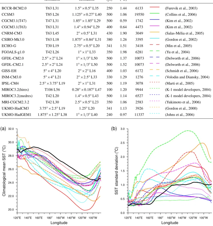
Before considering Isomap, we present some more con-ventional analyses of ENSO behaviour. First, we consider the climatology and magnitude of interannual variability of equatorial Pacific SSTs. Figure 1a shows annual mean SST in the equatorial Pacific, averaged between 2◦S and 2◦N.
Al-though most of the models show a cold bias across the Pacific basin, with SSTs up to 4◦C cooler than observed, they do simulate the gradient of mean SST from the Western Warm Pool around Indonesia to the cooler waters of the eastern Pa-cific. However, most of the models do not show a monotonic eastwards decline in SST across the basin, instead exhibit-ing an upturn in mean SST from 100–120◦W to the east-ern edge of the basin. These warmer temperatures near the eastern basin boundary have been observed in previous inter-model comparisons of tropical Pacific SST variability (Me-choso et al., 1995; Latif et al., 2001; AchutaRao and Sperber, 2002) and have been ascribed to difficulties in modelling ma-rine stratus clouds in this region, the steep orography near the coast of South America and the narrow coastal upwelling zone in the eastern Pacific. It appears that relatively little progress has been made in correcting this deficiency in cur-rent coupled GCMs.
Figure 1b shows the annual standard deviation of SST across the Pacific in the same latitude band. Here, observa-tions show low variability in the western Pacific and higher variability in the east, where conditions vacillate between the normal cold tongue state and El Ni˜no conditions, char-acterised by the incursion of warmer water from the west-ern Pacific into the east. Some of the models represent this pattern reasonably well, although the gradient in variabil-ity is represented less well than the gradient in mean SST, and again there are problems for all of the models at the far eastern end of the Pacific basin, probably for the same rea-sons as for the mean SST. The range of variability of the modelled SSTs is quite wide, with one model (FGOALS-g1.0) showing variability as much as 2.5 times the observed values. Some models (CGCM3.1(T47), CGCM3.1(T63), MIROC3.2(hires) and MIROC3.2(medres)) simulate essen-tially no gradient in variability across the basin.
The SST variability data displayed in Fig. 1b can be sum-marised using the NINO3 SST index. High values of this index reflect El Ni˜no conditions and low values La Ni˜na con-ditions. The fifth column of Table 1 shows the standard de-viation of the NINO3 SST index for each of the models used here. For comparison, the standard deviation of NINO3 SST for the ERSST v2 observational dataset is 1.26◦C for the pe-riod 1900–2000. The results in Table 1 indicate that most of the models have a reasonable range of NINO3 SST vari-ability, with CGCM3.1(T47), CGCM3.1(T63) and UKMO-HadGEM1 having too little variability and CNRM-CM3 and FGOALS-g1.0 too much. (As noted above, a number of other models in the CMIP3 model inter-comparison were not used in this study because of unrealistically low NINO3 SST vari-ability. Only models with a NINO3 SST standard deviation of 0.5◦C or greater were included in this study.)
The temporal variability of ENSO can be examined us-ing power spectra of the NINO3 SST anomaly time series. Figure 2 shows such spectra calculated using a maximum entropy method (Press et al., 1992, Sect 13.7). The observa-tions show a broad and low peak for periods between about
Table 1. Models used in this study, atmosphere and equatorial ocean spatial resolutions, lengths of simulation available (L), NINO3 SST
index standard deviations (σNINO3), number of ocean grid points in the region 125◦W–65◦W, 20◦S–20◦N (m), line style used in later plots
and references to model documentation. Model horizontal resolution is expressed as degrees longitude × degrees latitude or a spectral grid designation and vertical resolution as Ln, where n is the number of model levels.
Model Atmosphere Ocean L σNINO3 m Legend Reference resolution resolution (yr) (◦C)
BCCR-BCM2.0 T63 L31 1.5◦×0.5◦L35 250 1.44 6133 (Furevik et al., 2003) CCSM3 T85 L26 1.125◦×0.27◦L40 500 1.06 19550 (Collins et al., 2006) CGCM3.1(T47) T47 L31 1.85◦×1.85◦L29 500 0.59 1742 (Kim et al., 2002) CGCM3.1(T63) T63 L31 1.4◦×0.94◦L29 400 0.64 4473 (Kim et al., 2002) CNRM-CM3 T63 L45 2◦×0.5◦L31 430 1.90 3049 (Salas-M´elia et al., 2005) CSIRO-Mk3.0 T63 L18 1.875◦×0.84◦L31 380 1.26 3395 (Gordon et al., 2002) ECHO-G T30 L19 2.75◦×0.5◦L20 341 1.51 3418 (Min et al., 2005) FGOALS-g1.0 T42 L26 1◦×1◦L33 350 1.98 6281 (Yu et al., 2004) GFDL-CM2.0 2.5◦×2◦L24 1◦×1/3◦L50 500 1.37 10073 (Delworth et al., 2006) GFDL-CM2.1 2.5◦×2◦L24 1◦×1/3◦L50 500 1.52 10073 (Delworth et al., 2006) GISS-EH 5◦×4◦L20 2◦×2◦L16 400 1.03 6172 (Schmidt et al., 2006) INM-CM3.0 5◦×4◦L21 2◦×2.5◦L33 330 1.29 1276 (Volodin and Diansky, 2004) IPSL-CM4 2.5◦×3.75◦L19 2◦×1◦L31 500 1.19 3078 (Marti et al., 2005)
MIROC3.2(hires) T106 L56 0.28◦×0.187◦L47 100 1.20 9944 (K-1 model developers, 2004) MIROC3.2(medres) T42 L20 1.4◦×0.5◦L43 500 1.14 6527 (K-1 model developers, 2004) MRI-CGCM2.3.2 T42 L30 2.5◦×0.5◦L23 350 1.06 2583 (Yukimoto et al., 2006) UKMO-HadCM3 3.75◦×2.5◦L19 1.25◦L20 341 1.13 3926 (Gordon et al., 2000) UKMO-HadGEM1 1.875◦×1.25◦L38 1◦×1/3◦L40 240 0.97 11337 (Johns et al., 2006)
Fig. 1. Climatological mean SST (a) and annual standard deviation of SST (b) across the equatorial Pacific from observations (thick black
Fig. 2. Maximum entropy power spectra of NINO3 SST index
vari-ability from observations (thick black line) and models (coloured lines – see Table 1 for key). All spectra are calculated using 20 poles.
2 and 7 years, indicating the temporal irregularity of ENSO. Among the models, this pattern is replicated most closely in the GFDL-CM2.1, INM-CM3.0 and UKMO-HadCM3 sim-ulations. Other models show either weaker variability in the ENSO band, or variability that is too strongly peaked around a single frequency. This is particularly evident for CCSM3, CNRM-CM3, ECHO-G and FGOALS-g1.0. For the more extreme of these models, one can question whether these narrowband signals can really be identified with ENSO, since they lack the characteristic broad power spectrum of observed ENSO variability.
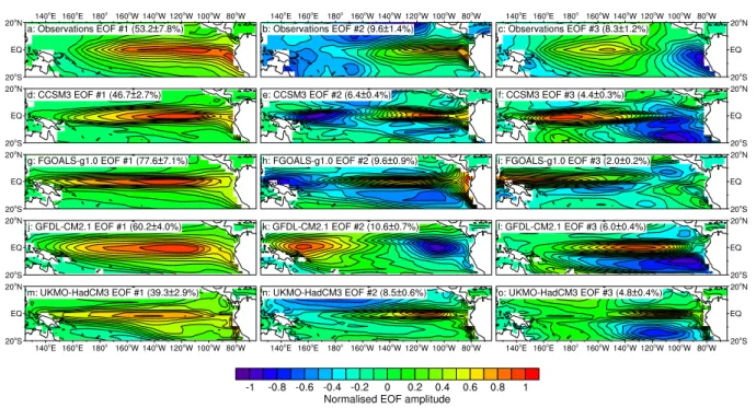
A common linear dimensionality reduction approach used for geophysical and climate data analysis is principal com-ponent analysis (PCA) (von Storch and Zwiers, 2003), also known as empirical orthogonal function (EOF) analysis. The relationship between this linear method and the nonlinear Isomap method will be explored in Sect. 4, but here we present some PCA results for our SST datasets. We calcu-lated area weighted EOFs and principal component time se-ries for SST anomalies from all datasets across the region 125◦W–65◦W, 20◦S–20◦N. For the observed ERSST v2 SSTs, we used data for the period 1900-2000, while for the models, we used all of the available output, with simulation lengths as listed in Table 1. In each case, after computation, the EOFs are normalised to have unit maximum amplitude for ease of plotting. The corresponding principal component time series are rescaled accordingly.
The first three EOFs from the observations are shown in Figs. 3a–c. The first EOF (Fig. 3a) shows a SST pattern sub-stantially similar to that of a fully developed El Ni˜no event, with warmer temperatures stretching across the equatorial Pacific, replacing the normal tongue of cooler water lying in the eastern Pacific. This first EOF explains 53.2% of the total
variance in the SST data. The second EOF (Fig. 3b) shows a northwest-southeast oriented dipole pattern centred around 120◦W, 10◦N, explaining about 9.5% of the total observed variance, while the third EOF (Fig. 3c) explains 8.3% of the data variance and shows an east-west dipole lying along the equator with centres of action at around 160◦W and near the coast of South America.
These patterns of observed spatial variability can be com-pared to results from the model simulations. Some se-lected results are shown in Figs. 3d–o. Here, we display the first three EOFs for CCSM3 (Figs. 3d–f), FGOALS-g1.0 (Figs. 3g–i), GFDL-CM2.1 (Figs. 3j–l) and UKMO-HadCM3 (Figs. 3m–o). The patterns seen represent a cross-section of the typical behaviour seen in the models. In each case, the first EOF is of approximately the right shape, but stretches too far to the west across the Pacific. In the ob-served data, the region of greatest weight in the first EOF lies well to the east of the date line, while in the model re-sults it extends westwards to 150◦E or further. Also, only the pattern for GFDL-CM2.1 has a reasonable shape in the far eastern sector of the Pacific, with the other models either having a pattern not properly connected to South America (CCSM3 and UKMO-HadCM3), or with too much spread of the EOF pattern near the western coast of South and Cen-tral America (FGOALS-g1.0). In addition, the range of total variance explained by the first EOF differs quite widely be-tween the models. CCSM3 (explained variance of 46.7%) and GFDL-CM2.1 (explained variance of 60.2%) are closest to the range seen in the observational data, while FGOALS-g1.0 (77.7%) and UKMO-HadCM3 (39.3%) lie outside the observed range, reflecting the unrealistically high (FGOALS-g1.0) and low (UKMO-HadCM3) ENSO variability seen in the NINO3 SST index in these models (Table 1, column 5). The second and third EOFs from the model simula-tions present a less clear picture. Their spatial patterns are variable; CCSM3 and UKMO-HadCM3 both display a sec-ond EOF bearing some resemblance to that of the obser-vational data, with a northwest-southeast dipole centred at about 145◦W, 5◦N, but the second EOF pattern in FGOALS-g1.0 is more complex, and that seen in GFDL-CM2.1 has a distinct equatorial dipole pattern, more similar to the third EOF of the observational data than to the second. There is great variability in the pattern of the second EOF seen in the other models (not shown).
In principal component analysis, the EOFs represent the spatial patterns of different modes of variability (for real EOFs, actually standing oscillations), while temporal vari-ability is captured in the principal component (PC) time se-ries. Each PC time series gives the projection of the input data time series onto its corresponding EOF, and because of the orthogonality of the EOFs, the PC time series are all lin-early uncorrelated by construction. Despite this lack of linear correlation, there are clear nonlinear relationships between the PC time series in the Pacific SST datasets examined here. This can be seen in Fig. 4, which shows selected scatter plots
Fig. 3. Sea surface temperature EOFs for the ERSST v2 observational dataset (a–c), CCSM3 (d–f), FGOALS-g1.0 (g–i), GFDL-CM2.1
(j–l) and UKMO-HadCM3 (m–o). Each EOF is normalised to have unit maximum amplitude. Explained variance for each EOF is shown in parentheses, with 95% confidence intervals calculated using the asymptotic results quoted in Hannachi et al. (2007).
of PC time series values. Figure 4a shows PC#1 plotted ver-sus PC#2 for the observational ERSST v2 dataset. Although the two PC time series are not linearly correlated, the asym-metry in the PC scatter plot indicates that they may not be truly independent, and that there may be a nonlinear rela-tionship between the values of PC#1 and PC#2, with large positive and negative values of PC#1 being associated with larger positive values of PC#2. This is because, on average, warm anomalies along the equator east of 150◦W during El Ni˜no events are of greater magnitude than cold anomalies during La Ni˜na events. This relationship has previously been discussed in the context of applying other nonlinear dimen-sionality reduction methods to Pacific SST data (Monahan, 2001). Similar, and in some cases, even stronger, nonlinear relationships are seen between the PC time series for model SSTs. Figure 4b shows a scatter plot of PC#1 and PC#2 from the UKMO-HadCM3 model. Here, there is a similar asymmetric pattern to that seen in the observational data. Al-though it is difficult to ascribe this to any specific physical mechanism in the model, it seems likely that the root of the asymmetry is similar to that seen in the observations. What-ever the origin of the relationship, the scatter plot is not the Gaussian cloud that would be expected if the PC time series were derived from a simple linear process. Similar comments can be made about the more extreme nonlinearity displayed in Fig. 4c, a scatter plot of PC#1 versus PC#2 for GFDL-CM2.1. This is particularly striking because GFDL-CM2.1 is one of the models from the CMIP3 ensemble that has the
most realistic ENSO (van Oldenborgh et al., 2005). Here, the greater asymmetry in the PC scatter plot may be partially due to the wide meridional spread of the spatial pattern of the first SST EOF and the very distinct zonal dipole pattern in the sec-ond SST EOF. Similarly nonlinear PC#1 versus PC#2 scat-ter plots are seen for some other models with similar struc-tures in their first two EOFs (GFDL-CM2.0 and ECHO-G and, to a lesser extent, MRI-CGCM2.3.2). Any mechanis-tic explanation of this nonlinearity would require a more de-tailed analysis of the different ocean-atmosphere feedbacks in the GFDL-CM2.1 model, along the lines of (van Olden-borgh et al., 2005).
The analyses presented so far could be characterised as “conventional” approaches to climate data analysis. Through these analyses, we see a wide range of behaviour in the mod-els, corresponding more or less closely to the behaviour seen in observations. It appears that PCA may not be the most appropriate tool to use here, primarily because of the strong nonlinear relationships between the different PC time series derived from the data.
4 The Isomap algorithm
4.1 Algorithm description
The Isomap algorithm is a two-step process that simultane-ously attempts to find a low-dimensional manifold on which a set of data points lies, and Euclidean coordinates giving
Fig. 4. Scatter plots of SST PC #1 versus PC #2 for ERSST v2 observations (a), UKMO-HadCM3 (b) and GFDL-CM2.1 (c).
the locations of the data points in this low-dimensional man-ifold. The first step in the algorithm is to use a graph-based approximation to the data manifold to calculate approxi-mate geodesic distances between the data points (Sect. 4.1.1). These geodesic distances are then analysed using multidi-mensional scaling (MDS) to find a Euclidean embedding of the data manifold (Sect. 4.1.2).
4.1.1 Geodesic approximation
As will be explained below, PCA can be considered as an application of the same multidimensional scaling approach used in Isomap, but employing a Euclidean distance function. Isomap uses a distance function that approximates geodesic distances in the data manifold. The aim of this is to determine the intrinsic structure of the data manifold without the more rigid constraints that come from using Euclidean distances.
Geodesics in the data manifold are approximated in two stages. First, a weighted graph is constructed whose ver-tices are the data points and whose edges connect each point to its nearest neighbours, as determined by Euclidean dis-tances between the data points. The edge weights are the Eu-clidean distances. There are two ways of setting up this near-est neighbour graph. A distance threshold, ε, can be used, so that edges are included in the graph from a point to all other points closer than ε. If the set of points is denoted by V , the nearest neighbour graph Gεis then
Gε= (V , Eε) = (V , {(x, y) | x, y ∈ V , dE(x, y) < ε}),
where dE(x, y) is the Euclidean distance between points x
and y. The main benefit of this definition is that it is some-what insensitive to inhomogeneities in data point sampling, and can lead to more robust MDS results. Its primary disad-vantage is that it is difficult to establish a reasonable value for ε without some experimentation and it may be necessary to select an inappropriately large value for ε in order to en-sure that the graph Gε is connected. The second approach
is to use a nearest neighbour count, k, so that the nearest neighbour graph contains, for each data point, edges to the k
nearest neighbours. The graph Gk is then defined as
Gk= (V , Ek) = (V , {(x, y) | x, y ∈ V , ix(y) ≤ k}),
where ix(y) is the index of point y in a list of points V \x
sorted in increasing order of distance from x. This method is simple to implement, but does display a greater degree of sensitivity to variations in data point sampling density.
Once the distance-weighted nearest neighbour graph has been constructed, using either the ε-Isomap or k-Isomap method, distances between arbitrary data points, dG(x, y),
are defined by shortest paths in the graph. These shortest paths can be determined using standard graph algorithms; here, we use Floyd’s all-sources shortest paths algorithm (Aho et al., 1983). Although this algorithm has time com-plexity O(n3), it is good enough for our purposes since the
number of data points is not large (n≤6000). More efficient algorithms, for instance a Fibonacci heap-based implemen-tation of Dijkstra’s algorithm, give better performance for larger datasets. Asymptotic convergence results exist show-ing that the difference between the approximation dG(x, y)
and the true geodesic distance, dM(x, y), tends to zero in
a probabilistic sense as the density of data points increases (Bernstein et al. 20001). From these results, one can derive a required data point density to achieve any desired accuracy for dG(x, y). Unfortunately, these results are of limited use
in practice. One usually starts with a set of data with a given, probably inhomogeneous, sampling density, and one would like to choose k or ε so as to produce robust results from Isomap. This is difficult, and the best approach seems to be a brute force sensitivity analysis over reasonable ranges of k and/or ε to probe different scales in the data.
4.1.2 Multidimensional scaling
Once the approximate geodesic distance function dG(x, y)
has been found, a multidimensional scaling (MDS)
proce-1Bernstein, M., de Silva, V., Langford, J. C., and Tenenbaum,
J. B.: Graph approximations to geodesics on embedded manifolds, http://isomap.stanford.edu/BdSLT.pdf, pre-print, 2000.
dure is applied. This procedure results in an eigenvalue spec-trum that can be examined to determine the dimensionality of the data manifold. It also calculates embeddings of the data points into low-dimensional Euclidean spaces.
MDS (Borg and Groenen, 1997) is a statistical technique that takes as input distance or dissimilarity measures for a set of data points and attempts to find points in Euclidean space such that the Euclidean distances between the output points correspond to the distance or dissimilarity values between the input points. Both PCA and Isomap can be considered within this framework. For PCA, the input distances are Euclidean distances in the input data, so that MDS leads to an orthogo-nal transformation of the data. For an idealisation of Isomap where the input distances are exact geodesic distances in the data manifold, MDS leads to an isometric transformation of the data.
The form of MDS used in Isomap is usually referred to as classical scaling (Torgerson, 1952; Gower, 1966; Borg and Groenen, 1997). As input, we require a distance or dissimi-larity measure dij=d(xi, xj) calculated between the n data
points, xi∈Rm. The distance function must satisfy the usual
conditions for distances: dii=0, dij=dj i, dik≤dij+dj k.
From the distance function, we form a matrix of squared distances (D(2))ij=dij2. To this matrix we then apply a
double centring transformation, using a centring operator J=I−n−111T, with I being the n×n identity matrix and 1 an n element vector of ones. The centring transformation is Z(2)= −1
2JD
(2)J.
A simple calculation shows that, if dij is a Euclidean
dis-tance function, then Z(2)is the matrix of scalar products be-tween the vectors {xi}, i.e. (Z(2))ij=xi·xj. For centred data,
i.e. data for which the mean of the xiis zero, Z(2)then
corre-sponds to the covariance matrix normally used for PCA. For non-Euclidean distance functions, the matrix Z(2) encodes
comparable information about the distribution of distances between the data points.
Next, the eigenvector decomposition of the scalar prod-uct matrix Z(2) is calculated, as Z(2)=Q3QT, where
3= diag(λ1, . . . , λn) is a diagonal matrix with the
eigenval-ues of Z(2)along its leading diagonal, and Q is a matrix with the eigenvectors of Z(2) as its columns. The usual hope is that, if the eigenvalues λi are sorted in order of decreasing
magnitude, λp≫ λp+1for some p<m and we can
approxi-mate the matrix Z(2)by projection onto the subspace spanned by the p leading eigenvectors. If we denote the matrix of the first p eigenvalues by 3+ and the first p columns of Q by
Q+, then the matrix of p-dimensional reduced coordinates
for the data points is given by X=Q+31/2+ . Equivalently,
de-noting the eigenvectors of Z(2)by qk, the kth coordinate of
the ith data point in a p-dimensional reduced representation is
yik =pλkqki, k = 1, . . . , p. (1)
Fig. 5. The Swiss roll dataset.
This procedure is essentially that followed in PCA, apart from possible differences in data normalisation, but there are two problems, one common to all MDS algorithms and one important only in the more general setting relevant to Isomap. First, there is no guarantee that there is a gap in the eigenvalue spectrum of Z(2), making it difficult to de-cide on a reduced dimensionality for the data. Second, the procedure described here is dependent on the non-negativity of the eigenvalues of the matrix Z(2). In the case of PCA, positive semi-definiteness of Z(2) is guaranteed by the use of Euclidean distances between data points, but in the more general case of Isomap, this is no longer the case. For an exact calculation of geodesic distances in an intrinsically flat manifold, the distance metric is Euclidean and Z(2) is posi-tive semi-definite. In Isomap, geodesics are calculated only approximately, and errors associated with the approximation are often enough to render Z(2) non-positive semi-definite, yielding negative eigenvalues in the MDS procedure. An-other possible source of negative eigenvalues in Isomap is the structure of the data manifold. Isomap assumes that the data manifold is globally isometric to an open, connected, con-vex subset of Euclidean space (Donoho and Grimes, 2005). Data manifolds that are not convex (i.e. that do not contain all geodesics connecting points lying in the manifold – an example is a two-dimensional surface with a hole, which is then not simply connected) or that possess non-zero intrinsic curvature do not satisfy these assumptions and have geodesic distance functions that lead to Z(2) matrices with negative eigenvalues.
Eigenvalues in MDS and, in particular, in PCA, are cus-tomarily interpreted as the proportion of the total data vari-ance explained by a particular mode. Clearly, negative eigen-values cannot be interpreted as variances. One approach is to ignore any negative eigenvalues, assuming them to be the re-sult of noise in the data or errors in the geodesic distance approximation. A more satisfactory approach is to observe that negative eigenvalues are always small and always paired with positive eigenvalues of similar magnitude, constituting the tail of the eigenvalue distribution. The presence of neg-ative eigenvalues can still be considered a form of noise, but
the position in the eigenvalue spectrum of the first negative eigenvalue can be used as a cut-off point for considering the reduced dimensionality of the data. According to this view, no positive eigenvalue appearing after a negative eigenvalue can correspond to a real dimension in the reduced dimension-ality data. The justification for this interpretation is simply that negative eigenvalues cannot be interpreted as variances, cannot be used in Eq. (1) to calculate reduced coordinates and so must be neglected. Some complication is entailed by this viewpoint, since it is no longer possible to use a simple measure of explained variance such as cp=Ppi=1λi/Tr 3
because the trace of the eigenvalue matrix no longer mea-sures the total variance in the data due to the presence of the negative eigenvalues. It is thus not possible to use an ex-plained variance threshold to infer the dimensionality of the data and to choose a set of modes on to which to project. Here, we use a different approach, finding a pair of straight lines with a “knee” that best fits the MDS eigenvalue spec-trum in a least squares sense and taking the dimensionality of the data to lie at the knee. This approach, which is easy to understand and proves to be reasonably robust, is explained in detail in Sect. 4.2.
4.1.3 Computational complexity
The two main computational bottlenecks in the Isomap algo-rithm are the computation of the nearest neighbour graph and the final MDS eigenvalue problem, which, for n data points, involves finding the leading eigenvalues and eigenvectors of an n×n matrix. A naive implementation using a dense eigen-value solver has a computational cost that scales as O(n3).
Here, we have datasets with n≤6000, and use the Anasazi iterative eigenvalue solver from the Trilinos project (Baker et al., 20082, Heroux et al., 2005). The block Krylov-Schur scheme in Anasazi is able to find the first fifteen eigenvalues and eigenvectors of a 6000×6000 matrix in a time entirely negligible compared to the time required for the all-sources shortest paths calculation used to approximate geodesic dis-tances in the data manifold. For still larger problems, an adaptation of Isomap exists using a smaller number of land-mark points (de Silva and Tenenbaum, 2002), but this refine-ment did not prove necessary here.
4.2 Isomap sensitivity
The Isomap algorithm has a single tunable parameter, the number of nearest neighbours used to construct the graph on which the approximate geodesic calculation is based. A nat-ural issue to investigate is to what extent results inferred from Isomap depend on this parameter.
To explore some of the implications of sensitivity to this parameter choice, we use a simple “Swiss roll” dataset,
2Baker, C. G., Hetmaniuk, U. L., Lehoucq, R. B., and
Thorn-quist, H. K.: Anasazi software for the numerical solution of large-scale eigenvalue problems, ACM T. Math. Software, in press, 2008.
representing a two-dimensional manifold embedded inR3. Figure 5 illustrates the essential features of this data – the manifold in which the data points lie is intrinsically flat, but curled up so that points far apart according to the intrinsic geodesic metric in the manifold are close together as mea-sured by the Euclidean metric in the embedding space. The implications of this for the construction of the Isomap near-est neighbour graph are clear: choosing too large a number of nearest neighbours k or too large a radius ε will cause points on adjacent but separate leaves of the manifold to be identified as nearest neighbours, leading to an incorrect iden-tification of the topology of the data manifold.
Figure 6 shows results from Isomap sensitivity studies us-ing the Swiss roll data, one for ε-Isomap (Fig. 6a) and one for k-Isomap (Fig. 6b). Each plot shows MDS eigenvalue spectra in contour form, as a function of eigenvalue number and the nearest neighbour parameter (ε or k).
As previously mentioned, if negative eigenvalues are present in the MDS spectrum, they must be excluded from any dimensionality reduction, since they cannot be viewed as measures of explained variance, and cannot be interpreted in terms of a lower-dimensional real manifold. The areas filled in grey in Fig. 6 indicate regions of eigenvalue space that are forbidden by this condition. No eigenvalues beyond the first negative eigenvalue can be part of a real lower-dimensional representation of the data. Given this constraint, the dimen-sionality of the data is estimated by looking for a “knee” in the eigenvalue spectrum, and is indicated in Fig. 6 by a thick red line.
In both plots in Fig. 6, there is a change in behaviour of the eigenvalue spectra as the nearest neighbour parameter is varied: at ε≈3.6 or k=7, there is a distinct step change in the spectra. For neighbourhood sizes below the threshold, the convergence of the eigenvalue spectra is quicker than for val-ues above the threshold. Consequently, the dimensionality estimates inferred are lower for neighbourhood sizes below the threshold. For the ε-Isomap results, this effect reflects the fact that, in the norm used here, the separation between ad-jacent leaves of the spiral in the Swiss roll data is about 3.6. For neighbourhood radii smaller than this, the nearest neigh-bour connections in the distance-weighted graph used to ap-proximate geodesics are confined to the surface of the man-ifold. For larger neighbourhood radii, the neighbourhoods spill over between adjacent leaves of the manifold. Varying the neighbourhood parameter probes different scales in the data. Smaller values of ε pick out smaller scale structures and detect the separation between the leaves of the manifold. Larger values of ε do not resolve this fine structure and see the data as an amorphous cloud of points. Small values of
ε thus give p=2, the true dimensionality of the embedded
manifold, while larger values give p=3, the dimension of the embedding space.
Similar conclusions can be drawn from the k-Isomap re-sults (Fig. 6b), though here the value of k at which the tran-sition from p=2 to p=3 occurs is harder to interpret. The
Fig. 6. Isomap eigenvalue convergence and dimension estimates for the Swiss roll dataset, a two-dimensional manifold embedded inR3. Black contours show MDS eigenvalue spectra normalised by the overall largest eigenvalue, as a function of eigenvalue number and neigh-bourhood radius ε (a) or nearest neighbour count k (b) (logarithmic axis). The grey areas indicate regions of the eigenvalue spectra that are not useful for dimensionality reduction because of the presence of negative eigenvalues. The thick red line shows the data dimensionality, estimated from the eigenvalue spectra as described in the main text. The “true” dimensionality of the dataset is two.
transitional value k=7 is the number of neighbours, on av-erage, that a data point has within a radius of ε≈3.6, but this number is subject to large sampling variability, giving a slightly rougher transition for k-Isomap than ε-Isomap. The dataset used here has 1000 points, chosen to be comparable in size to the equatorial Pacific SST time series examined be-low, and this relatively small number of points inR3leads to a wide range of variability in the distance from a point to its nearest neighbour (∼0.02–2.13). There is thus a range of values of k for which the k nearest neighbours of some points all lie on the same leaf of the manifold while the k nearest neighbours of other points span more than one leaf. Despite this, the dimensionality estimates are the same as for
ε-Isomap, i.e. p=2 for k≤7 and p=3 for k>7.
It should be noted that the dimensionality inferred from Isomap depends to a certain extent on subjective factors. Although there is no need to choose a total cumulative ex-plained variance to select the number of leading eigenvectors to consider, as is sometimes done with PCA, the condition for locating a “knee” in the eigenvalue spectrum is quite del-icate. Here, we approximate the spectrum with a pair of lines with a kink at a selected eigenvalue, then choose the knee to be at that point whose fitted lines give the smallest RMS error when points on the lines are compared to the true eigenval-ues. This approach substantially follows recommendations in Borg and Groenen (1997), but there are other methods that could equally be used.
The main conclusion to draw from this is that, at least in the case of the simple dataset used here, Isomap can probe the dimensionality of a lower-dimensional dataset embedded nonlinearly in a higher-dimensional space quite well. In this case, there is relatively little dependence of the results on the nearest neighbour parameter ε or k and what dependence is seen is well understood in terms of known characteristics of the dataset. The changes in MDS eigenvalue spectra seen as one varies the nearest neighbour neighbourhood size indi-cate how the method is probing the dataset at different scales. This dependence on the parameter ε or k can be viewed as a disadvantage (some value of k or ε needs to be chosen and there is no clear a priori method to do this) or an advantage (by varying k or ε, we can probe different scales to get a bet-ter idea of the underlying structure of our data). The results from ε-Isomap are easier to interpret because of the propen-sity for k-Isomap results to be influenced by data sampling variability, although k-Isomap is easier to use since there is no need to determine a suitable range for ε. The main im-pediment to performing the type of sensitivity analysis illus-trated here is computing resource, since Isomap decomposi-tions of the data for a large number of neighbourhood sizes are needed to form a clear picture of the structure of the vari-ation in results with neighbourhood size.
In the sections below showing Isomap results for Pacific SST time series, sensitivity results are presented in paral-lel with other Isomap results to give some feeling for the
Table 2. Isomap dimensionality estimates for tropical Pacific SST
data, for raw SSTs and SST anomalies. Values shown are the small-est and largsmall-est dimensionalities recovered by examining the Isomap eigenvalue spectra as the neighbourhood size parameter k or ε is varied. Raw SST SST anomaly Dataset ε k ε k Observations 2–4 2–4 2–3 1–2 BCCR-BCM2.0 2–3 2–3 2–4 2–2 CCSM3 1–3 1–3 2–4 2–2 CGCM3.1(T47) 1–2 1–3 1–4 1–1 CGCM3.1(T63) 2–2 1–2 1–4 1–1 CNRM-CM3 2–4 2–5 2–4 2–2 CSIRO-Mk3.0 1–3 1–4 1–4 2–2 ECHO-G 2–4 4–5 1–4 2–2 FGOALS-g1.0 3–4 1–4 2–3 2–5 GFDL-CM2.0 2–3 2–3 1–1 1–2 GFDL-CM2.1 2–3 2–4 1–2 1–2 GISS-EH 2–3 1–3 1–4 1–2 INM-CM3.0 2–3 2–3 1–4 2–2 IPSL-CM4 2–2 1–3 2–4 2–2 MIROC3.2(hires) 2–2 1–2 1–4 2–2 MIROC3.2(medres) 2–3 1–3 1–3 1–2 MRI-CGCM2.3.2 2–4 3–4 1–2 1–2 UKMO-HadCM3 2–4 3–5 2–3 2–2 UKMO-HadGEM1 2–3 2–3 1–4 1–2
robustness of the method and the variability of the results with respect to the neighbourhood size. In general, the re-sults are more dependent on neighbourhood size for the more complex tropical Pacific SST data, and the corresponding di-mensionality estimates are less certain.
5 Results and discussion
All of the results reported here are based on the use of the full length of the model SST time series available, as listed in Table 1. Isomap eigenvalue spectra were also calculated for sub-segments of each dataset, consisting of 50, 25 and 10 year segments of the total available data, in order to deter-mine the sensitivity of our results to time series length. The results (data not shown) indicate that there is little variation in the Isomap eigenvalue spectra we calculate, at least for 50 or 25 year sub-segments, leading us to conclude that our re-sults are reasonably robust with respect to variations in the amount of data available.
5.1 Analysis for raw SSTs
In this section, we present Isomap results for tropical Pacific SSTs from observational and model datasets. In performing PCA, it is common to use SST anomalies, so removing the influence of the annual cycle. Isomap results for SST
anoma-lies are presented in Sect. 5.2, allowing for direct comparison between PCA and Isomap, but here, one of the things we wish to explore is the extent to which Isomap is able to de-termine the coupling between ENSO and annual variability in the tropical Pacific. This coupling is one factor lost in the customary anomaly-based PCA approach.
In this section we use SSTs and in the next, SST anoma-lies, from the region 125◦W–65◦W, 20◦S–20◦N, normal-ising each dataset to zero mean and unit standard deviation at each spatial point. This choice of normalisation is used throughout to permit direct comparison with the earlier work of G´amez et al. (2004).
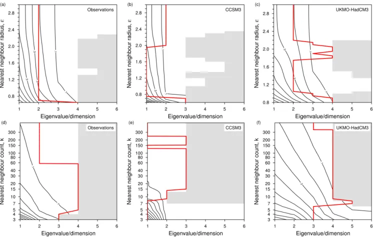
The leading modes of variability in tropical Pacific SSTs are the annual cycle and ENSO, and we expect Isomap to pick these out. As in the case of the Swiss roll data, it is useful to examine the sensitivity of Isomap results to varia-tions in the ε or k neighbourhood size parameters. Figure 7 displays Isomap sensitivity plots for observational SST data (Figs. 7a and 7d) and two selected models (Figs. 7b, 7c, 7e and 7f). Compared to the Swiss roll results (Fig. 6), the eigenvalue spectra and corresponding dimensionality es-timates for the SST data show more variation with Isomap neighbourhood size. The ranges of k and ε used in Fig. 7 are selected to correspond as far as possible, but it is difficult to relate results for any particular value of k to those for any particular value of ε or vice versa because of the variability in distances between data points. One common feature in the
ε-Isomap plots in Fig. 7 is that the regions of negative
eigen-values in the Isomap spectra disappear as the neighbourhood size increases. This reflects the equivalence of Isomap with a large neighbourhood size to PCA under suitable conditions of data normalisation: in the limit of infinite neighbourhood size, the geodesic distance approximation used in Isomap collapses to the use of the original Euclidean distances be-tween the data points, so is equivalent to PCA. The same ef-fect would also be seen in the k-Isomap results for k≈1000, the number of data points used.
Despite the high embedding dimension of the data (essen-tially the number of non-land points in the study region, m in Table 1), the dimensionality estimates inferred from Isomap in Fig. 7 are rather low. This is true for all models exam-ined and for the observational data. Table 2 shows the range of dimensionality estimates inferred for each dataset. For raw SSTs, across all datasets the dimensionality estimates range from 1 to a maximum of about 5. The eigenvalue spec-tra here converge rapidly because the leading modes of vari-ability are overwhelmingly larger in amplitude than the other modes. The coherent variation of SST patterns in the tropi-cal Pacific can easily be represented by a small set of modes. The convergence of the Isomap eigenvalue spectra is rather quicker than the convergence of eigenvalue spectra for PCA performed in a comparable setting, i.e. using raw SST data rather than SST anomalies, as shown in G´amez et al. (2004). This quicker convergence can be ascribed to better represen-tation of the nonlinear ENSO variability by Isomap than by
Fig. 7. Isomap eigenvalue convergence and dimension estimates for tropical Pacific raw SSTs, from observations (a and d), and two models,
CCSM3 (b and e) and UKMO-HadCM3 (c and f). Black contours show MDS eigenvalue spectra normalised by the overall largest eigenvalue, as a function of eigenvalue number and neighbourhood radius ε (a–c) or nearest neighbour count k (d–f) (logarithmic axis). The grey areas indicate regions of the eigenvalue spectra that are not useful for dimensionality reduction because of the presence of negative eigenvalues. The thick red line shows the data dimensionality, estimated from the eigenvalue spectra.
PCA. The PC scatter plots shown earlier (Fig. 4) demonstrate that ENSO variability is probably not a linear Gaussian phe-nomenon, so this is expected.
The range of dimension estimates shown in Table 2 for SST observations (2–4) is what we would expect, including two dimensions to describe the periodic annual cycle and one or two for ENSO variability. Here, two degrees of freedom are expected for the annual cycle because of the geometry of manifolds that can be faithfully represented by Isomap. The globally isometric transformation used by Isomap permits it to represent only simple Euclidean coordinates and not pe-riodic coordinates, meaning that any pepe-riodic phenomenon requires at least two degrees of freedom. There is no equiva-lent to the “circular” bottleneck layer NLPCA procedure de-scribed in Hsieh (2004) that allows periodic coordinates to be extracted directly. For ENSO variability, as well as the leading degree of freedom usually represented by the NINO3 SST index, previous studies have identified a second degree of freedom, varying in quadrature with the first,
correspond-ing to changes in the equatorial Pacific warm water volume (Burgers, 1999; Kessler, 2002; McPhaden, 2003).
Some model results show lower dimensional behaviour than this, including CCSM3 and CGCM3.1 (both T47 and T63). In the case of CCSM3, the reason for this behaviour is seen in the NINO3 power spectra in Fig. 2. Here, the observational data show a broad peak in the ENSO power band (2–7 years). CCSM3, however, has a sharper peak at almost exactly 2 years, displaying a mode of variabil-ity rather different from observed ENSO variabilvariabil-ity. In the Isomap analysis, this biannual variability is aliased with the annual cycle, and no distinct ENSO variability is detected. The situation with the CGCM3.1 models is different. Here, the NINO3 power spectrum shows essentially no peak in the ENSO frequency band. It is not clear what is happening here, but it may be relevant that the equatorial SST climatology in both CGCM3.1 models is poor, showing little or no gradient across the Pacific basin (Fig. 1).
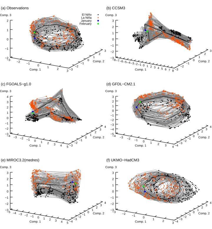
−3 −2 −1 0 1 2 3 −3 −2 −1 0 1 2 3 −2 −1 0 1 2 Comp. 1 Comp. 2 Comp. 3 (a) Observations El Niño La Niña January February −8−7−6−5 −4−3−2−1 0 1 2 3 4 5 6 7 8 −3 −2 −1 0 1 2 3 −3 −2 −1 0 1 2 3 Comp. 1 Comp. 2 Comp. 3 (b) CCSM3 −4 −3 −2 −1 0 1 2 3 4 5 −3 −2−1 0 1 2 3 4 −3 −2 −1 0 1 2 3 4 Comp. 1 Comp. 2 Comp. 3 (c) FGOALS−g1.0 −4 −3 −2 −1 0 1 2 3 4 −4 −3−2 −1 0 1 2 3 4 −5 −4 −3 −2 −1 0 1 2 3 Comp. 1 Comp. 2 Comp. 3 (d) GFDL−CM2.1 −5 −4 −3 −2 −1 0 1 2 3 4 5 −4 −3−2 −1 0 1 2 3 4 −3 −2 −1 0 1 2 3 Comp. 1 Comp. 2 Comp. 3 (e) MIROC3.2(medres) −3 −2 −1 0 1 2 3 −4 −3−2 −1 0 1 2 3 4 −3 −2 −1 0 1 2 3 Comp. 1 Comp. 2 Comp. 3 (f) UKMO−HadCM3
Fig. 8. Three-dimensional embeddings of Isomap raw SST results for observations (a) and selected models (b–f). Light grey lines join data
points representing adjacent months in the SST time series. The mean annual cycle is shown as a thicker line with January and February highlighted in blue and green respectively. Points are identified as El Ni˜no (black dots) or La Ni˜na (red triangles) events based on the corresponding NINO3 SST index time series for each dataset. For clarity, only 100 years of data is plotted here for each model.
Table 3. Correlation coefficients between NINO3 SST index and
warm water volume (WWV) and Isomap components from k-Isomap with k=7: for raw SSTs, the correlation between rotated Isomap component #3 and NINO3 and between rotated Isomap component #4 and WWV; for SST anomalies, the correlation be-tween Isomap component #1 and NINO3 and bebe-tween Isomap com-ponent #2 and WWV. Blank entries occur where the Isomap eigen-value spectrum in a particular case does not have enough positive eigenvalues to form an embedding of the required dimensionality.
Dataset Correlation Raw SST SST anomaly NINO3 WWV NINO3 WWV Observations 0.822 0.031 0.841 0.242 BCCR-BCM2.0 0.835 0.820 0.153 CCSM3 0.047 0.284 0.901 0.245 CGCM3.1(T47) 0.223 0.824 0.021 CGCM3.1(T63) 0.225 0.148 0.814 0.284 CNRM-CM3 0.824 0.225 0.776 0.228 CSIRO-Mk3.0 0.746 0.227 0.717 0.407 ECHO-G 0.907 0.681 0.935 0.646 FGOALS-g1.0 0.793 0.776 0.430 GFDL-CM2.0 0.857 0.435 GFDL-CM2.1 0.859 0.853 0.665 GISS-EH 0.652 0.665 0.116 INM-CM3.0 0.730 0.744 0.446 IPSL-CM4 0.844 0.852 n/aa MIROC3.2(hires) 0.236 0.171 0.686 0.070 MIROC3.2(medres) 0.646 0.785 0.087 MRI-CGCM2.3.2 0.861 0.909 0.511 UKMO-HadCM3 0.804 0.093 0.809 0.012 UKMO-HadGEM1 0.747 0.752 0.274
aOcean temperature data required to calculate warm water
vol-ume for IPSL-CM4 is not available.
Once we select a dimensionality for embedding of Isomap results, we can calculate reduced coordinates using Eq. (1). Here, we initially select an embedding dimensionality of three, both because this lies in the range derived from the Isomap eigenvalue spectra and because it is the highest di-mensionality of data we can easily visualise. Figure 8 illus-trates three-dimensional embeddings for SST observations and a selection of models. The Isomap results shown are all for k-Isomap with k=7. The plots show the data as a time series, with points adjacent in time connected by thin grey lines. The mean annual cycle is shown as a thicker line with January and February highlighted for orientation. Points identified as El Ni˜no or La Ni˜na events on the basis of the NINO3 SST index are picked out in colour. For clarity, only 100 years of the Isomap results are plotted in each case. Concentrating on the observations first, it can be seen that Isomap correctly identifies the annual cycle (represented by motion about the roughly cylindrical region occupied by the data points) and at least one other form of variability
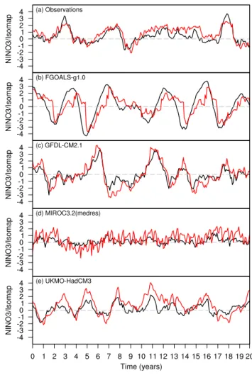
(repre-Fig. 9. Time series of NINO3 SST index (black) and rotated Isomap
component #3 (red) for observations (a) and selected models (b–e). An arbitrary 20 year slice of data is shown in each case.
sented by motion approximately in the direction of the axis of the cylindrical region). The clustering of El Ni˜no and La Ni˜na points indicates that this second mode of variability cresponds to ENSO and generally lies along the direction or-thogonal to the annual cycle in the embedding coordinates. Following G´amez et al. (2004), the role of the “axial” mode can be clarified by rotating the Isomap embedding to bring the mean annual cycle into the x-y coordinate plane. In this rotated coordinate system, variations in the z-direction record the “axial” variability in the original embedding coordinates (see Appendix for details of this rotation procedure). Time series plots of the rotated third Isomap component for ob-servations and four of the models selected here are shown in Fig. 9. The rotated Isomap component #3 time series are plotted in parallel with time series of the NINO3 SST in-dex, recording ENSO variability. For the observations, in Fig. 9a, it is clear that rotated Isomap component #3 quite accurately captures ENSO variability in the input SST data. In this case, Isomap has thus extracted the most important
modes of variability in tropical Pacific SSTs, the annual cycle and ENSO, starting from high-dimensional input data. We can also go further and attempt to extract the second degree of freedom in ENSO variability, usually identified with the equatorial Pacific WWV (Kessler, 2002; McPhaden, 2003), by examining a four-dimensional embedding of the Isomap results. The same sort of rotation procedure can be applied to remove the influence of the annual cycle variability on both Isomap components #3 and #4 (see Appendix for details). Correlation coefficients between Isomap rotated component #3 and the NINO3 SST index and between Isomap rotated component #4 and WWV are shown in Table 3. For the ob-servational data, the NINO3 correlation is high, as would be expected from Fig. 9a, but the correlation between rotated Isomap component #4 and WWV is very low. It thus appears that rotated Isomap component #4 here does not capture this second degree of ENSO variability.
Although the fact that Isomap appears to capture the an-nual cycle variability and at least some aspects of ENSO variability is unsurprising, the data-driven nature of Isomap makes it useful for comparison of model results with ob-servations and for inter-model comparison. We apply the same three-dimensional embedding to selected model results in Figs. 8b–f. Results for a number of the models shown (GFDL-CM2.1, MIROC3.2(medres) and UKMO-HadCM3) are similar to observations, with a clear three-dimensional structure to the data embedding, cleanly picking out the an-nual cycle and ENSO, with distinct clustering of El Ni˜no and La Ni˜na events. For the other two models illustrated, CCSM3 and FGOALS-g1.0, the three-dimensional Isomap embed-ding reveals data manifolds of significantly different form to that of the observations. As noted earlier, for CCSM3 this is due to excessively regular interannual variability in tropical Pacific SSTs that appears to be aliased with the annual cy-cle. For FGOALS-g1.0, the situation appears to be similar. The FGOALS-g1.0 NINO3 power spectrum in Fig. 2 exhibits a narrow peak at a period of around 3.5 years, rather than a broad peak stretching across the 2–7 year ENSO power band. This narrowband signal is again likely to result in lower-dimensional behaviour in the Isomap results.
Time series of rotated Isomap component #3 alongside the NINO3 SST index are plotted for a smaller selection of mod-els in Figs. 9b–e. Two of these cases, GFDL-CM2.1 (Fig. 9c) and UKMO-HadCM3 (Fig. 9e), are models whose three-dimensional Isomap embeddings show similar structure to observations. This is reflected in the rotated Isomap compo-nent #3 time series, which show good correlation with the NINO3 SST index. A good correlation is also seen for the results for FGOALS-g1.0 (Fig. 9b), despite the apparent de-generacy of the 3-D Isomap embedding in Fig. 8c. Despite the visual discrepancy between the FGOALS-g1.0 embed-ding results and the observations, it appears that the Isomap algorithm is still able to disentangle the annual and ENSO variability in the modelled SST data. The other model illus-trated in Fig. 9 is MIROC3.2(medres) (Fig. 9d), which has
weaker ENSO variability, but still shows a reasonable corre-lation between rotated Isomap component #3 and the NINO3 SST index.
For models with strongly degenerate three-dimensional Isomap embeddings, such as CCSM3 (Fig. 8b) and CGCM3.1(T47), CGCM3.1(T63) and MIROC3.2(hires) (not shown), the rotated Isomap component #3 time series show little coherent variability, and certainly none that correlates with ENSO variability. Correlation coefficients between ro-tated Isomap component #3 and the NINO3 SST index are shown in Table 3 for all models along with observational data. The models showing good correlations are those mod-els for which the three-dimensional Isomap embedding dis-plays a similar structure to the observations, i.e. for which Isomap successfully extracts the annual cycle and an “or-thogonal” ENSO mode. As for the observations, we can also attempt to identify a second degree of freedom of ENSO variability by examining four-dimensional Isomap embed-dings. One problem here is that, for some of the models, the Isomap eigenvalue spectra do not have enough positive lead-ing eigenvalues to provide a four-dimensional embeddlead-ing – at least four positive leading eigenvalues are required. In the cases where a four-dimensional embedding of the Isomap re-sults is possible, we conduct the same four-dimensional rota-tion as for the observarota-tions, to remove the annual variability from both rotated Isomap components #3 and #4, and then calculate correlation coefficients between the rotated Isomap components and the NINO3 SST index and simulated WWV time series, calculated as described in Sect. 2. As for the observations, the correlations between rotated Isomap com-ponent #4 and WWV for the models are generally rather low. As noted at the beginning of this section, one reason for applying Isomap to raw SST data, as opposed to SST anoma-lies, was to determine the extent to which Isomap is able to identify the coupling between annual and ENSO variabil-ity in the tropical Pacific. Other, more direct, analyses of ENSO/annual cycle interactions reveal a strong influence of the magnitude of the annual cycle in the equatorial Pacific on ENSO variability (Guilyardi, 2006). On the basis of the re-sults presented here, it appears that our Isomap analysis does not provide very much insight into this question.
5.2 Analysis for SST anomalies
In climatological contexts, PCA is normally applied to cli-mate anomalies, i.e. to data from which the mean annual cycle has been removed. This was the case for the equato-rial Pacific SST EOFs shown in Sect. 3. We can also ap-ply Isomap to SST anomalies, thus providing results that are more directly comparable with the results of PCA than the raw SST Isomap analysis presented in the previous section. These results may also be slightly easier to interpret because rotation to remove the influence of the annual cycle is not required.