HAL Id: hal-00330155
https://hal.archives-ouvertes.fr/hal-00330155
Submitted on 29 Nov 2007
HAL is a multi-disciplinary open access
archive for the deposit and dissemination of
sci-entific research documents, whether they are
pub-lished or not. The documents may come from
teaching and research institutions in France or
abroad, or from public or private research centers.
L’archive ouverte pluridisciplinaire HAL, est
destinée au dépôt et à la diffusion de documents
scientifiques de niveau recherche, publiés ou non,
émanant des établissements d’enseignement et de
recherche français ou étrangers, des laboratoires
publics ou privés.
wave regions in the magnetopause boundary layer
G. Stenberg, T. Oscarsson, M. André, A. Vaivads, M. Backrud-Ivgren, Y.
Khotyaintsev, L. Rosenqvist, F. Sahraoui, N. Cornilleau-Wehrlin, A.
Fazakerley, et al.
To cite this version:
G. Stenberg, T. Oscarsson, M. André, A. Vaivads, M. Backrud-Ivgren, et al.. Internal structure and
spatial dimensions of whistler wave regions in the magnetopause boundary layer. Annales Geophysicae,
European Geosciences Union, 2007, 25 (11), pp.2439-2451. �hal-00330155�
www.ann-geophys.net/25/2439/2007/ © European Geosciences Union 2007
Annales
Geophysicae
Internal structure and spatial dimensions of whistler wave regions in
the magnetopause boundary layer
G. Stenberg1,2, T. Oscarsson1,†, M. André2, A. Vaivads2, M. Backrud-Ivgren2,3, Y. Khotyaintsev2, L. Rosenqvist2, F. Sahraoui4, N. Cornilleau-Wehrlin4, A. Fazakerley5, R. Lundin6, and P. M. E. Décréau7
1Department of Physics, Umeå University, Umeå, Sweden 2Swedish Institute of Space Physics, Uppsala, Sweden
3Division of Plasma Physics, Alfvén Laboratory, Royal Institute of Technology, Stockholm, Sweden 4CETP/UVSQ, Vélizy, France
5MSSL, University College, London, UK
6Swedish Institute of Space Physics, Kiruna, Sweden 7LPCE et Université d’Orléans, France
†deceased
Received: 20 May 2007 – Revised: 27 October 2007 – Accepted: 5 November 2007 – Published: 29 November 2007
Abstract. We use whistler waves observed close to the mag-netopause as an instrument to investigate the internal struc-ture of the magnetopause-magnetosheath boundary layer. We find that this region is characterized by tube-like structures with dimensions less than or comparable with an ion iner-tial length in the direction perpendicular to the ambient mag-netic field. The tubes are revealed as they constitute regions where whistler waves are generated and propagate. We be-lieve that the region containing tube-like structures extend several Earth radii along the magnetopause in the boundary layer. Within the presumed wave generating regions we find current structures moving at the whistler wave group velocity in the same direction as the waves.
Keywords. Magnetospheric physics (Magnetopause, cusp and boundary layers; Plasma waves and instabilities) – Space plasma physics (Wave-particle interactions)
1 Introduction
The magnetopause constitutes the outer frontier defense of the magnetosphere. The border is not completely closed but the entry of the solar wind energy is restricted and regu-lated by the so-called reconnection process (Dungey, 1961; Paschmann, 1979). Ever since the magnetopause first was suggested to exist (Chapman and Ferraro, 1931) and even more since the first in situ observations where made (e.g. Sonett et al., 1959), there has been a huge interest in reveal-ing its secrets. Numerous studies are devoted to describe,
an-Correspondence to: G. Stenberg
alyze and model the structure and dynamics of this complex boundary.
Lately small-scale structures have received increased at-tention. The reconnection sites (diffusion regions), where the ion and electron motions are decoupled and the conversion of magnetic energy to particle energy takes place, are the heart of reconnection. Today, computer simulations and spacecraft observations are beginning to resolve the fine-structure in-volved (e.g. Vaivads et al., 2004a; Onofri et al., 2004; Retinò et al., 2006 and Mozer, 2005). Multi-spacecraft missions, such as Cluster (Escoubet et al., 1997; Escoubet et al., 2001), offer the opportunity to resolve the spatial-temporal ambigu-ity associated with single spacecraft measurements and allow us to determine the scale lengths of spatial structures.
Fascinating micro-physics are not only restricted to the reconnection sites. Thin electron-scale layers presumably associated with the separatrices are reported far away from the diffusion regions (e.g. André et al., 2004; Vaivads et al., 2004b and Retinò et al., 2006). Stenberg et al. (2005) show that whistler mode waves observed in the boundary layer on the magnetospheric side of the magnetopause are generated in thin (electron-scale) sheets. Furthermore, they suggest that although the sheets of whistler waves are observed thousands of kilometers from the magnetopause, they are still directly related to the diffusion region. As an inherent property of the near-magnetopause region, the thin layers with whistler mode waves and other small-scale structures may be the key to understanding the larger scale phenomena. They may also provide means of monitoring the micro-physics at the recon-nection site at large distances.
Whistler-mode waves have been observed by a number of spacecraft in the outer parts of of the magnetosphere. Elec-tromagnetic waves in a broad frequency range are reported
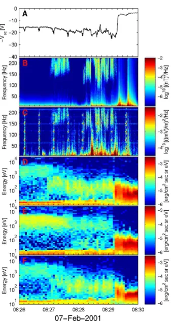
Fig. 1. The top panel shows the probe-to-spacecraft potential, which
can be used to estimate the density. The increase in density associ-ated with the magnetopause crossing in clearly seen at 06:29:10 UT. Frequency-time spectrograms of the electric and magnetic wave fields (from EFW and STAFF-SC) are presented in panels (B) and
(C). The artificial looking regularly spaced signatures in panel C
as well as the regularly spaced small dips in panel (A) are due to the active mode of the WHISPER instrument. Electron flux versus energy and time (from PEACE) for pitch angles 0◦, 90◦and 180◦ are displayed in the three bottom panels. During the two minutes of intense wave activity preceding the magnetopause crossing there is a mixture of cold (∼100 eV) magnetosheath electrons and hot (∼1 keV) magnetospheric electrons. All data are from Cluster 2.
from regions close to the magnetopause, in the outer cusp or in association with the bowshock by, e.g., Smith et al. (1967) (OGO-1); Olson et al. (1969) (OGO-3); Rodriguez and Gur-nett (1975) (Imp-6); Tsurutani and Smith (1977) (OGO-5);
Gurnett et al., 1979 (ISEE 1 and 2); LaBelle and Treumann (1988) (AMPTE/IRM); Zhang et al. (1998) (Geotail); Pick-ett et al. (1999) (Polar) and Maksimovic et al. (2001) (Clus-ter).
In this paper we examine the whistler wave-sheets reported by Stenberg et al. (2005) in closer detail. In particular, we determine the extension of these sheets in all three spatial di-mensions and we investigate the internal structure of the pre-sumed wave generating regions. We reveal that the whistler wave source regions are characterized by current structures moving at the whistler wave group velocity in the same direc-tion as the waves themselves. We estimate the size (perpen-dicular to the background magnetic field) of these structures to be about or less than 20 km, which corresponds to about 6 electron inertial lengths (c/ωpe). Simultaneously, our
anal-ysis suggests that the whistler wave emitting regions extend several Earth radii along the magnetic field lines.
2 Data
The four formation-flying Cluster spacecraft recorded the data used in this study. The satellite orbits are polar with a perigee of 4 Earth radii (RE) and an apogee of 19.6 RE.
Close to the magnetopause the satellites form almost a tetra-hedron. The spacecraft separation, which changes during the mission is 600 km and 100 km, respectively, for the two events considered below. The spacecraft are spin-stabilized with a spin period of 4 s and the instrumentation is identical on all four of them (Escoubet et al., 1997; Escoubet et al., 2001).
Data from six of the Cluster instruments are used in this study. The electric field experiment (EFW) (Gustafsson et al., 1997) and the search coil magnetometer (STAFF-SC) (Cornilleau-Wehrlin et al., 1997; Cornilleau-Wehrlin et al., 2003) provide time series wave field data. STAFF-SC measures three orthogonal magnetic wave field components, while EFW records two orthogonal electric field components in the satellite spin plane. Both instruments are run in burst mode, i.e., with a sampling rate of 450 samples/second, dur-ing both the events considered. The wave field signals are low pass filtered with a cutoff frequency of 180 Hz. We still choose to show data in all the spectrograms up to the Nyquist frequency (225 Hz), even if there is a small effect of the filter on both the wave amplitude and the phase above 180 Hz.
In addition, the STAFF Spectrum Analyser (STAFF-SA) gives electric and magnetic wave field spectral data in the frequency range 64 Hz–4 kHz. The WHISPER instrument (Décréau et al., 1997) captures electric wave field emissions in the frequency range 4–80 kHz, and provides a way of de-termining the plasma density from observations of the elec-tron plasma frequency.
The particle environment is investigated using the electron experiment PEACE (Johnstone et al., 1997) and the ion in-strument CIS/CODIF (Rème et al., 1997). Both inin-struments
can measure a 3-D distribution each spin period. CIS data are also used to estimate the plasma drift velocity.
We also use high resolution data (67.2 vectors/s) from the fluxgate magnetometer (FGM) (Balogh et al., 1997) to trans-form magnetic wave field data into a background magnetic field oriented coordinate system.
3 Boundary layer whistlers
An outbound magnetopause crossing is generally preceded by a passage through a boundary layer, presenting plasma populations of different origins (Eastman et al., 1976). The nature of the boundary layer depends on the latitude and the magnetic local time as well as solar wind and interplanetary magnetic field conditions (Haerendel et al., 1978).
The scene of action for the events to be discussed in this paper is a several thousand kilometer thick boundary layer characterized by a mixture of magnetospheric and magne-tosheath plasma. The thickness of the boundary layer is esti-mated from the time the spacecraft spend in the layer and the magnetopause velocity. The magnetopause passes the differ-ent spacecraft at differdiffer-ent times, which allow us to calculate its velocity to about 100 km/s. With a transit time through the boundary layer of about two minutes we arrive at a thickness of 12 000 km. In the case that the magnetopause is flapping back and forth during the two minutes, the thickness is over-estimated.
The study is based on two events; the first is introduced in Fig. 1. The observations are made by the Cluster spacecraft close to magnetic noon (13:24 MLT) at fairly high latitude (GSE: x=4.4 RE, y=5.7 RE, z=9.1 RE) on 7 February 2001.
The top panel presents the negative of the probe-to-spacecraft potential. This quantity varies as the density, where a less negative value (closer to zero in panel A) corresponds to a higher density (Pedersen et al., 2001). An outbound (magne-tosphere to magnetosheath) magnetopause crossing is seen as a sharp gradient at 06:29:10 UT, where the density suddenly increases.
The middle panels show the electric and magnetic frequency-time spectrograms revealing substantial electro-magnetic wave activity in the frequency range 100–200 Hz during two minutes prior to the crossing. The electron plasma frequency (from WHISPER) is 7.5 kHz and the back-ground magnetic field strength, B0, (from FGM) is about
20 nT (GSE: B0x=−14 nT, B0y=−14 nT, B0z=5 nT), giving
an electron gyrofrequency of 560 Hz. Assuming a proton-electron plasma the lower-hybrid frequency can be estimated to about 13 Hz. Hence, the observed electromagnetic waves are within the whistler mode frequency range, above the lower-hybrid frequency and below both the electron gyrofre-quency and the plasma fregyrofre-quency. We note that the emissions show a striped pattern, that is, they seem narrow in time and broad in frequency. The high-frequency part of the
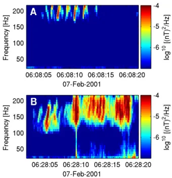
emis-Fig. 2. The near-magnetopause plasma features two different
fine-structured whistler wave emissions. Panel (A) shows chorus ele-ments observed in an environment of hot magnetospheric plasma only. The striped whistlers in panel (B) are recorded in the bound-ary layer just inside the magnetopause, where both magnetospheric and colder magnetosheath plasma is present. The data are from STAFF-SC on Cluster 2.
sions are not captured by the time series wave field data, but STAFF-SA shows that the emissions extend up to 400 Hz.
The bottom panels expose the characteristics of the bound-ary layer: hot (∼1 keV) magnetospheric electrons mixed with colder (∼100 eV) electrons originating from the mag-netosheath. The three panels display electron flux versus en-ergy and time for the pitch angles 0◦, 90◦and 180◦.
The second event we consider is an outbound magne-topause crossing, recorded on 2 March 2002. This event is extensively presented in Stenberg et al. (2005), and at first sight very similar to the event just discussed; waves in the whistler-mode frequency range are detected within a bound-ary region on the magnetospheric side of the magnetopause boundary. The particle data reveal a mixture of magneto-spheric and magnetosheath plasma. The reader is referred to Stenberg et al. (2005) for details and figures corresponding to Fig. 1.
4 Comparing boundary layer whistlers and chorus
Approaching the magnetopause we observe a change not only in the the particle distributions but also in the character of the wave emissions. The structure of the waves reveal the entry into the boundary layer. For example, fine-structured whistler waves are intermittently observed for at least half
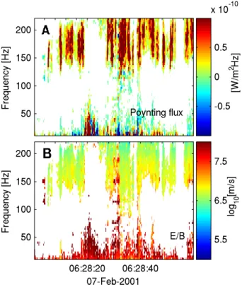
Fig. 3. Panel (A) presents the computed parallel Poynting flux. The
whistler mode waves (>100 Hz) all propagate parallel to the ambi-ent field. Panel (B) shows E/B, which is an estimate of the phase velocity. A phase velocity of about 107m/s corresponds to a wave-length of 100 km at 100 Hz. EFW and STAFF-SC data from Cluster 2 are used.
an hour preceding the magnetopause crossing on 7 February 2001, this is, long before the spacecraft enter the boundary layer. Panel A in Fig. 2 presents an example of such whistler mode waves detected before the Cluster spacecraft encounter the boundary layer. Although close to the Nyquist frequency at 225 Hz, the fine-structure of the emission is evident. We believe that these waves are chorus (e.g. Burtis and Helli-well, 1976) generated either close to the equatorial plane or in magnetic field minima at higher latitudes (Tsurutani and Smith, 1977). Chorus waves propagate along the magnetic field lines and can sometimes be reflected at lower altitudes and travel back toward the region of generation (Parrot et al., 2004).
The structure of the chorus emissions should be compared with that of the whistler emissions displayed in panel B. While the chorus emission is observed on closed field lines well inside the magnetosphere, the latter whistlers are ob-served in the boundary layer just inside the magnetopause. The boundary layer whistlers differ from the chorus emis-sions in several ways. While the chorus waves appear as emissions well separated and almost regularly spaced in time, the boundary layer whistlers are more irregular. Also, chorus emissions always show time dispersion, either as
risers (lowest frequencies recorded first, higher frequencies later) or fallers (the other way around). Although not very clearly seen, the strongest chorus elements in panel A are risers. The boundary layer whistlers, on the other hand, may show time dispersion (e.g., at 06:28:05 UT) but are most of-ten non-dispersive (e.g., at 06:28:10 UT). Another outstand-ing feature of the boundary layer whistlers is the extremely narrow-in-time but broad-banded feature extending all the way from the lowest frequencies up to the main whistler emission above 100 Hz. This feature, which is nicely illus-trated in panel B at 06:28:10 UT, plays a key role in this paper and we will return to this later.
We conclude that two types of fine-structured whistlers in the same frequency range are present in the near-magnetopause region. Chorus emissions are observed on field lines with magnetospheric plasma only, while the boundary layer houses whistlers showing a slightly striped pattern in the spectrogram. The remaining sections of this paper are devoted to the latter type.
5 Wave properties and generation regions
We begin our exploration of the boundary layer whistler mode waves by taking a closer look at the emissions asso-ciated with the magnetopause crossing at 7 February 2001 (Fig. 1). Based on the electromagnetic nature and the fre-quency range in which the waves are observed, we have already concluded that the observed emissions are whistler mode waves. A hodogram (not shown) confirms the ex-pected right-handed polarization and a Poynting flux calcu-lation (Fig. 3, panel A) shows that the whistlers propagate parallel to the background magnetic field. Panel B in Fig. 3 presents an estimate of the whistler wave phase velocity pro-vided by the ratio E/B, yielding ≈107m/s. At 100 Hz this corresponds to a wavelength of 100 km. We note that a cor-responding analysis for the March 2-event is performed in Stenberg et al. (2005), where the parallel wavelength is found to be about 50–200 km at 100 Hz. In that case the whistler waves instead propagates anti-parallel to the ambient mag-netic field.
A feature of boundary layer whistlers, already mentioned in Sect. 4, is occasionally occurring broadbanded signatures extending to very low frequencies. One such case is ev-ident in Fig. 2, panel B. We focus on the single stripe at 06:28:10 UT associated with a clear low frequency signa-ture that extends (in frequency) all the way up to the whistler emission. An enlargement of this detail is shown in panel A of Fig. 4.
To understand this structure we examine the wave vector (k) direction by applying Means’ method (Means, 1972). We use a magnetic field oriented coordinate system with the z-axis along B0. The direction of k is specified by the polar
angle, θ , (the angle between k and B0) and the azimuthal
Fig. 4 (panel B) the polar angle versus time and frequency is presented. For clarity all time-frequency bins with a spec-tral density below 8×10⁻⁷nT2/Hz or a polar angle outside
the interval 0–90◦are removed. The analysis does not dis-tinguish between k and −k and we invoke the Poynting flux calculation (Fig. 3) to remove this ambiguity. We conclude that the waves propagate almost parallel to B0in a 30◦wide
cone.
In panel C the direction of the wave vector in the plane perpendicular to B0is plotted versus time and frequency. As
in the previous panel all time-frequency bins with a spectral density below 8×10⁻⁷nT2/Hz are removed for clarity. We see a clear shift of the wave vector direction in the middle of the wave emission coinciding with the signal at lower fre-quencies.
The local plasma drift, vdrift, is estimated from the
ion drift (CIS/CODIF) and E×B (EFW and FGM). The components in the magnetic field oriented coordinate sys-tem are vdrift,x=± 40 km/s, vdrift,y=100–200 km/s, vdrift,z=0–
150 km/s. The situation is outlined in Fig. 5. It depicts a small-scale structure, in which wave generation occurs, that passes the spacecraft. The waves are assumed to propagate out from the generation region. Hence, prior to the passing of such a region the spacecraft will observe waves approach-ing from one direction (blue arrows), while after the region has passed the waves would reach the spacecraft from the op-posite direction (yellow arrows). Thus, we interpret the ob-servations as a wave-generating spatial structure passing the spacecraft with the plasma drift velocity. We conclude that such a generation region is recognized by a shift in the wave vector azimuthal angle, but also by a simultaneous narrow (in time) low frequency emission. During the two-minute long wave emission there are additional examples of sudden and distinct changes in the azimuthal wave vector compo-nent, all coinciding with low frequency features. Thus, the low-frequency signatures appears to be markers of whistler wave generation and we will take a closer look at them in the next section. Equivalent shifts in the azimuthal angle coin-ciding with low-frequency waves are found also in the March 2-event (Stenberg et al., 2005).
It should also be mentioned that in both of the discussed events the WHISPER instrument record waves in a broad frequency range around the local electron plasma frequency (4–24 kHz). These high frequency waves occur at the same times as the whistler-mode waves and hence the propagation properties and/or generation/damping processes are probably related. Simultaneous whistlers and electron plasma oscilla-tions have previously been observed, e.g., in the solar wind by Kennel et al. (1980). The WHISPER observations from the March 2-event are discussed in Canu et al. (2006).
Fig. 4. Panel (A) shows a detail of the wave emission presented in
Fig. 2 (panel B). We note the low frequency signature marked with a circle. Panels B and C present the results from the Means’ analy-sis. The polar angle, θ is displayed in panel B. The wave propagate in a 30◦wide cone almost parallel to B0. The azimuthal angle, φ is
plotted versus time and frequency in the bottom panel. Coinciding with the low frequency signature, there is a shift in the azimuthal wave vector direction. We interpret this as a generation region pass-ing the spacecraft.
6 The low frequency signatures
As seen in Fig. 4 the region with low frequency waves is much smaller than the region where the whistler wave emis-sion (>100 Hz) is detected. In the presented spectrogram the size of the structure is just a few pixels wide and the actual width cannot be determined from there. Instead, we consider the original time series data. To easily identify the struc-ture we low pass filter the time series, removing frequencies above 50 Hz. Figure 6 presents the filtered time series of the three magnetic field components. It turns out that the broad-banded signature in the spectrogram is not a wave feature at all, but appears as a narrow gradient structure in the middle of the time interval shown. The amplitude of the structure is about 0.2 nT, which is same as the typical whistler-mode wave amplitude. No corresponding signature is seen in the electric wave field data (not shown). Investigating the other cases during two-minute-long emission, where a shift in the azimuthal component of the wave vector coincides with a
Waves Generation region =150 km/s =150 km/s B v B drift φ v y x drift
Fig. 5. A whistler wave structure containing a generation region
passes the spacecraft with the plasma drift velocity. The observed wave vector directions are illustrated by colored arrows, where the colors are the same as used in panel C in Fig. 4. The waves are assumed to propagate out of the generation region, with an angle between k and B0in the range 0–30◦. As the generation region pass
we record a sudden shift in the propagation direction in the plane perpendicular to B0. Note that we only indicate the perpendicular component of the plasma drift velocity.
.8 .9 06:28:10.0 −0.8 −0.6 −0.4 −0.2 0 0.2 Magnetic field [nT] 07−Feb−2001 x y z
Fig. 6. The time series from STAFF-SC on Cluster 2 is low pass filtered with the maximum frequency 50 Hz. The low fre-quency emission seen in the spectrogram (e.g. Fig. 4) now appear as gradient structures in the components of the magnetic field at 06:28:09.96 UT.
low-frequency signature, we find similar features: The time series data reveals not low frequency waves but instead mag-netic field structures. Unfortunately, we cannot find a case where we are convinced that the same singular structure is seen by two different spacecraft. Hence, we have no means of determining the temporal and spatial characteristics of the structures. Fortunately, the second event we consider turns out to be a source of further knowledge.
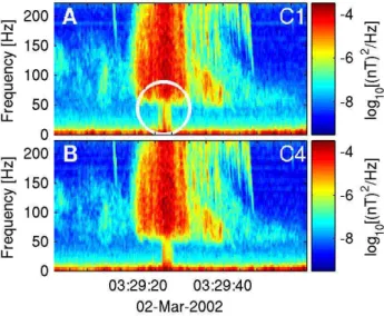
Fig. 7. Time-frequency spectrograms for spacecraft C1 and C4
observed in the boundary layer about 1.5 min before an outbound magnetopause crossing. The magnetic wave field is recorded by STAFF-SC. The waves with frequencies >50 Hz are whistler mode waves. In the middle of the two panels a low frequency signature is seen (indicated by a circle in panel A).
Figure 7 shows frequency-time spectrograms of the mag-netic field observed by Cluster 1 (C1) and Cluster 4 (C4) on 2 March 2002, prior to an outbound magnetopause crossing at 03:31 UT. All data is recorded in a boundary layer, where both magnetospheric and magnetosheath plasma are present. We note the wave activity at whistler mode wave frequencies (>50 Hz) but also a low-frequency signature (marked by a circle in panel A), that seems to be seen by both spacecraft. As in the previously shown cases this signature coincides with a clear shift in the azimuthal wave vector component (Stenberg et al., 2005).
Low-pass filtering the time series yields the result pre-sented in Fig. 8. The three magnetic wave field components are plotted versus time for the two spacecraft C1 and C4. The coordinate system used is background magnetic field ori-ented with the z-component along the ambient field. We see that there are several different magnetic structures present during the time interval shown. They are seen in all three field components and they all have about the same ampli-tude. In particular, we note that the parallel (z) component is no different from the perpendicular (x and y) components. Again, the amplitude of the structures is comparable to the whistler wave amplitude.
Although it is obvious that the same signatures truly are captured by both satellites, their appearance differ consider-ably between the spacecraft. Furthermore, there is a small time shift between the recordings, where C4 lags C1 with 0.01 s. It is worth mentioning that the sequence contain-ing this type of magnetic structures is actually much longer. It starts at 03:29:24.7 UT and lasts for 3 s. The magnetic
Fig. 8. Time series of the three magnetic wave field components
(STAFF-SC) observed by C1 (black) and C4 (red). The data are band pass filtered between 1–50 Hz. The coordinated system used is magnetic field oriented with the z-component along the ambient field.
structures shown in Fig. 8 are typical and the time span is chosen to make the time shift between the spacecraft clearly visible.
To sort out the situation we notice that the two space-craft are almost on the same magnetic field line, separated by 100 km along the field. Hence, for a signal to reach C4 0.01 seconds after being detected on C1 it must move with the speed 107m/s anti-parallel to the field. This velocity is the group velocity of the whistler waves. We can then estimate the parallel size of magnetic step-like structures in Fig. 8. As-suming a typical jump takes about 0.01 s the corresponding size is 100 km, which is about an ion inertial length (c/ωpi).
The perpendicular size is likely to be of the order of the spacecraft separation, noting that the observations made by C1 and C4 are considerably different. The satellite separation perpendicular to the background magnetic field is 30 km.
We argue that the discovered magnetic step-like features are current structures moving together with the whistler waves at the group velocity and with a perpendicular size of
Fig. 9. Time-frequency spectrograms (STAFF-SC) for the four spacecraft. The horizontal lines mark regions where two satellites appear to record the same emissions.
30–100 km (less than an ion inertial length). These features are commonly observed within or close to the regions where the whistler mode waves appear to be generated.
7 Size matters
Returning to an overview of the whistler wave emission recorded on 7 February 2001 (Fig. 9), we proceed with esti-mating the three-dimensional size of the singular stripe-like whistler emissions. Figure 9 shows about 70 s of data. All four Cluster spacecraft observe whistler waves while cross-ing the boundary layer. A comparison between the emissions
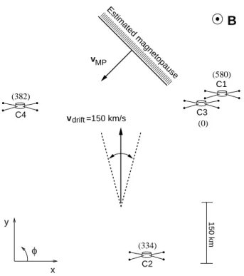
150 km =150 km/s (0) (580) (334) (382) vMP φ y x drift v
B
C4 C3 C2 C1 Estimated magnetopauseFig. 10. The location of the Cluster spacecraft in the magnetic field
reference frame. The background magnetic field is directed out of the figure. An estimate of the magnetopause normal is shown. Il-lustrated is also the plasma drift, which is varying during the time interval analyzed. The numbers in parenthesis are the spacecraft distances (in km) in the direction parallel to B0with respect to the
reference Cluster 3.
seen by the different satellites allows us to add new pieces of information.
We realize that although all panels show the similar striped wave emission character, it is not easy to identify the same structures on the different spacecraft. We concentrate on a few time intervals, where such an identification is possible.
Comparing Cluster 2 (C2) and Cluster 3 (C3) we find a sequence in the middle of the time interval shown, where the spacecraft appear to capture the same wave emissions. The roughly 12 s long sequence is indicated by a horizontal white line in the two panels. There is a timeshift of about two seconds between the observations, where C2 detects the emissions before C3 does. This time delay fits nicely with the estimates of the plasma drift velocity and the location of the spacecraft.
Figure 10 presents the situation in the magnetic field ori-ented system used throughout the paper. The location of the four spacecraft is indicated as well as an estimate of the mag-netopause normal. Note though that all spacecraft are well on the magnetospheric side of the boundary. The plasma drift is varying as indicated in Fig. 10 but is mainly in the y-direction. With a perpendicular distance of 400 km be-tween C2 and C3 and an averaged plasma drift during the
time period of 150 km/s, we would expect a time difference of a few seconds between the observations if the structures are fixed with respect to the plasma. In addition, each indi-vidual stripe seems to be about one second long in the time-frequency spectrograms. That means their physical size is about 150 km. The typical width of a stripe can be estimated from Figs. 2 and 4. Hence, we conclude that the whistler wave emissions are 150 km wide, spatial regions moving with the background plasma. Furthermore, we conclude that the structures are preserved for at least a couple of seconds.
It should also be noted that neither C1 nor C4 observe these whistler wave structures. Thus, these wave regions move with the plasma from C2 to C3 without hitting the other two satellites. Hence, the dimension perpendicular to the drift velocity in the plane shown in Fig. 10 must be smaller than the spacecraft separation (≈600 km).
Next, we compare spacecraft C1 and C3. As seen from Fig. 10, these two satellites are close to each other in the plane perpendicular to B0. C1 and C3 detect the same
emis-sions on two occaemis-sions, one at the beginning and one towards the end of the time interval shown in Fig. 9. These regions are marked with horizontal light blue lines in panels A and C. It is difficult to observe any time shift at all between the ob-servations in either of the cases. This is not surprising con-sidering the short distance between the spacecraft in the di-rection perpendicular to B0. With a plasma drift of 150 km/s
the time difference would never exceed fractions of a sec-ond. Along B0the waves themselves propagate at a speed
of 10 000 km/s and two satellites on the same field line sep-arated by no more than 600 km will record the waves almost simultaneously. The observation confirms our conclusions from comparing C2 and C3.
We emphasize that we determine the width of the whistler emission structure in the direction parallel to vdrift, but we
have no means to directly measure the size perpendicular to the drift velocity. From the C2/C3 comparison can only say that it is less than 600 km. However, we also note that all the striped whistler wave emissions seem to have about the same size in the spectrogram. This implies that the structures are either almost symmetric in the plane perpendicular to B0,
or they are oriented so that the minor/major axis is always parallel to the drift velocity. While some kind of ordering with respect to vdriftis not impossible, we believe that the
effect is mostly due to the fact that the structures are compa-rable in size in both directions perpendicular to B0. Figure 5
represents a compromise with one perpendicular dimension slightly larger and aligned perpendicular to the drift velocity. The generation of the whistler mode waves probably takes place in smaller regions in the middle of the observed emis-sions, where also the current structures discussed in the pre-vious section are found.
In summary, we believe that the regions in which the whistler waves are observed, as well as the presumably smaller generation regions within them, are tube-like struc-tures. The regions, where waves are observed have a
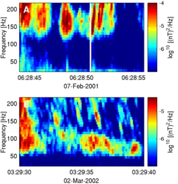
Fig. 11. Examples of risers and fallers. Panel (A) is an example of
risers found by Cluster 2 in the boundary layer on 7 February 2001. The example in panel (B) is taken from a magnetopause crossing on 2 March 2002. The presented whistler waves are observed by Cluster 1 in a boundary layer with the same mix of high and low energy electrons. Several fallers are clearly visible. In both panels data from STAFF-SC is used.
perpendicular size parallel to the drift velocity of about 100– 200 km. The size perpendicular to drift velocity is most prob-ably comparable to, but definitely less than, 600 km.
8 The third dimension: risers and fallers
The extension of the whistler mode wave stripes along the field lines still has to be estimated. This section will be de-voted to that issue, and we will focus on the dispersive ele-ments observed in the wave emission.
The accepted view of chorus (cf. Sect. 4) is that the rising and/or falling tones are created by the particular mechanism generating the waves (Helliwell, 1967). This is in contrast to lightning-generated whistler waves in the ionosphere, where the observed time dispersion is due to a propagation effect, (e.g., Storey, 1953). Boundary layer whistlers are observed not far from regions of chorus and they sometimes show a clear time dispersion. This is shown already in Fig. 2. An-other example of risers taken from the same event is dis-played in Fig. 11 (panel A). Whistlers in the boundary layer may also appear as fallers. Panel B in Fig. 11 shows such a case taken from the magnetopause crossing on 2 March 2002. It is not clear what causes the time dispersion of boundary layer whistlers, propagation effects or a chorus-like
gener-0 50 100 150 200 2 4 6 8x 10 6 Frequency [Hz]
Parallel phase velocity [m/s]
0 50 100 150 2000.5 1 1.5 x 10⁷
Parallel group velocity [m/s]
Fallers, 2002−03−02
B
v ph v gz 0 50 100 150 200 5 10 15x 10 6 Frequency [Hz]Parallel phase velocity [m/s]
0 50 100 150 200
1.3 1.4 x 10⁷
Parallel group velocity [m/s]
Risers, 2001−02−07
A
v ph v gzFig. 12. The dashed lines show the parallel group velocity, vgz,
ver-sus frequency for two cases. Panel (A) presents a case where risers can be formed above 100 Hz. In panel (B) the group velocity in-creases with frequency in the interval 0–200 Hz, which would give rise to fallers. The phase velocity, vph, (solid lines) increases with
frequency for both cases.
ation mechanism. However, the boundary layer whistlers observed on 7 February 2001 show a large number of sud-den changes of the azimuthal component of the wave vector indicating that the satellites pass through several generation regions. In all these cases the whistler wave elements are non-dispersive. This speaks in favor of explaining the time dispersion of boundary layer whistlers as a propagation ef-fect.
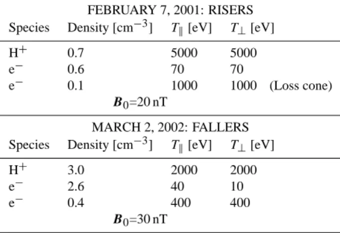
To investigate if it is possible that the risers and fallers observed in the boundary layer are due to propagation ef-fects we investigate the wave properties using the dispersion solver WHAMP (Rönnmark, 1982). The plasmas observed in the two events shown in Fig. 11 are modelled as presented in Table 1. For the risers’ event we use a plasma density of 0.7 cm−3and a background magnetic field of 20 nT. The ions are isotropic 5 keV protons, the magnetosheath electrons are regarded isotropic with a thermal energy of 70 eV, and the hot magnetospheric electrons are modelled using a 1 keV loss-cone distribution. The model describing the fallers event is discussed in Stenberg et al. (2005). In that case the total den-sity is higher and there is no loss cone distribution. Instead, the magnetosheath electrons have a temperature anisotropy.
Figure 12 shows that both risers and fallers are possible to explain using these plasma models. Panel A shows the attempt to model the situation in the major event discussed
Table 1. The plasma models used to recreate risers and fallers. All
components are assumed to be Maxwellians, in one case including a loss-cone, as indicated in the table. The models are based on PEACE and CIS observations. The model for the 2 March 2002 event is previously used in Stenberg et al. (2005).
FEBRUARY 7, 2001: RISERS Species Density [cm−3] Tk[eV] T⊥[eV]
H+ 0.7 5000 5000
e− 0.6 70 70
e− 0.1 1000 1000 (Loss cone)
B0=20 nT
MARCH 2, 2002: FALLERS Species Density [cm−3] Tk[eV] T⊥[eV]
H+ 3.0 2000 2000
e− 2.6 40 10
e− 0.4 400 400
B0=30 nT
in this paper (7 February 2001). Here the group velocity de-creases with frequency above 100 Hz, producing risers in this frequency range. Lower frequencies propagate faster and ar-rive a head of the higher frequencies. In panel B both the group and phase velocities increase with frequency in the interval 0–200 Hz. Parallel propagating whistlers would in such a plasma evolve into fallers as the high frequencies travel faster.
More work is required to fully understand the dependence of the wave properties on different parameters in the mod-els. Our aim is merely to show that both risers and fallers are possible outcomes of realistic plasma models. The brief investigation show that the behavior of the group velocity is sensitive to the relative temperatures of the two electron com-ponents as well as to the width and depth of any loss-cone.
Viewed as a propagation effect, the observed time disper-sion is consistent with a picture where the whistler emisdisper-sions extend great distances along the magnetopause. For instance, consider the riser in panel A of Fig. 11, where the time dif-ference between waves at 100 and 200 Hz is about a quarter of a second. Furthermore, assume that the group velocities at 100 Hz (v100) and 200 Hz (v200) are given by the the
an-alytical results presented in Fig. 12. Then, to produce the observed time difference the wave must travel a distance, s, given by s/v200−s/v100=0.25 s. With v200=1.38×10⁷ m/s
and v100=1.44×10⁷m/s, s=12 RE. The numerical result
should not be regarded an exact value, but serve as an indi-cation of that the whistler wave emission regions may extend for long distances along the field lines.
9 The global picture
The whistler mode waves occur on field lines with a mix-ture of magnetospheric and magnetosheath plasma. Hence, these are, or have recently been, open field lines in order to allow inflow of magnetosheath plasma. Moreover, Sten-berg et al. (2005) suggests that the generation of the waves is due to an electron anisotropy, resulting from connecting magnetospheric and magnetosheath field through the mag-netopause, i.e., magnetic reconnection. This result agrees also with Vaivads et al. (2007). However, for both the events considered in this paper a northward interplanetary magnetic field (IMF) is observed. We would therefore expect the ma-jor reconnection X-line to be located tailward of the cusp, where the IMF and the magnetospheric field lines are anti-parallel. The Cluster spacecraft cross the magnetopause at high latitude sunward of the cusp and should not record any signs of this process. Neither do we observe any clear rota-tion of the magnetic field in the magnetopause plane, when the Cluster spacecraft pass this boundary minutes after the wave emission encounters. Hence, we can not provide any strong evidence of reconnection southward of the cusp. If such active processes exist at this time, our results suggests they are probably local, patchy and/or intermittent.
10 Discussion
In a previous paper (Stenberg et al., 2005) we suggest that the whistler waves just inside the magnetopause are generated in thin sheets. Now we are inclined to believe that whistler waves are generated and propagate in tube-like, perhaps even cylindrically symmetric, structures. The generation is lo-cated in the center of the tubes. It is not the first time tube-like structures have been found in this region of space. Exam-ples of such spatial structures are discussed in, e.g., Rezeau et al. (1993), Alexandrova et al. (2004) and Alexandrova et al. (2006), who study low-frequency Alfvénic activity at the magnetopause and in the magnetosheath respectively.
This study presents evidence of a large amount of tightly packed wave generating tubes in the magnetopause bound-ary layer. Moreover, the apparent mix of locally generated waves and waves that have propagated substantial distances suggests that a large region of the boundary layer is char-acterized by such small-scale structures. In Stenberg et al. (2005) it is argued that a whistler generation region pro-vide a direct link to the reconnection diffusion region. The magnetospheric electrons are found to disappear at the same time as the whistlers are observed. From this it is argued that the whistlers are observed on field lines directly con-nected to a reconnection region, thereby allowing the mag-netospheric electrons to escape. The duration of a single generation region in the present paper is too short to allow us to study the electrons in such detail. However, the event is in other respects very similar to that studied in Stenberg et al.
(2005). Hence, a speculation is that also in the present case the whistlers are observed on field lines directly connected to diffusion regions at the magnetopause. In that case, the tube-like emission structures found indicate a patchy and/or intermittent reconnection geometry. We note, however, that there are no global signs of reconnection processes sunward of the cusp. Bursty whistler-mode waves observed by the Po-lar spacecraft in the outer cusp have also been suggested to originate from a diffusion region (Pickett, et al., 2001).
Another interesting question is the small perpendicular size of the whistler wave elements. Observations as well as simulations show that magnetic field and density perturba-tions often correlate with whistler mode activity, (Moullard, 2002; Eliasson and Shukla, 2005a). Enhancements or cav-ities duct whistler waves along the ambient magnetic field. In our case we do not observe any field or density fluctua-tions correlating with the individual wave elements but the situation, especially for the February 7-event, is complicated with overlapping wave regions. Thus, we cannot rule out this explanation.
We also lack the full explanation of the step-like magnetic field structures observed within the waves. They are ob-served in or close to regions where the waves are generated and where the waves are most intense, although the intensity is not extraordinary. It is known that whistler mode waves can be subject to linear or non-linear self-focusing, (Elias-son and Shukla, 2005b). One suggestion is then that such a process is responsible for the observed phenomena.
11 Summary of conclusions
The focus of this paper is whistler mode waves observed close to the magnetopause in the boundary layer on the mag-netospheric side of the boundary. In a time-frequency spec-trogram the waves appear as stripes, narrow in time and broader in frequency. With the help of the four-spacecraft mission Cluster we are able to determine both the three-dimensional size of the wave emissions and their internal structure. The main conclusions are summarized below:
– The whistler mode waves are observed in tube-like structures in space, extending a long way along the field lines (see below) but limited to about an ion inertial length (or less) in the perpendicular direction.
– Some of the whistler wave elements are non-dispersive. An investigation of the wave vector direction reveals a sudden and distinct change of the azimuthal component in the middle of such emission elements. We argue that these are regions, where waves are generated. As a con-sequence, plasma of the boundary layer is organized in tubes, which favor whistler wave generation.
– Within the presumed locally generated whistler waves we detect ion-scale current structures, that propagate
with the whistler wave group velocity in the same di-rection as the waves. The amplitude of the current struc-tures is comparable to the whistler wave amplitude. – Other whistler emission elements are clearly dispersive.
They manifest themselves as risers or as fallers. Using simple plasma models we conclude that it is possible to explain both cases as a propagation effect. This allows us to estimate the extension of the emissions along the ambient field. We find that the whistler waves propagate at least 10 RE.
– The large amount of detected generation regions (iden-tified as non-dispersive emission elements) indicates a high density of the tube-like structures in the plasma. Referring to Stenberg et al. (2005), where a whistler generation region is believed to couple directly to the re-connection site, we speculate that the observed pattern of tube-like regions reflects ongoing intermittent and/or patchy reconnection.
Acknowledgements. We are grateful to A. Balogh and S. Buchert
for supplying FGM data to this study and for useful discussions. Topical Editor F. D’Andrea thanks two anonymous referees for their help in evaluating this paper.
References
André, M., Vaivads, A., Buchert, S. C., et al.: Thin electron-scale layers at the magnetopause, Geophys. Res. Lett., 31, L03803, doi:10.1029/2003GL018137, 2004.
Alexandrova, O., Mangeney, A., Maksimovic, M., et al.: Cluster observations of finite amplitude Alfvén waves and small-scale magnetic filaments downstream of a qusi-perpendicular shock, J. Geophys. Res., 109, A05207, doi:10.1029/2003JA010056, 2004. Alexandrova, O., Mangeney, A., Maksimovic, M., et al.: Alfvén vortex filaments observed in magnetosheath downstream of a quasi-perpendicular bow shock, J. Geophys. Res.,111, A10, 10.1029/2006JA011934, 2006.
Balogh, A., Dunlop, M. W., Cowley, S. W. H., et al.: The Cluster Magnetic Field Investigation, Space Sci. Rev., 79, 65–91, 1997. Burtis, W. J. and Helliwell, R. A.: Magnetospheric chorus:
Occur-rence patterns and normalized frequency, Planet. Space Sci., 24, 1007–1024, 1976.
Canu, P., Décréau, P., Escoffier, S., et al.: A search for electron scale structures close to the magnetopause, Cluster and Double Star Symposium, 5th Anniversity of Cluster in Space, ESA SP-598, European Space Agency, 2006.
Chapman S., and Ferraro, V. C. A.: A new theory of magnetic storms, Terrestr. Magn. Atmos. Elec., 36, 77–97, 171–186, 1931. Cornilleau-Wehrlin, N., Chauveau, P., Louis, S., et al.: The Clus-ter spatio-temporal analysis of field fluctuations (STAFF) exper-iment, Space Sci. Rev., 79, 107–136, 1997.
Cornilleau-Wehrlin, N., Chanteur, G., Perraut, S., et al.: First results obtained by the Cluster STAFF experiment, Ann. Geophys., 21, 437–456, 2003,
Décréau, P. M. E., Fergeau, P., Krannosels’kikh, M., et al.: WHIS-PER, a resonance sounder and wave analyser: Performance and perspectives for the Cluster mission, Space Sci. Rev., 79, 157– 193, 1997.
Dungey, J. W.: Interplanetary magnetic fields and the auroral zones, Phys. Rev. Lett., 6, 47–48, 1961.
Eastman, T. E., Hones, Jr., E., W., Bame, S. J., et al.: The magneto-spheric boundary layer: Site of plasma, momentum, and energy transfer from the magnetosheath into the magnetosphere, Geo-phys. Res. Lett., 3, 685–688, 1976.
Eliasson, B. and Shukla, P. K.: Three-dimensional dynamics of non-linear whistlers in plasmas, Phys. Lett. A, 348, 51–57, 2005a. Eliasson, B. and Shukla, P. K.: Linear self-focusing of whistlers in
plasmas, New Journal of Physics, 7(95), 1–10, 2005b.
Escoubet, C. P., Schmidt, R., and Goldstein, M.: Cluster – Science and Mission Overview, Space Sci. Rev., 79, 11–32, 1997. Escoubet, C. P., Fehringer, M., and Goldstein, M.: The Cluster
Mis-sion, Ann. Geophys., 19, 1197–1200, 2001, http://www.ann-geophys.net/19/1197/2001/.
Gurnett, D. A., Anderson, R. R., Tsurutani, B. T., et al.: Plasma Wave Turbulence at the Magnetopause: Observations From ISEE 1 and 2, J. Geophys. Res., 84, 7043–7058, 1979.
Gustafsson, G., Boström, R., Holback, B., et al.: The electric field and wave experiment for the Cluster mission, Space Sci. Rev., 79, 137–156, 1997.
Haerendel, G., Paschmann, G., Sckopke, N., et al.: The frontside boundary layer of the magnetosphere and the problem of recon-nection, J. Geophys. Res., 83, 3195–3216, 1978.
Helliwell, R. A.: A Theory of Discrete VLF Emissions from the Magnetosphere, J. Geophys. Res., 72, 4773–4790, 1967. LaBelle, J. and Treumann, R. A.: Plasma waves at the dayside
mag-netopause, Space Sci. Rev., 47, 175–202, 1988.
Johnstone, A. D., Alsop, C., Burge, S., et al.: PEACE: A plasma electron and current experiment, Space Sci. Rev., 79, 351–398, 1997.
Kennel, C. F., Scarf, F. L., Coroniti, F. V., et al.: Correlated Whistler and Electron Plasma Oscillation Bursts Detected on ISEE-3, Geophys. Res. Lett., 7, 129–132, 1980.
Maksimovic, M., Harvey, C. C., Santolík, O., et al.: Polarization and propagation of lion roars in the dusk side magnetosheath, Ann. Geophys., 19, 1429–1438, 2001,
http://www.ann-geophys.net/19/1429/2001/.
Means, J. D.: Use of the Three-Dimensional Covariance Matrix in Analyzing the Polarization Properties of Plane Waves, J. Geo-phys. Res., 77, 5551–5559, 1972.
Moullard, O., Masson, A., Laakso, H., et al.: Density modu-lated whistler mode emissions observed near the plasmapause, Geophys. Res. Lett., 29(20), 1975, doi:10.1029/2002GL015101, 2002.
Mozer, F. S.: Criteria for and statistics of electron diffusion re-gions associated with subsolar magnetic field reconnection, J. Geophys. Res., 110, A12222, doi:10.1029/2005JA011258, 2005. Olson J. V, Hozer, R. E., and Smith, E. J.: High-Frequency Mag-netic Fluctuations Associated with the Earth’s Bow Shock, J. Geophys. Res., 74, 4601–4617, 1969.
Onofri, M., Primavera, L., Malara, F., and Veltri P.: Three-dimensional simulations of magnetic reconnection in slab geom-etry, Phys. Plasmas, 11, 4837–4846, 2004.
Parrot, M., Santolík, O., Gurnett, D. A., et al.: Characteristics of
magnetospherically reflected chorus waves observed by CLUS-TER, Ann. Geophys., 22, 2597–2606, 2004,
http://www.ann-geophys.net/22/2597/2004/.
Paschmann, G.: Plasma acceleration at the Earth’s magnetopause: Evidence for reconnection, Nature, 282, 243–246, 1979. Pedersen, A., Décréau, P., Escoubet, C.-P., et al.: Four-point high
time resolution information on electron densities by the electric field experiment (EFW) on Cluster., Ann. Geophys., 19, 1483– 1489, 2001,
http://www.ann-geophys.net/19/1483/2001/.
Pickett, J. S., Menietti, J. D., Dowell, J. H., et al.: Polar spacecraft observations of the turbulant outer cusp/magnetopause boundary layer of Earth, Nonlinear Proc. Geophys., 6, 195–204, 1999. Pickett, J. S., Franz, J. R., Scudder, J. D., et al.: Plasma waves
observed in the cusp turbulent boundary layer: An analysis of high time resolution wave and particle measurements from the Polar spacecraft, J. Geophys. Res., 106, 19081–19099, 2001. Rème, H., Bosqued, J. A., Sauvaud, J. A., et al.: The Cluster Ion
Spectrometry (CIS) Experiment, Space Sci. Rev., 79, 303–350, 1997.
Retinò, A., Vaivads, A., André, M., et al.: The structure of the separatrix region close to a magnetic reconnection X-line: Cluster observations, Geophys. Res. Lett., 33, L06101, doi:10.1029/2005GL024650, 2006.
Rezeau, L., Roux, A., and Russell, C. T.: Characterization of Small-Scale Structures at the Magnetopause From ISEE Measurements, J. Geophys. Res., 98, 179–186, 1993.
Rodriguez, P. and Gurnett, D. A.: Electrostatic and Electromagnetic Turbulence Associated With the Earth’s Bow Shock, J. Geophys. Res., 80, 19–31, 1975.
Rönnmark, K.: WHAMP — Waves in Homogeneous Anisotropic Multicomponent Plasmas, KGI Report 179, Kiruna Geophysical Institute, 1982.
Smith E. J., Holzer, R. E., McLeod, M. G., et al.: Magnetic Noise in the Magnetosheath in the Frequency Range 3–300 Hz, J. Geo-phys. Res., 72, 4803–4813, 1967.
Sonett, C. P., Judge, D. L., and Kelso, J. M.: Evidence concerning instabilities of the distant geomagnetic field: Pioneer 1, J. Geo-phys. Res., 64, 941–943, 1959.
Stenberg, G., Oscarsson, T., André, M., et al.: Electron-scale sheets of whistlers close to the magnetopause, Ann. Geophys., 23, 3715–2725, 2005,
http://www.ann-geophys.net/23/3715/2005/.
Storey, L. R. O.: An investigation of whistling atmospherics, Philo-sophical transactions of the Royal Society of London, 246, 113– 141, 1953.
Tsurutani, B. T. and Smith, E. J.: Two Types of Magnetospheric ELF Chorus and Their Substorm Dependences, J. Geophys. Res., 82, 5112–5128, 1977.
Vaivads, A., André, M., Buchert, S. C., et al.: Cluster observations of lower hybrid turbulence within thin lay-ers at the magnetopause, Geophys. Res. Lett., 31, L03804, doi:10.1029/2003GL018142, 2004a.
Vaivads, A., Khotyaintsev, Y., André, M., et al.: Struc-ture of the magnetic reconnection diffusion region from four-spacecraft observations, Phys. Rev. Lett., 93, 105001, doi:10.1103/PhysRevLett.93.105001, 2004b.
Vaivads, A., Santòlik, O., Stenberg, G., André, M., Owen, C. J., Canu, P., and Dunlop, M.: The source of whistler emissions
at the dayside magnetopause, Geophys. Res. Lett., 34, L09106, doi:10.1029/2006GL029195, 2007.
Zhang Y., Matsumoto, H., and Kojima, H.: Bursts of whistler mode waves in the upstream of the bow shock: Geotail observations, J. Geophys. Res., 103, 20 529–20 540, 1998.