Intermittent Dynamics of Slow Drainage Experiments in Porous Media: Characterization Under Different Boundary Conditions

used for the calculation of temperature correction for a 7.6 lm thermocouple diameter: “U reference” a time resolved estimation based on PIV measurements in the location of the

In an effort to identify new mutations in the RYRl gene causing MHS, we have investigated the RYRl gene in unrelated MHS patients for the presence of new mutations by the SSCP

Additionally, it is noteworthy that the effect of T and P on slowing down the time scale of fast relaxation processes (β-relaxation and excess wing), although less strong than in

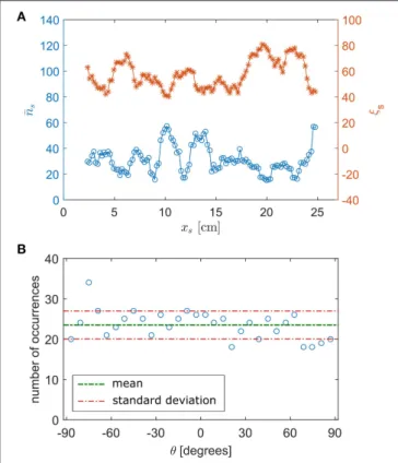
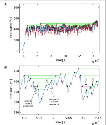
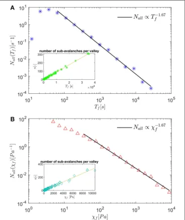
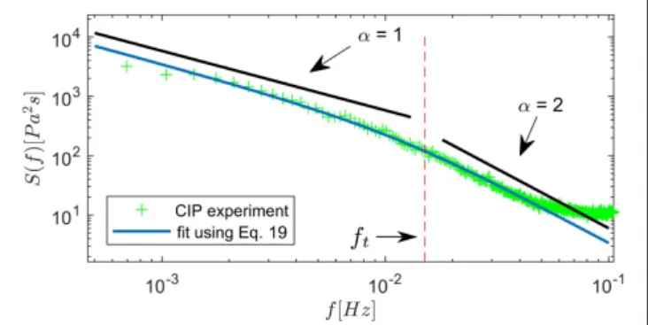
Assuming that experiments in larger systems can be conducted, the results should be useful to the identification of the correlation structure of the pore-space in porous media, based

magnetic field parallel to the ferroelectric b-axis figure 1 shows the relaxation rate for a free crystal and a crystal with shorted evaporated gold electrodes.. Near

Nous essayerons dans ce chapitre de donner les étapes de calculs essentielles pour évaluer la fréquence complexe et la bande passante d'une antenne micro-ruban

Comme dans le cas de la 5-fluoro cytosine, la structure cationisée la plus stable est celle pour laquelle le sodium est en interaction avec les atomes O2 et N3.. La

This indicates that a substorm does not always complete its current system by connecting the cross‐ tail current with both the northern and southern ionospheric currents (see