HAL Id: hal-00316267
https://hal.archives-ouvertes.fr/hal-00316267
Submitted on 1 Jan 1996
HAL is a multi-disciplinary open access
archive for the deposit and dissemination of sci-entific research documents, whether they are pub-lished or not. The documents may come from teaching and research institutions in France or abroad, or from public or private research centers.
L’archive ouverte pluridisciplinaire HAL, est destinée au dépôt et à la diffusion de documents scientifiques de niveau recherche, publiés ou non, émanant des établissements d’enseignement et de recherche français ou étrangers, des laboratoires publics ou privés.
Comparison of F-region electron density observations by
satellite radio tomography and incoherent scatter
methods
T. Nygrén, M. Markkanen, M. Lehtinen, E. D. Tereshchenko, B. Z.
Khudukon, O. V. Evstafiev, P. Pollari
To cite this version:
T. Nygrén, M. Markkanen, M. Lehtinen, E. D. Tereshchenko, B. Z. Khudukon, et al.. Comparison of F-region electron density observations by satellite radio tomography and incoherent scatter methods. Annales Geophysicae, European Geosciences Union, 1996, 14 (12), pp.1422-1428. �hal-00316267�
Ann. Geophysicae 14, 1422—1428 (1996) ( EGS — Springer-Verlag 1996
Comparison of F-region electron density observations by satellite radio
tomography and incoherent scatter methods
T. Nygre´n1, M. Markkanen2, M. Lehtinen2, E. D. Tereshchenko3, B. Z. Khudukon3, O. V. Evstafiev3, P. Pollari1
1 Department of Physical Sciences, University of Oulu, FIN-90570 Oulu 57, Finland 2 Geophysical Observatory, FIN-99600 Sodankyla¨, Finland
3 Polar Geophysical Institute, 15 Khalturina, 183023 Murmansk, Russia Received: 4 March 1996/Revised: 17 June 1996/Accepted: 18 June 1996
Abstract. In November 1995 a campaign of satellite radiotomography supported by the EISCAT incoherent scatter radar and several other instruments was arranged in Scandinavia. A chain of four satellite receivers extend-ing from the north of Norway to the south of Finland was installed approximately along a geomagnetic meridian. The receivers carried out difference Doppler measure-ments using signals from satellites flying along the chain. The EISCAT UHF radar was simultaneously operational with its beam swinging either in geomagnetic or in geo-graphic meridional plane. With this experimental set-up latitudinal scans of F-region electron density are obtained both from the radar observations and by tomographic inversion of the phase observations given by the difference Doppler experiment. This paper shows the first results of the campaign and compares the electron densities given by the two methods.
1 Introduction
Satellite radio tomography, a developing method for de-termining the ionospheric electron density, was originally suggested by Austen et al. (1986). A usual experimental set-up is to have a chain of ground-based receivers which carry out difference Doppler measurements using signals from navigational satellites passing the chain. Satellite-to-satellite set-ups are also possible. In difference Doppler measurements the observations consist of the phase differ-ence of coherent radio waves at two frequencies, e.g. 150 and 400 MHz, which is proportional to the integral of electron density (TEC, the total electron content) along the ray. Therefore, when the measurement is carried out along a great number of rays crossing each other at F-region altitudes, the method is suitable for tomographic
Correspondence to: T. Nygre´n
inversion. An ionospheric tomographic experiment can also, in principle, be carried out using Faraday rotation. The most common tomographic methods are based on ray approximation and are applicable as long as diffrac-tion effects are not important. They all belong to the class of ray tomography. When the ionosphere contains small-scale inhomogeneities, diffraction may be important. If the number of structures is small, they may be reconstructed by means of diffraction tomography, otherwise one has to be satisfied with their statistical properties which can be resolved by statistical tomography. Theory and examples of diffraction and statistical tomography are presented by Kunitsyn et al. (1994, 1995).
Numerous inversion methods and their modifications have been applied in satellite ray tomography. The most conventional ones are various iterative methods like ART, MART or SIRT (Censor, 1983; Austen et al., 1988; Raymund et al., 1990; Andreeva et al., 1992), as well as the maximum entropy method (Pakula et al., 1995; Fougere, 1995). In these algorithms the iteration begins from chosen start profiles and proceeds step by step until a given stop criterion is met. The choice of the model layer to be used as a starting point poses a central problem in these methods because the ultimate result more or less depends on it. Results obtained by these methods have been compared by Raymund (1995) and Vasicek and Kronschnabl (1995).
A second approach is to make the inversion in a single step with suitable matrix operations. Raymund et al. (1993, 1994) construct the ionosphere from a set of model base functions and carry out the tomographic inversion by a pseudoinversion of the matrix describing the map-ping from the function space to the measurement space. In this way the big inversion problem, with electron densities at given grid points as unknowns, is converted into a smaller one. A proper choice of the base functions, however, is a crucial point in this method.
In stochastic inversion the goal is to find the most probable values of electron density once the measurement is known. This approach also contains a single matrix operation and has been used in various forms by
Fremouw et al. (1992), Fehmers (1994) and Markkanen
et al. (1995). In big inversion problems some sort of
regu-larization is necessary in order to prevent too vigorous point-to-point oscillation of the result. One of the benefits of stochastic inversion is that it allows regularization to be used for feeding suitable a priori information to the inver-sion solver. A priori information is needed since, for geo-metrical reasons, the measurements contain very little information on the layer shape. Different ways of doing this have been presented by Markkanen et al. (1995) and Fehmers (1994). Although it may not be obvious at first sight, even the recursive algorithms use some a priori information. This is included in the applied start profile in a rather undetermined manner. In a stochastic inversion algorithm the role of a priori information can be dealt with in a much more controlled way.
In this paper results from a satellite tomography cam-paign arranged in Scandinavia in November 1995 are presented. The campaign was a continuation of a previous one arranged in January 1993 with practically the same instruments and receiver sites, described by Markkanen
et al. (1995). As before, the EISCAT incoherent scatter
radar was carrying out different types of measurements, but in this case an experiment with the radar beam swing-ing in the meridional plane was used part of the time. Therefore, F-region electron densities given by the two methods can be compared in a better way than in our earlier work. The first results of such comparisons are shown in this paper.
2 Experimental method and data analysis
The experimental set-up used in tomographic experiments in January 1993 was briefly described by Markkanen et al. (1995). Some development of the hardware and data col-lection software has been carried out since then, but the difference Doppler experiment is carried out essentially in the same way as before. One change is that the sampling frequency is now 50 Hz instead of the previous 200 Hz. The measurement also contains the signal amplitude, but this is not used in the present work.
In the November 1995 campaign the four receiver sites were essentially the same as in January 1993, only the southernmost site was shifted by a couple of tens of kilometres. The coordinates of the sites were measured using GPS receivers, so that they are now known more accurately than before. The receiver sites from north to south are: Tromsø (69.662°N, 18.940°E), Esrange (67.877°N, 21.064°E), Kokkola (63.837°N, 23.058°E) and Ka¨rko¨la¨ (60.584°N, 23.985°E). These points nearly lie on same line which almost coincides with a magnetic meridi-an (see the map in Markkmeridi-anen et al., 1995). The length of the chain is 1036 km and the site separations are 214, 458 and 364 km from north to south. The Russian satellites used in the experiment fly at an altitude of about 1000 km and their paths are very closely parallel to the receiver chain. Of course, a satellite only rarely flies just above the receivers, but the examples to be shown are selected from cases where the satellite path is not too far away from the receiver chain.
The inversion method used in the tomographic analysis is described by Markkanen et al. (1995). The vertical plane above the receiver chain is divided into a rectangular grid and electron density values at the grid points, together with the phase constants, are the unknown quantities to be determined. The grid elements are not necessarily of equal size, but larger ones can be used both at the highest and lowest altitudes as well as on the edges. Bilinear interpolation of electron density is used within each grid element. The algorithm is based on stochastic inversion and can be presented in terms of a few formally simple matrix operations involving the Fisher information matrix. A noteworthy property of the method is that the unknown phase constants have mathematically the same role as the unknown electron density values have. This is because each phase measurement is a linear combination of the unknown electron densities and a single unknown phase constant. Therefore, no separate method is needed for estimating the phase constants, but they are simply obtained simultaneously with the unknown electron dens-ities as a result of the mathematical inversion (see Mark-kanen et al., 1995).
In order to obtain stable solutions, the algorithm con-tains a regularization method which is based on a non-diagonal regularization matrix. The regularization matrix is constructed in such a way that it is mathematically equivalent to a measurement of electron density difference at neighbouring grid points both in horizontal and verti-cal direction. These differences are treated as Gaussian random variables with zero mean values, their variances can be adjusted by the user.
Regularization is used not only for obtaining stable solutions but also for a second purpose. The regulariza-tion variances are chosen in such a way that their values are large at F-region altitudes where the electron density is high and large steps from point to point are possible. Small variances are applied at low and high altitudes where only small electron density steps are expected. The procedure guides the solution more or less to a horizontal layer and roughly determines the layer thickness, al-though usually not the layer shape. This is quite essential since, in the absence of horizontal rays, the observations contain only little information on the layer thickness. Although the choice of the regularization does have some effect on the results, clear artifacts appear if the measure-ments and the regularization profile are not in a reason-able agreement with each other (Markkanen et al., 1995). The EISCAT experiment was arranged to contain a cycle of 57 beam directions southward of Tromsø in the geographic or geomagnetic meridional plane in order to cover the northern part of the region between the tomog-raphy sites. In the examples shown in the present paper the beam scan was in the geographic meridional plane. Three different correlator programmes were used for dif-ferent ranges of the elevation angle. The beam scan started from a nearly vertical direction above Tromsø with an elevation angle of 88.1° and ended at a low elevation angle of 16.1°. The elevation step varied between 2.8° and 0.4° in different parts of the beam swing. The radar modulation consisted of two parts which gave both a power profile in 250 range gates with a resolution varying from 1.5 to 3 km
Fig. 1. Comparison of F-region electron densities observed by the tomographic (top panel) and incoherent scatter (centre and bottom panel) methods. The time in the top panel indicates the start time of the satellite measurement and the time intervals in the other panels the start and stop times of the radar beam scan. The contour interval is
0.25 · 1011 m~3. The open dots on the horizontal axis show the satellite receiver sites and the tick marks on the top and right-hand side of the top panel indicate the grid used in the tomographic analysis. The radar electron densities are averages within the same grid
and a long-pulse spectrum measurement in 20 gates with a resolution varying roughly between 20 and 30 km. The measurement time for each beam direction was 10 s and the cycle time 20 min. This means that more than 50% of the total time was used for antenna motion.
A power profile measurement alone is not likely to give a correct electron density profile, because a proper tem-perature correction is not carried out (equal ion and electron temperatures are usually assumed) and the effect of Debye shielding is also neglected. Therefore, long-pulse data should actually be used. The long-pulse profile, how-ever, starts at such high altitudes that it covers the bot-tomside of the F layer poorly (for some beam directions the profile starts at 210—220 km). The long-pulse modula-tion will also produce somewhat too low electron densities at the layer peak. This is due to the spatial averaging effect caused by the long scattering volume. For these reasons the electron density was determined from power profile data taking results of long-pulse analysis for temperature
correction. The temperature profile ratio was interpolated to match the range resolution of the power profile and a model was used below the heights of the long-pulse experiment. Although its effect is usually very small, De-bye correction was also carried out.
2 Results
An example of F-region electron densities obtained by the tomographic and incoherent scatter methods is portrayed in Fig. 1. The top panel contains results from the tomo-graphic experiment and the middle and bottom panels radar observations from two successive beam scans. The same grey scale is used throughout the figure and, in addition, contours at intervals of 0.25 · 1011 m~3 are also drawn. The open dots on the horizontal axes, from left to right, indicate the geographic latitudes of the satellite receiver sites Ka¨rko¨la¨, Kokkola, Esrange and Tromsø.
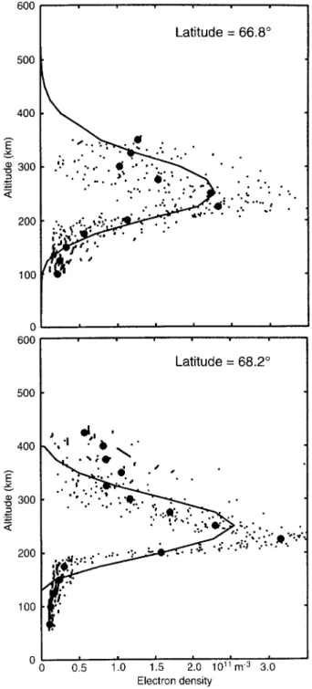
Fig. 2. Vertical electron density profiles at latitudes 66.8° and 68.2° from the measurements in Fig. 1. The continuous line indicates the tomographic observations, the large dots the averaged radar measurements from the second panel and the small dots the original radar measurements used in calculating the averages
The flight direction of the satellite is from north to south and each beam swing in radar measurements also starts from the north.
The result of tomographic inversion depends on the regularization variances, which should not conflict with the true difference Doppler measurements. If possible, the regularization profile should correspond roughly to the expected electron density profile. The best we can do is to use our a priori knowledge of the F-layer behaviour. Because this is a daytime observation, the altitude of the F-layer peak is most probably lower than at night and 250—280 km seems a reasonable guess (see e.g. Lanchester
et al., 1991). Therefore, a value of 250 km was taken for the
peak altitude of the regularization profile. The shape was chosen to be bi-Gaussian with widths of 100 and 150 km in the lower and upper parts, respectively. In this way the bottomside of the profile is steeper than the topside, and a reasonable estimate of the thickness of the F layer is obtained. It is important to notice that this choice by no means implies that the height profile of the inversion result would have the same shape or altitude as the regu-larization profile. From the fact that no clear artifacts appear in the results, we can conclude that the regulariz-ation is in reasonable agreement with the measurements. The grid in the tomographic inversion was selected to have a vertical mesh size of 25 km within the height range 100—700 km and 33.3 km elsewhere. The horizontal mesh size was 30 km on the ground level in the region shown in the figure. The grid is indicated by the tick marks on the top and right-hand side of the top panel of Fig. 1. The radar electron densities are calculated as averages within the same grid in order to obtain a better comparison with the two measurements. In spite of spatial averaging the radar observations are still rather noisy at high altitudes and low elevation angles.
The radar beam swing starts from a nearly vertical position, whereas the satellite measurements begin at a low elevation angle in the north. The satellite flies above Esrange about 10 min later than the start time of the measurement. Therefore, although the radar measurement in the middle panel of Fig. 1 begins about 4 min later than the tomography observation, the latter is actually a slight-ly later measurement, on average. Hence we can conclude that the tomography observation should more or less correspond to the first of the two radar scans. In this case the satellite flies close to the receiver chain, so that longi-tudinal gradients should cause no great effects on the results.
In the radar plots the F-layer peak is seen between 200-and 300-km altitudes with a maximum electron density in the north. The difference between the middle and bottom panel shows that the region of enhanced electron density moves slowly southwards in the course of time. The tomo-graphy result also shows a maximum in the north but, in addition, a second weaker maximum just north of Kok-kola and a part of a third enhancement above Ka¨rko¨la¨. The middle maximum is not clearly seen in the radar measurements, although it lies within the field of view of the radar. This may be due to the high noise level at low elevation angles of the beam. The maxima in tomography results lie at somewhat greater height than that observed
by the radar. The tomographic analysis also shows that the most northern maximum lies at a lower altitude than the other two, so that a slight tilt is formed in the F layer. In the radar results no similar tilt is clearly observed.
For a more detailed comparison, vertical electron den-sity profiles at two latitudes are plotted in Fig. 2. The continuous line shows the tomographic results, the large dots the average radar electron densities corresponding to
the same grid points and the small dots the original radar observations used in calculating the averages. The radar measurements are taken from the scan in the middle panel of Fig. 1. The right-hand panel is chosen to show the radar profile at its maximum peak density, whereas the left-hand panel corresponds to a lower peak value.
The scatter of the small dots in Fig. 2 indicates that the accuracy of the radar measurements is not very great. This is because the measurement time is only 10 s. The scatter is wider in the left-hand panel, indicating that the accu-racy is smaller at low elevation angles. The topmost gates most probably contain erroneous measurements because the averaged profiles do not decrease continuously with altitude.
The peak height given by the radar measurement is about 230 km, whereas the tomographic analysis gives a maximum at the 250-km grid point. The latter happens to be the same as the peak height of the regularization profile. However, one should notice that greater peak heights are observed at lower latitudes in Fig. 1, so that the regularization profile does not fix the altitude of the reconstructed ionosphere. Heaton et al. (1995) have car-ried out similar comparisons and obtained height differ-ences which are of the same order of magnitude as in the present work. Unlike in the present paper, these authors have used an additional ionosonde input which contains information on the true bottomside profile and height of the F layer, and should therefore increase the reliability of the inversion result.
The slope in the topside profile of the tomographic result in Fig. 2 is in a reasonable agreement with the radar observations (although at a higher altitude) but the agree-ment between the bottomside profiles is worse. Especially in the right-hand panel the radar measurement gives a much steeper bottomside gradient. The result is that the tomographic method gives a thicker layer than what is observed by the radar. Obviously the regularization pro-file has not been able to guide the inversion solution to match the steep gradient at the bottomside F layer. The peak electron density is also somewhat smaller than that given by the radar measurement. This is not surprising, because the tomographic analysis adjusts the layer to the observed TEC; therefore an overestimation of layer thick-ness leads to a reduced peak density.
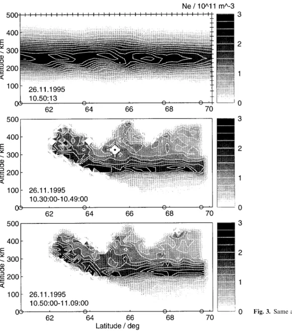
A second example of the ionospheric electron density observed by the two methods is plotted in Fig. 3. In this case the F region contains a series of density enhance-ments which are immediately interpreted as travelling ionospheric disturbances due to gravity waves propagat-ing in the neutral atmosphere. The slanted wave fronts, visible in all three panels between 200- and 300-km alti-tudes, are characteristic of atmospheric gravity waves. Since the wave fronts are tilted southwards from the vertical direction and the source of the gravity waves is most probably at lower heights, we can conclude from the well-known gravity wave theory that the gravity wave propagates in the southward direction. The periods of these waves are typically of the order of 20—60 min, which means that the F region can vary considerably during a single radar scan of 20-min duration. In this case the period is necessarily longer than 20 min, otherwise the
wave fronts would not be so well visible in the radar observation. Based on this consideration, it seems reason-able to assume that the most northern wave front visible in the middle panel lies above Esrange in the bottom panel. This would give a very rough estimate of 30 min for the wave period.
The tomographic observation in the top panel of Fig. 3 starts at the same time as the radar scan in the bottom panel and therefore the reconstruction corresponds to a somewhat later time. The top panel also shows slanted wave fronts south of Esrange and the most northern one must be the same as that in the bottom panel above Esrange. The horizontal wave length determined from this panel is about 250 km.
Similar observations of travelling ionospheric distur-bances by the tomographic method have been previously presented by Markkanen et al. (1995), Pryse et al. (1995) and Cook and Close (1995). Both Markkanen et al. (1995) and Pryse et al. (1995) pointed out that a tomographic analysis is unable to resolve wave fronts lying northwards of the receiver chain or above the most northern site in a situation like that in Fig. 3. This is because the rays passing this region are more or less perpendicular to the wave fronts, so that front-aligned rays are completely missing. Therefore, we cannot conclude that the gravity wave propagates in the present case only within the region south of Esrange. It is likely that there are more wave fronts in the north which are invisible to the tomographic method. As a matter of fact, the bottom panel most probably shows the front end of the next wave front entering the radar field of view from the north.
After having studied this gravity wave case it is useful to go back to Fig. 1 for a closer look. As a matter of fact, even this example represents a southwards-propagating gravity wave. This seems obvious, because three density enhancements are observed in the tomographic recon-struction and the radar measurements show that they propagate southwards. An interesting point is that the southward propagation of the density enhancement would not alone be sufficient for the identification of the wave. Hence we have here an example where the wave would have been unobserved without the tomographic experiment. The horizontal wave length is in this case of the order of 500 km. Figure 2 also shows that the bottom-side gradient is steeper at the profile at the maximum peak value than elsewhere. This is most probably associated with variations in the field-aligned distribution of ioniza-tion at different phases of the gravity wave.
The two examples shown in this paper are from the same day, and the time of Fig. 1 is about 2 h later than Fig. 3. Unfortunately, no satellite flight is available from the interval between these two incidents, and therefore we cannot study whether the two events are separate or whether the gravity wave continues during the gap in the observations.
4 Discussion
The satellite radiotomography is still in a developing state. Various inversion methods are being used and
Fig. 3. Same as Fig. 1
compared to each other. Regardless of the inversion method, the experimental set-up poses a basic difficulty which is associated with the absence of horizontal rays. If the ionosphere is a horizontally stratified layer, this means that the measurements contain hardly any information on the profile height and shape. Then the solution of the tomographic problem greatly depends on additional in-formation, which can be obtained from radar or iono-sonde measurements or model profiles. The situation becomes easier if the ionosphere contains horizontal gradients like those at the edges of the F-region trough or at large plasma enhancements. This can be understood by considering an extreme case of an ionosphere consisting only of a few isolated blobs. If the number of blobs is not too large, their positions could in many cases be solved by a simple triangulation without the help of any inversion algorithm. Hence, roughly speaking, a simple ionosphere is more difficult to measure by satellite tomography than a complicated one.
In practice, the inversion of satellite radiotomography data implies, either consciously or unconsciously, the use of some additional information. In recursive algorithms this is hidden in the start profile and stop criteria in a way which is difficult to quantify. In these methods much effort has been put into finding suitable start profiles. It is also possible to construct the ionosphere from base functions built using model ionospheres. In this case the a priori information is obtained from these models. In the present method the inclusion of the a priori information is made within a well-formulated mathematical framework, which makes it easy to understand its role and to control its effects. One should notice that, although only simple regu-larization profiles are used in the present work, the method and analysis package allow any sophisticated ionospheric model to be applied for this purpose.
The comparisons of incoherent-scatter and satellite tomo-graphy methods given in this paper as well as in some previous works (e.g. Pryse and Kersley, 1992; Markkanen
et al., 1995; Heaton et al., 1995; Mitchell et al., 1995)
convincingly demonstrate the benefit of the satellite tomo-graphy method. Although differences may occur in details, the tomographic method is capable of reconstructing reliably the gross-scale structures of the ionosphere. The mapping takes place quickly within a wide iono-spheric region, which can be extended by adding more receivers to the chain.
Gravity waves are an interesting topic which could be effectively studied using combined tomographic and inco-herent-scatter measurements. The wave period and verti-cal wave length could be reliably measured using the vertical direction of the radar beam and the horizontal wave length, as well as an additional measurement for the vertical wave length, would be obtained from the graphic experiment. Another topic suitable for tomo-graphic studies is the mid-latitude trough. This has been recently shown, e.g., by Mitchell et al. (1995) by comparing tomographic and incoherent-scatter measurements.
Acknowledgements. The authors are grateful to S. M. Chernyakov, J. Pirttila( , E. Saviaro and T. Ulich for assistance in the tomographic measurements, to T. L. Hansen for his great help in arranging the receiver site at Tromsø and to R. Kuula for help in data processing. We are also grateful to L. Kersley and the tomographic group at the University of Wales, Aberystwyth for permission to use their EIS-CAT data. Similarly, the efforts made by the UK and Finnish EISCAT teams, as well as support from the EISCAT staff during the joint EISCAT campaign, are gratefully acknowledged. The EISCAT Scientific association is supported by the Suomen Akatemia of Finland, Centre National de la Recherche Scientifique of France, Max-Planck Gesellchaft of the Federal Republic of Germany, Norges Almenvitenskapelige Forskningsrasd of Norway, Natur-vetenskapliga Forskningsrasdet of Sweden and the Science and En-gineering Research Council of the United Kingdom.
Topical Editor D. Alcayde´ thanks L. Kersley and S. J. Franke for their help in evaluating this paper.
References
Andreeva, E. S., V. E. Kunitsyn, and E. D. Tereshchenko, Phase-difference radiotomography of the ionosphere, Ann. Geophysicae, 10, 849—855, 1992.
Austen, J. R., S. J. Franke, C. H. Liu, and K. C. Yeh, Application of computerized tomography techniques to ionospheric research, in Radio beacon contribution to the study of ionisation and dynamics of the ionosphere and corrections to geodesy, Ed. A. Tauriainen, University of Oulu, Oulu, Finland, Part 1, 25—35, 1986. Austen, J. R., S. J. Franke, and C. H. Liu, Ionospheric imaging using
computerized tomography, Radio Sci., 23, 299—307, 1988. Censor, Y., Finite Series-Expansion Reconstruction methods, Proc.
IEEE, 71, 409—419, 1983.
Cook, J. A., and S. Close, An investigation of TID evolution observed in MACE ’93 data, Ann. Geophysicae, 13, 1320—1324, 1995. Fehmers, G., A new algorithm for ionospheric tomography, in
Proceedings of the International Beacon Satellite Symposium,
ºni-versity of ¼ales, Aberystwyth, ºK, 11—15 July 1994, Ed. L. Kersley, 52—55, 1994.
Fougere, P. F., Ionospheric radio tomography using maximum entropy. 1. Theory and simulation studies, Radio Sci., 30, 429—444, 1995.
Fremouw, E. J., J. A. Secan, and B. M. Howe, Application of stochastic inverse theory to ionospheric tomography, Radio Sci., 27, 721—732, 1992.
Heaton, J. A. T., S. E. Pryse, and L. Kersley, Improved background representation, ionosonde input and independent verification in experimental ionospheric tomography, Ann. Geophysicae, 13, 1297—1302, 1995.
Kunitsyn, V. E., E. S. Andreeva, E. D. Tereshchenko, B. Z. Khudukon, and T. Nygre´n, Investigations of the ionosphere by satellite radiotomography, J. Imag. Syst. ¹echnol., 5, 112—127, 1994. Kunitsyn, V. E., E. D. Tereshchenko, E. S. Andreeva, B. Z. Khudukon,
and Y. A. Melnichenko, Radiotomographic investigations of ionospheric structures at auroral and middle latitudes, Ann. Geophysicae, 13, 1242—1253, 1995.
Lanchester, B. S., T. Nygre´n, A. Huuskonen, T. Turunen, and M. J. Jarvis, Sporadic-E as a tracer for atmospheric waves, Planet. Space Sci., 39, 1421—1434, 1991
Markkanen, M., M. Lehtinen, T. Nygre´n, J. Pirttila~ , P. Henelius, E. Vilenius, E. D. Tereshchenko, and B. Z. Khudukon, Bayesian approach to satellite radiotomography with applications in the Scandinavian sector, Ann. Geophysicae, 13, 1277—1287, 1995. Mitchell, C. N., D. G. Jones, L. Kersley, S. E. Pryse, and I. K.
Walker, Imaging of field-aligned structures in the auroral iono-sphere, Ann. Geophysicae, 13, 1311—1319, 1995.
Pakula, W. A., P. F. Fougere, J. A. Klobuchar, H. J. Kuenzler, M. J. Buonsanto, J. M. Roth, J. C. Foster, and R. E. Sheehan, Tomo-graphic reconstruction of the ionosphere over North America with comparisons to ground-based radar, Radio Sci., 30, 89—103, 1995.
Pryse, S. E., and L. Kersley, A preliminary experimental test of ionospheric tomography, J. Atmos. ¹err. Phys., 54, 1007—1012, 1992.
Pryse, S. E., C. N. Mitchell, J. A. T. Heaton, and L. Kersley, Travelling ionospheric disturbances imaged by tomographic techniques, Ann. Geophysicae, 13, 1325—1330, 1995.
Raymund, T. D., Comparisons of several ionospheric tomography algorithms, Ann. Geophysicae, 13, 1254—1262, 1995.
Raymund, T. D., J. R. Austen, S. J. Franke, C. H. Liu, J. A. Klobuchar, and J. Stalker, Application of computerized tomogra-phy to the investigation of ionospheric structures, Radio Sci., 25, 771—789, 1990.
Raymund, T. D., S. E. Pryse, L. Kersley, and J. A. T. Heaton, Tomographic reconstruction of ionospheric electron density with European incoherent scatter verification, Radio Sci., 28, 811—817, 1993.
Raymund, T. D., S. J. Franke, and K. C. Yeh, Ionospheric tomogra-phy: its limitation and reconstruction methods, J. Atmos. ¹err. Phys., 56, 637—657, 1994.
Vasicek, C. J., and G. R. Kronschnabl, Ionospheric tomography: an algorithm enhancement, J. Atmos. ¹err. Phys., 57, 875—888, 1995.
This article was processed by the author using the LATEX style file
cljour2 from Springer-Verlag.