Development of tropical cyclones from mesoscale convective systems

Development of Tropical Cyclones from Mesoscale

Convective Systems

by

Marja Helena Bister

Filosofian kandidaatti, Meteorology (1991)

University of Helsinki

Submitted to the Department of Earth, Atmospheric and

Planetary Sciences in Partial Fulfillment of the

Require-ments for the Degree of

DOCTOR OF PHILOSOPHY IN METEOROLOGY

at the

MASSACHUSETTS INSTITUTE OF TECHNOLOGY

June 1996

@ 1996 Massachusetts Institute of Technology. All Rights Reserved.

A uthor ...

Department 6f Earth, Atmospheric and Planetary Sciences

March 29, 1996

Certified by ...

Kerry A. Emanuel

Professor of Meteorology

Accepted by ...

Thomas H. Jordan

Department Head

Development of Tropical Cyclones from Mesoscale Convective Systems

by Marja Bister

Submitted to the Department of Earth, Atmospheric and Planetary Sciences on March 29, 1996 in partial fulfillment of the

require-ments for the degree of Doctor of Philosophy in Meteorology

Abstract

Hurricanes do not develop from infinitely small disturbances. It has been suggested that this is because of the effect of downdrafts on boundary layer 8e. The goal of this work is to understand what kind of initial disturbances can induce tropical cyclogenesis. Data from a mesoscale convective system (MCS) that devel-oped into hurricane Guillermo in 1991, were analysed. The MCS was an object of intensive observations during Tropical Experiment in Mexico. Data were collected using two aircraft flying into the MCS every 14 hours. A vortex, strongest in the middle troposphere, with a lower tropospheric humid and cold core, was found in the stratiform precipitation region of the MCS. A negative anomaly of virtual potential temperature and Ee in the boundary layer suggest that the cold anomaly was at least partially owing to evaporation of rain. A hurricane developed from the cold core vortex in about three days.

A nonhydrostatic axisymmetric model by Rotunno and Emanuel was used to study whether evaporation of

precipitation from a prescribed mesoscale showerhead could lead to a vortex with a lower tropospheric humid and cold core. In the model this indeed happens and the cold core vortex develops into a hurricane.

If the showerhead precipitation is weak and stopped too early, the vortex that develops as a result of

evapo-ration barely extends to the boundary layer, and the system barely develops into a hurricane. This suggests that without external forcing, a cold core vortex that does not extend to the boundary layer does not develop into a hurricane. Further experiments were made to test whether the cold core vortex itself or the associated high relative humidity is more important for cyclogenesis. In the model, high relative humidity can make cyclogenesis occur two days earlier, but without the vortex does not lead to cyclogenesis. The cold core favors shallow convection even in the presence of negative anomaly of 8e in the boundary layer, thereby reducing the negative effects of downdrafts when the wind speed is still small.

A simple thought experiment suggests that evaporation lasting for less than the time it takes parcels to

descend through the layer experiencing evaporation leads to a cyclone with an anticyclone below it. This idea is supported by numerical simulations. The thought experiment also suggests that relative flow through the system can prevent downward development of the vortex or even its formation. The prevention of the downward propagation of the vortex could be one reason for the observed negative effect of shear on tropi-cal cyclogenesis. Composite analysis of tropitropi-cal cyclogenesis over western Pacific by Zehr supports the important role of the cold core vortex extending all the way to the boundary layer.

Thesis Supervisor: Kerry A. Emanuel Title: Professor of Meteorology

Acknowledgements

I thank my thesis advisor, Kerry Emanuel, for his guidance, constructive criticism, and going carefully over several drafts of this thesis. I have benefitted greatly from discussions with him on scientific problems within and outside of hurricane research. I would like to thank John Marshall, Dave Raymond from New Mexico Institute of Mining and Technol-ogy, and Earle Williams for serving in my thesis committee, reading the thesis, and sug-gesting many improvements to it. I am also grateful to Jochem Marotzke, Richard Rosen

and Peter Stone for serving in my thesis committee at the early stage of my studies. I am grateful to several people outside of MIT who contributed to this work. Bob Burpee

and Stan Rosenthal gave me the opportunity to work at the Hurricane Research Division of NOAA, where I edited the Doppler wind fields. Frank Marks and John Gamache helped me use the software at the Hurricane Research Division. Richard Rotunno of National Center for Atmospheric Research helped me with my questions about the Rotunno-Eman-uel model.

I benefitted from scientific discussions with many students, particularly Michael Morgan, Nilton Renno, and Lars Schade. I thank Frangoise Robe for discussions related to course-work and our tropical research topics, and especially for her friendship.

Jane McNabb, Joel Sloman, and Tracey Stanelun helped coping with bureaucracy. I thank my father Martti and my sisters Liisa and Anja for their love and support. Martti's encouragement and his example as a scientist have been crucial. I thank my husband Esko Keski-Vakkuri for his love and imagination.

Table of Contents

1 Introduction...13

1.1 Tropical Experiment in Mexico (TEXMEX) and hurricane Guillermo ... 15

1.2 Previous work on tropical cyclogenesis from mesoscale systems...17

1.3 G oals ... 20

2 D ata and analysis m ethods... 23

2.1 D oppler radar data... 26

2.2 In situ data... 32 3 Analysis results ... 35 3.1 Large-scale conditions ... 35 3.2 Flight 2P...41 3.3 Flight 3E ... 44 3.4 Flight 4P... 46 3.5 Flight 5E ... 48 3.6 Flight 6P...51 3.7 Conclusion ... 54 4 N um erical m odel... .57

4.1 Physics of the m odel... 57

4.2 N ew m icrophysics schem e... 60

4.3 N um erics... 63

5 Rainshower sim ulations ... 69

5.1 Control sim ulation ... 72

5.2 Sensitivity studies ... 77

5.3 Comparison of the observations and the control simulation...85

6 The roles of cold core vortices and relative humidity in cyclogenesis ... 87

7 Discussion...-91

7.1 Thought experiment on the downward propagation of vorticity ... 92

7.2 Importance of the outlined process for cyclogenesis in practice ... 97

8 Concluding rem arks ... 105

List of Figures

Figure 2.1: Tracks of aircraft-estimated vortex centers of TEXMEX cases that

developed into hurricanes (D. Raymond, personal communication 1995)...24

Figure 3.1: Infrared images from GOES on 2 August 1991...36

Figure 3.2: Same as in Fig. 3.1, but on 3 August...37

Figure 3.3: ECMWF wind analysis at 00 UTC on 3 August ... 39

Figure 3.4: Radar observations in pre-Guillermo MCS during flight 2P ... 40

Figure 3.5: In situ observations from 3 km altitude in pre-Guillermo MCS during flig h t 2 P ... 4 2 Figure 3.6: In situ observations from 300 m altitude in pre-Guillermo MCS during fligh t 2 P ... 4 3 Figure 3.7: In situ observations from 3 km altitude in pre-Guillermo MCS during fligh t 3E ... 4 4 Figure 3.8: In situ observations from 3 km altitude in pre-Guillermo MCS during fligh t 3E . ... 4 5 Figure 3.9: Radar observations in pre-Guillermo MCS during flight 4P ... 47

Figure 3.10: In situ observations in pre-Guillermo MCS during flight 4P...49

Figure 3.11: In situ observations in tropical storm Guillermo during flight 5E.. ... 50

Figure 3.12: Radar observations in hurricane Guillermo during flight 6P. ... 51

Figure 3.13: In situ observations in hurricane Guillermo during flight 6P...52

Figure 5.1: Maximum of tangential wind as a function of time above the lowest model level and at the lowest model level in the control simulation...72

Figure 5.2: Average of temperature anomaly, relative humidity, and tangential velocity betw een 4 and 8 hours... 74

Figure 5.4: Same as in Fig. 5.2, but average calculated between 20 and 24 hours...76 Figure 5.5: Hurricane in the control simulation... 78 Figure 5.6: Maximum of tangential velocity as a function of time in experiments

DM R, HM R, DA , and H A ... 80 Figure 5.7: Maximum of tangential velocity as a function of time in experiments

HD, HDDMR, and HDDMR with surface fluxes set to 0 outside 340 km...82 Figure 5.8: Maximum of tangential velocity in simulations with the HDDMR-FLUX model with low and high middle tropospheric relative humidity; and with the control simulation model with low and high middle tropospheric relative humidity ... 85 Figure 5.9: Temperature anomaly in the control simulation averaged between 76

and 80 hours...86 Figure 6.1: Schematic illustration of initial conditions in experiments B 1, B2,

an d B 3 ... 8 8 Figure 6.2: Maximum of tangential velocity as a function of time in experiments

B 1, B2, B3, and in experiment with moist column extending to 150 km...89 Figure 7.1: Thought experiment of cooling in a cylinder ... 95 Figure 7.2: Vertical profile of tangential wind in the 1-3 degree band surrounding the center of the cluster (Zehr 1976)... 98 Figure 7.3: Thermal anomalies in the clusters (Zehr 1976)...100 Figure 7.4: Vertical shear in the clusters, and the mean motion of the clusters

(Z ehr 197 6 ). ... 10 1 Figure 7.5: Early convective maximum of Typhoon Abby, 1983 (Zehr 1992)...103

List of Tables

Table 2.1: Summary of flights into (pre-)Guillermo...25 Table 2.2: The characteristics of the NOAA WP-3D aircraft's Doppler radar... 26 Table 2.3: The mean and standard deviations of the differences between in situ and merged D oppler w ind... .... ----..--- .32

Table 3.1: Averages of in situ data in a box around the vortex from the two flight altitudes for flights 2P, 4P, and 6P... ... 53 Table 4.1: Model parameters used in RE and in present simulations...66 Table 5.1: M odel sim ulations... 79

Chapter 1

Introduction

Riehl (1954) noted that tropical cyclones do not form spontaneously, but from distur-bances of independent dynamical origin. Tropical cyclones have often been observed to be triggered by easterly waves (e.g. Shapiro 1977). But only about one out of ten easterly waves develops into a hurricane (Avila 1991). Shapiro (1977) noted that the development of some easterly waves into tropical cyclones may depend on the characteristics of the mean flow. On the other hand, it has been suggested that upper tropospheric potential vor-ticity (PV) anomalies could trigger cyclogenesis. Simpson and Riehl (1981) discuss sev-eral cases of tropical cyclogenesis that are associated with an approaching upper tropospheric trough. However, they also note that in some cases an upper tropospheric trough seems to cause an incipient storm to die. Reilly (1992) studied tropical cyclogene-sis over western North Pacific in summer 1991, and noted that majority of the cases were associated with positive advection of PV in the upper troposphere. Montgomery and Far-rell (1993) have studied the effect of an upper tropospheric PV anomaly on a weak surface cyclone using a balanced model. Their results suggest that an upper tropospheric PV anomaly moving with respect to the lower level winds might result in a spin-up of a weak surface cyclone. Molinari et al. (1995) studied intensification of hurricane Emily associ-ated with an upper tropospheric PV anomaly. Their results suggest that tropical cyclones can intensify as a result of vertical alignment of an upper tropospheric PV anomaly and the cyclone in the lower troposphere. However, they stress that a large-scale upper tropo-spheric PV anomaly would be associated with vertical shear strong enough so that weak-ening of the cyclone would result. They view the upper tropospheric anticyclone associated with the tropical cyclone important in reducing the scale of the approaching

upper tropospheric PV anomaly so that shear associated with the upper tropospheric PV anomaly is small. However, it is still not known how important in practice the upper tropo-spheric PV anomalies are for cyclogenesis, and what the exact mechanism of the possible cyclogenesis associated with these PV anomalies is.

There have been several studies of tropical cyclogenesis using numerical models. However, as noted by Rotunno and Emanuel (1987), in none of the simulations has the model's initial state been neutral to convection. Large available energy for convection has lead to a rapid intensification of very weak perturbations in the wind field (e.g. in the model of Anthes 1972), which is not consistent with the observation that tropical cyclones do not form in the absence of disturbances of independent dynamical origin. Rotunno and Emanuel (1987) studied the nature of tropical cyclogenesis using a model with an initial state that is neutral to model's convection. Their study will be discussed in section 1.1.

In this work I study the problem of tropical cyclogenesis from mesoscale perspective. The results of this work suggest that a long-lasting mesoscale convective system can induce tropical cyclogenesis. More specifically, evaporation of mesoscale precipitation that lasts long enough and is associated with little shear (or more generally, little relative flow through the precipitation region) can lead to a formation of a hurricane. Two impor-tant questions that are not addressed in this study are: 1) What is the mechanism behind the formation and maintenance of long-lived mesoscale convective systems? 2) Is there a relation between upper tropospheric PV anomalies and mesoscale convective systems?

1.1 Tropical Experiment in Mexico (TEXMEX) and hurricane

Guill-ermo

The fact that tropical cyclones develop from disturbances of independent dynamical origin leads to two questions: Why do not tropical cyclones form spontaneously? What kind of initial disturbances can induce tropical cyclogenesis, and how do they form? Rotunno and Emanuel (1987, hereinafter RE) and Emanuel (1989) attempted to answer the first ques-tion. Results from their numerical simulations suggest that convective downdrafts bring air of low equivalent potential temperature (Oe) into the boundary layer, preventing further convection. Therefore, for tropical cyclogenesis to occur, the negative effect of the down-drafts has to be overcome. In principle this might happen owing to an increase of Oe in the middle troposphere, an increase of relative humidity so that evaporation of rain does not occur, or an increase of wind speed so that the sea surface fluxes keep replenishing the boundary layer Oe. Indeed, Emanuel et al. (1994) claim that convection, in quasi-equilib-rium with forcing, can cause positive temperature anomalies only if it is associated with a positive anomaly of sea surface temperature, surface wind speed, or 0e above the subcloud layer, or a negative anomaly in convective downdraft mass flux. The simulations by RE and Emanuel (1989), in which a warm core vortex was used in the initial state, suggested that an increase of 6_{e in the middle troposphere is needed for tropical cyclogenesis to be} possible. The main goal of TEXMEX, a field experiment to study tropical cyclogenesis over eastern North Pacific, was to test a hypothesis stated in the TEXMEX Operations Plan (Emanuel 1991): The elevation of 0e in the middle troposphere just above a near-sur-face vorticity maximum is a necessary and perhaps sufficient condition for tropical cyclo-genesis. It was assumed that the elevation of Oe is accomplished by deep convection bringing high 0e to the middle troposphere, as occurs in the models initialized by warm core vortices. Analysis of one of the TEXMEX cases, a mesoscale convective system that

developed into hurricane Guillermo, showed a moderate increase of Oe at 3 km altitude. The value of Oe remained constant, however, for over a day before rapid strengthening started, suggesting that the observed increase of midtropospheric Oe was not enough to start the intensification. Concerning the TEXMEX hypothesis, the role of downdrafts had certainly been diminished owing to the positive anomaly of Oe and relative humidity in the initial vortex. But since the increase of midtropospheric Oe was not enough to start the intensification it is clear that in this case the increase of Oe is not a sufficient condition for tropical cyclogenesis.

The goal of this work is to answer the second question posed on tropical cyclogenesis. What kind of initial disturbances can induce tropical cyclogenesis, and how do they form? The basis for this study are the observations made in the disturbance that developed into tropical cyclone Guillermo. The initial perturbation was found in a mesoscale convective system (MCS). Houze (1993, p. 334) defines an MCS as a cloud system that occurs in connection with an ensemble of thunderstorms and produces a contiguous precipitation area of 100 km or more in horizontal scale in at least one direction. MCSs typically last from hours to days, and consist of deep convective clouds, and a stratiform precipitation region. The stratiform precipitation falls from an anvil cloud. The anvil cloud consists in part of debris from deep convective clouds. There is also condensation in the anvil cloud that increases the stratiform precipitation. The depth of the anvil cloud varies, but the base is often close to the isotherm of 0 C, that resides near 5 km altitude.

The disturbance that developed into hurricane Guillermo was very different from the warm core disturbance used in the initial state in the simulations on which the TEXMEX hypothesis was based. A vortex, with cyclonic wind increasing with height in the lower troposphere, was found in the stratiform precipitation region of the MCS. The vortex had a cold core in the lower troposphere. At 3 km altitude relative humidity was anomalously

high. The data from the pre-Guillermo mesoscale system were collected over a period of 3 days. The humid cold core vortex existed already at the time of the first flight. A warm core system developed within the cold core and intensified into a hurricane during the period of intensive observations. To our knowledge, this is the best data set documenting the development of a weak lower tropospheric cold core vortex into a hurricane.

1.2 Previous work on tropical cyclogenesis from mesoscale systems

The understanding of tropical cyclogenesis has traditionally meant the understanding of the increase of vorticity. A positive anomaly in vorticity is associated with increased sea surface fluxes owing to higher wind speed, and a decreased Rossby radius of deformation (e.g. Chen and Frank 1993). The former enhances convection, and the latter increases the local increase of temperature associated with convection. The role of relative humidity has been less studied, perhaps due to the observation that midtropospheric relative humid-ities do not differ in large-scale environments of convective systems which intensify into hurricanes and those which do not (McBride and Zehr 1981). Tropical disturbances that develop into named storms have been observed to exist in an environment of very weak vertical wind shear (Gray 1968). The negative effect of vertical wind shear has often been explained by "ventilation". Heating associated with deep convection is said to be advected away from the disturbance if vertical shear is large (with vertical shear the whole storm cannot move with the mean wind). Another effect of vertical wind shear could be the tilting of the potential vorticity anomaly associated with the storm (Jones 1995).

Based on these climatological aspects of cyclogenesis, it has been natural that studies aiming at understanding tropical cyclogenesis have concentrated in the formation of vor-ticity. It has been argued that vorticity associated with easterly waves might be conducive to cyclogenesis. Indeed, tropical cyclogenesis over the eastern Pacific is often associated

with easterly waves (Miller, 1991). As discussed before, the second possible source for vorticity is upper tropospheric potential vorticity anomalies. However, there was no evi-dence in the ECMWF data of independent upper tropospheric positive potential vorticity anomalies in the region where hurricane Guillermo formed (Molinari, personal communi-cation 1996). The MCS from which hurricane Guillermo developed formed while an east-erly wave was propagating into the eastern Pacific from the Caribbean Sea (Farfan and Zehnder, 1996, hereinafter FZ). The easterly wave and its interaction with topography may have been important factors in increasing vorticity initially, as suggested by FZ.

Early research into tropical cyclogenesis (see Handel 1990 for an extensive review) assumed that the increase of vorticity occurs owing to convergence into deep convection, and is associated with heating. Lately it has been recognized that vorticity production associated with convection usually takes place in the stratiform precipitation region of MCSs. Midtropospheric vortices have been observed in circular MCSs (e.g. Bartels and Maddox, 1991), and also in squall lines (e.g. Gamache and Houze, 1985). It has been sug-gested that these vortices may be due to vertical heating gradients in the stratiform precip-itation region. On the other hand, results of numerical simulations of a squall line by Davis and Weisman (1994) suggest that line end vortices can form owing to horizontal heating gradients acting on initially horizontal vorticity. Chen and Frank (1993) simulated the for-mation of a midlevel vortex in a midlatitude MCS. In their model the development of a vortex occurs as a response to a vertical heating gradient in the presence of anomalously small local Rossby deformation radius. The small Rossby deformation radius is owing to decreased vertical stability in the anvil cloud. The decreased stability decreases the group speed of gravity waves, thereby preventing spatial dispersion of energy. Therefore, heat-ing in the anvil could lead to a balanced vortex.

There is a relation between MCSs and tropical cyclogenesis. Both mesoscale convec-tive complexes (Velasco and Fritsch, 1987) and tropical cyclones (Zehnder and Gall, 1991) are more frequent over the eastern North Pacific than in the Caribbean. There is also ample evidence in satellite imagery of mesoscale convective complexes leading to tropical cyclogenesis (e.g. Velasco and Fritsch, 1987 and Laing and Fritsch, 1993). In addition, there is in situ data of tropical cyclogenesis from mesoscale convective systems with a midlevel vortex. Bosart and Sanders (1981) studied a midlatitude MCS in which a midlevel vortex had developed. The vorticity extended to quite low altitudes but there was no evidence of surface circulation before the system was over the ocean. Later, over the ocean, the system developed into a storm resembling a tropical cyclone. Moreover, obser-vations by Davidson et al. (1990) show that the AMEX tropical cyclones Irma and Jason initially had maximum intensity in the middle troposphere.

Since tropical cyclones have been observed to develop from MCSs with a midtropo-spheric vortex, the important question becomes how the midlevel vortex leads to a forma-tion of low level vorticity. In Chen and Frank's study of the formaforma-tion of a vortex in a midlatitude MCS, the midlevel vortex descends downward. They associate the downward movement of the midlevel vortex with the downward development of updraft and warm core in the stratiform rain region. By as early as 8 h of simulated time the warm core struc-ture extends down to 850 hPa. This rapid downward extension of the warm core is unlike what was observed in the pre-Guillermo MCS, where it takes about two days for the warm core to develop in the lower troposphere. It must be noted that Chen and Frank's initial condition was characterized by a large value of CAPE and a very moist lower troposphere. It is unlikely that this kind of downward development could occur in an environment with a dry middle troposphere.

Mapes and Houze (1995) have noted that the downward development of the midlevel vortex could be a natural consequence of convection occurring in the region of the midlevel vortex. This idea is based on observations of divergence in a rainband of cyclone Oliver, 1993. Convection in the rainband adjusts itself to oppose temperature perturba-tions in the rainband, implying large convective heating in the cold region, and less heat-ing above the cold region. The associated divergence would tend to increase vorticity close to the surface and decrease it above the cold core. However, they do not explain how convection would form in the region of the midlevel vortex. The downdraft, in the strati-form precipitation region, brings low 8e air to the boundary layer, which tends to prevent convection. It is important to explain how convection can ensue when Oe has a negative anomaly in the boundary layer.

1.3 Goals

The basis of TEXMEX was the prediction of numerical models that the downdrafts owing to evaporation of precipitation and detrainment of cloud are a key factor in preventing tropical cyclogenesis. Since the relative humidity of the initial system, as well as Oe, was elevated, it was natural to assume that the effect of downdrafts on the boundary layer 8e would be minor, and that tropical cyclogenesis would be favored by these thermodynamic factors. Indeed, Emanuel (1995) has found that if a whole atmospheric column of 150 km in radius is saturated, a hurricane forms in a couple of days from an initial vortex with 3 ms-1 maximum wind. On the other hand, earlier research has concentrated on the forma-tion of the midlevel vortex and its downward development. And, as we have seen, there is plenty of evidence of tropical cyclones developing from MCSs with midlevel vortices.

The perturbation from which hurricane Guillermo developed was associated with both a cold core vortex and high relative humidity. The goal of this work is to shed light on the

following questions: How did the initial disturbance with a humid cold core vortex develop? How did the midlevel vortex descend downward? Is the existence of a humid cold core vortex, as observed in pre-Guillermo, a suitable initial disturbance for cyclogen-esis? And if it turns out it is, is the high humidity or the vortex itself more important for cyclogenesis?

An overview of TEXMEX is given in Chapter 2. Also the sources of data, and analysis methods are discussed in Chapter 2. Results from the data analysis are presented in Chap-ter 3, in which the development of the pre-Guillermo disturbance into a hurricane is docu-mented. The numerical model that I use to study the formation of the initial humid cold core vortex, and the relative importance of humidity and a cold core vortex, is described in Chapter 4. Chapters 5 and 6 contain results from the numerical simulations. In Chapter 5, results from simulations designed to improve our understanding of the formation of the initial humid cold core vortex, and its possible development into a hurricane are discussed. The relative importance of the humidity and the cold core vortex is addressed in Chapter 6.

The numerical simulations, presented in Chapter 5, suggest that a humid cold core vor-tex can be a result of evaporation of mesoscale precipitation, and that the vorvor-tex, formed in this way, is a suitable initial disturbance for tropical cyclogenesis. Results from Chapter 6 suggest that the vortex is more important for cyclogenesis than increased relative humid-ity. Sensitivity simulations suggest that if the vortex does not extend to the surface when the mesoscale precipitation ends, a hurricane will not form. In Chapter 7, a thought exper-iment that captures the crudest aspects of the downward propagation of a cold core cyclone is discussed. The thought experiment reveals some factors that affect the down-ward development, and gives a possible reason why vertical shear is unfavorable for trop-ical cyclogenesis. The likelihood that the mechanism for troptrop-ical cyclogenesis outlined in

this work would frequently be accountable for tropical cyclogenesis is discussed in light of observational work by Zehr (1976 and 1992) in Chapter 7. Chapter 8 contains conclud-ing remarks.

Chapter 2

Data and analysis methods

In TEXMEX measurements were made inside developing and nondeveloping cloud clus-ters, using the WP-3D aircraft operated by the NOAA Office of Aircraft Operations (OAO) and the National Center for Atmospheric Research (NCAR) Lockheed Electra. Both aircraft were equipped to make in situ measurements of standard meteorological variables, and the WP-3D had the additional capability of deploying omega dropwin-sondes and making detailed Doppler radar measurements. The aircraft measurement sys-tems are described in detail in the TEXMEX Operations Plan (Emanuel 1991).

The eastern tropical North Pacific region was selected for the field program. This region has the highest frequency of genesis per unit area of any region worldwide (Els-berry et al., 1987). The field phase of the experiment began on 1 July and ended on 10 August 1991. During the project there were 6 Intensive Operation Periods (IOP's) that surveyed 1 short-lived convective system, 1 nondeveloping mesoscale cloud cluster, and 4 clusters that ultimately developed into hurricanes. The tracks of those systems that devel-oped into hurricanes are shown in Fig. 2.1. Description of the aircraft flight operations are provided in the TEXMEX Data Summary (Renn6 et al. 1992).

As the TEXMEX hypothesis concerned thermodynamic transformations of the lower and middle troposphere, most flight operations were conducted near the 700-hPa level and in the subcloud layer. Most of the NOAA WP-3D flights at 700 hPa deployed omega drop-winsondes, and the tail Doppler radar on the WP-3D operated almost uninterrupted through all of the flight operations. The aircraft flew alternating missions at approximately

14-hour intervals. Most flight missions lasted 7-9 hours, of which 1-3 hours were used in transit to the target area.

5 U J I I .

-110 -105 -100 -95 -90

Figure 2.1: Tracks of aircraft-estimated vortex centers of TEXMEX cases that developed into hurricanes (D. Raymond, personal communication 1995). Circle shows where each disturbance was declared a tropical storm by National Hurricane Center. E is for Enrique,

F for Fefa, G for Guillermo and H for Hilda.

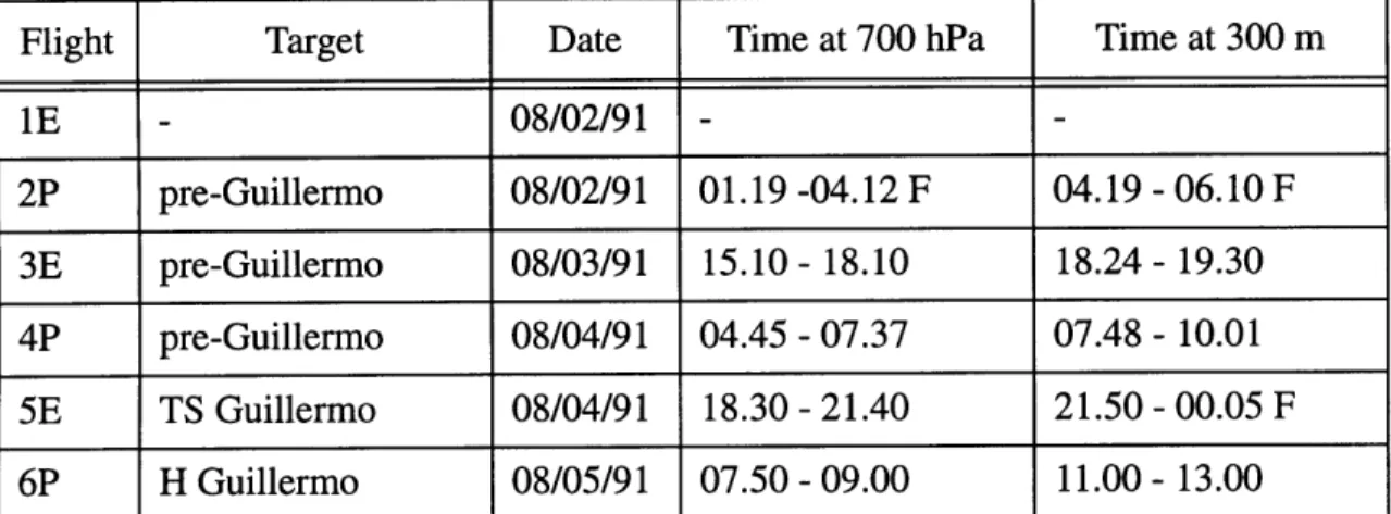
The MCS that developed into hurricane Guillermo was chosen as the case study of this work because of the very good data coverage, and the very early state of the system during the first flight, as well as the interesting cold core structure of the storm. The MCS that developed into hurricane Guillermo on 5 August 1991 was the target object of IOP 5 from 2 August 1991 to 5 August 1991. Six flights were flown during IOP 5. The first, third, and fifth flights were flown with the Electra. These flights are labeled lE, 3E, and 5E, respec-tively. The second, fourth, and sixth flights were flown with the WP-3D. These flights are

labeled 2P, 4P, and 6P, respectively. The flights are summarized in Table 2.1. Each flight consisted of several flight legs at 3 km altitude (700 hPa), and several more at 300 m. The

first flight, 1E, was conducted well to the west of the developing system.

Flight Target Date Time at 700 hPa Time at 300 m

1E - 08/02/91 - -2P pre-Guillermo 08/02/91 01.19 -04.12 F 04.19 -06.10 F 3E pre-Guillermo 08/03/91 15.10 - 18.10 18.24 - 19.30 4P pre-Guillermo 08/04/91 04.45 - 07.37 07.48 - 10.01 5E TS Guillermo 08/04/91 18.30 - 21.40 21.50 -00.05 F 6P H Guillermo 08/05/91 07.50 - 09.00 11.00 - 13.00

Table 2.1: Summary of flights into (pre-)Guillermo. F is for following day, TS is for tropical storm, and H is for hurricane

In the anvil precipitation the relative humidity measurements of the ODWs often showed 100% relative humidity, indicating wetting of instruments. Owing to the wetting, ODW data is not used in the data analysis. Radar composites from the WP-3D C-band radar, with antenna scanning in the horizontal plane, are used to get an overview of con-vection during the flights. Geostationary Operational Environmental Satellite (GOES) imagery and analysis of wind from the European Centre for Medium-Range Weather Forecasts (ECMWF) were obtained from Farfan and Zehnder of the University of

2.1 Doppler radar data

2.1.1 Doppler radar and its operation

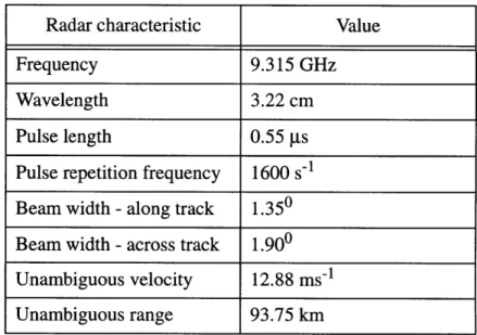
The characteristics of the WP-3D Doppler radar are given in Table 2.2. The unambiguous range and velocity are dictated by the pulse repetition frequency and the wavelength. The number of samples per each radar grid volume depends on the distance of the grid volume from the aircraft. There are at least 32 samples per each radar grid volume. The number of samples per grid volume increases with distance from the aircraft, being 128 for distances larger than 38.4 km.

Table 2.2: The characteristics of the NOAA WP-3D aircraft's Doppler radar.

At least two beams from different angles are needed for the determination of the three dimensional wind. The usual method is to fly an L-pattern around the target object, keep-ing the antenna pointkeep-ing angle perpendicular to the aircraft's ground track. This method has been used widely (e.g. Jorgensen et al. 1983, Marks and Houze 1984 and 1987). Another option is to use a Fore/Aft Scanning Technique (FAST). In FAST, the antenna tilt

Radar characteristic Value

Frequency 9.315 GHz

Wavelength 3.22 cm

Pulse length 0.55 gs

Pulse repetition frequency 1600 s-1

Beam width - along track 1.350

Beam width - across track 1.900

Unambiguous velocity 12.88 ms-1 Unambiguous range 93.75 km

angle, defined forward or aft from the perpendicular to the ground track, is changed between each rotation of the antenna about the aircraft's longitudinal axis. The WP-3D Doppler radar was operated using FAST in TEXMEX.

Since the antenna rotates at 10 RPM and the aircraft flies at a speed of 130 ms-1, each revolution of the antenna in the same direction is separated by 1.6 km. The difference in time of two radials pointing to the same point at 80 km from the track is about 7 minutes. The difference is naturally much smaller than the one achieved by using the method of fly-ing the L-pattern.

When FAST is used Doppler velocities are contaminated by the component of the velocity of the aircraft in the direction of the antenna. Thus, wind measurement is prone to errors in the aircraft's ground velocity. On the other hand, the FAST mode is practical when it is not possible to plan the flight pattern in advance. This is because the two com-ponents of the wind can be retrieved from one flight leg.

2.1.2 Editing

The Doppler data were mapped to a 3 x 3 x 0.5 km grid (0.5 km in the vertical direction) by averaging the data in the horizontal direction and interpolating in the vertical direction. The components of the aircraft's ground velocity and precipitation particle fallspeed in the direction of the antenna were subtracted from the radial velocities. Terminal fallspeed was estimated using empirical fallspeed -radar reflectivity relations for ice particles (Atlas et al. 1973) and for liquid water (Joss and Waldvogel 1970). These relations were also used by Marks and Houze (1987). The location of the radar bright band was used to determine where the precipitation was in the form of ice and where it was in the form of liquid. The depth of the bright band was estimated to be about 1.5 km. It was assumed that all precip-itation was in the form of liquid below the bright band, and in the form of ice above it. In

the bright band region the two estimates were combined linearly.

The velocities were then unfolded automatically using Bargen and Brown's method (1980). An independent measure of the wind speed is needed to unfold the velocities. The in situ measurement of wind was used for this purpose. Manual editing of the data fol-lowed the automatic unfolding. Possible wrong unfolding was corrected for by adding a suitable number of unambiguous velocities (see Table 2.2) to any suspicious values. If the velocity still seemed unrealistic, the observation was deleted. Most of the deleting was done at 0.5, 1, and 1.5 km altitudes. Suspicious looking winds at higher altitudes were rel-atively rare, and probably owing to second or multiple trippers, or sidelobes. These errors will be discussed in section 2.1.3. Turning the aircraft in the middle of the flight leg also caused portions of the Doppler winds to be of poor quality, since the angle separation of the two radials was small. Fortunately, this problem occurred only once. The three-dimen-sional wind was calculated from the two radial components in the following way (the computer program was written by John Gamache of Hurricane Research Division/ NOAA): First, the horizontal wind components were calculated assuming that the vertical component is zero. Then, the horizontal components were used to calculate the first guess of the divergence field. Starting from the lowest level, the following procedure was repeated for each level until a prescribed accuracy was attained or until 50 iterations had been done. The vertical wind component for the first iteration was calculated from the anelastic continuity equation using vertical wind velocities from the level below, and the first guess estimate of divergence at the current level. Then, the three wind components were adjusted using the Least Squares method. The solution using this method usually converged to the desired accuracy in less than 50 iterations.

The data from separate flight legs had to be merged in a suitable way for the analysis of the whole MCS. To get a translation velocity of the system, the vortex center was

tracked from one flight to the next. This translation velocity was then used to move the data to appropriate locations at some reference time. If more than one datapoint was moved to the same gridvolume, an average was calculated. The data were mapped to a 5 x 5 x 0.5 km grid, 0.5 km being the vertical resolution. The possible evolution of the MCS while data were being collected was not accounted for. The MCS was long-lived, and the observed vortex within the MCS was at least qualitatively in balance with the mass field (see Chapter 3). Therefore, it is unlikely that there had been large changes in the mesos-cale structure during the couple of hours that the aircraft flew in the MCS during each flight.

2.1.3 Error analysis

The across-track beamwidth (see Table 2.2) corresponds to 0.5, 1, and 2 km at ranges 15, 30, and 60 km, respectively. Thus, smearing of features is expected at large ranges. Note that the flight legs were typically about 60 km apart, and they were always parallel. Radar return from the sidelobes, 15' from the center of the main lobe, can introduce errors to the data, especially in the region of sparse data and sea clutter. Sea clutter can affect the data far from the aircraft, and when the antenna is pointed downward. When the aircraft flies at 3 km altitude and the antenna is pointed horizontally the mainlobe of the beam will touch the sea surface at 90 km range. (The energy in the sidelobe can return from the sea surface from even smaller ranges, though.) The sea clutter contamination becomes a worse prob-lem when the antenna is pointed downward. For example, when data are collected from an altitude of 1.5 km above the sea surface and the flight altitude is still 3 km the mainlobe touches the sea surface as close as 45 km from the aircraft. The Doppler velocities in the case studied were noisy below 2 km altitude. Where data from below 2 km was used in the analysis, care was taken that any suspicious-looking wind was deleted. In addition to sea

clutter and sidelobe problems, second and multitrippers, i.e. return coming form farther than the unambiguous range, can affect the data. Also, errors in terminal fallspeed esti-mates can affect the wind data.

Airborne radars have additional error sources compared to ground based radars. The error in the antenna pointing angles relative to the aircraft are smaller than 0.5' (Marks, 1991 personal communication), and can be accounted for. The antenna position with respect to the ground is calculated using information of the aircraft attitude, given by the Inertial Navigation System. The aircraft attitude angles have errors less than 0.5'. The location and velocity of the aircraft are retrieved by integrating the accelerations given by the Inertial Navigation System. The ground velocity of the aircraft is subtracted from the Doppler velocities to eliminate the velocity component that is owing to the movement of the Doppler radar itself. Therefore, errors in the ground velocity will introduce errors in Doppler winds.

There is an independent source of wind data, which is the aircraft in situ measurement. The accuracy of the Doppler data is assessed by comparing the Doppler velocities to the in situ wind measurements. However, there are two types of errors that cannot be assessed by this comparison: those owing to errors in the ground speed of the aircraft and those owing to errors in terminal fallspeed estimates. First, when there is an error in the ground veloc-ity of the aircraft, the associated error in the in situ wind is as large as in the Doppler wind since the in situ wind is calculated as a difference between true air speed and aircraft ground speed. Second, the error in the Doppler velocities due to errors in the estimated ter-minal fall speed of precipitation particles does not show up in the comparison, because when the antenna points horizontally, as it does when data is collected from the flight alti-tude, the component in the radial velocity due to terminal fallspeed is zero.

Merceret and Davis (1981) estimated the error in the ground speed to be at maximum 4 ms-1. The error is now estimated to 2-3 ms-1 (B. Damiano 1992, personal communica-tion). The error introduced to Doppler velocities owing to an error in the ground speed is constant with height. Therefore, vertical differences of wind are not affected. Assuming an error of 1 ms-1 in the terminal fallspeed (see Atlas et al. 1973), the associated error in the horizontal wind speed for different ranges and elevation angles can be estimated. The errors are less than 1 ms-1 for horizontal distances of more than 4 km from the flight track, assuming that no data farther than 4 km above or below the aircraft is used in the analysis. Moreover, for straight flight tracks this error is perpendicular to the flight track and shows up as spurious divergence or convergence.

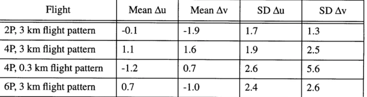
The net effect of other errors than those associated with uncertainties in the ground speed and terminal fallspeed estimates is obtained in the following way: First a 3 km run-ning mean of the in situ wind components was calculated. Then the values were linearly interpolated to those longitudes (latitudes, if leg happened to be oriented more in N-S direction) with gridded Doppler winds. The Doppler winds were then linearly interpolated to the latitudinal positions of the in situ winds. The mean differences and standard devia-tions were calculated for each flight separately. The results for the comparison of the in situ winds and Doppler winds merged from different flight legs are shown in Table 2.3. Note that some errors associated with the Doppler winds are expected to increase with dis-tance from the aircraft. Therefore, a comparison of in situ wind and Doppler wind using only data from the particular flight track would not reveal these errors. However, when merged Doppler winds are used, Doppler data are usually a combination of data from dif-ferent flight legs, even at the location of the flight track

The mean difference between in situ and merged Doppler wind components is always less than 2 ms-1. However, the more interesting quantity is the standard deviation since it

is better related to the errors in the vorticity and divergence. The standard deviations are typically less than 2.5 ms-1. However, for the boundary layer pattern of flight 4P the dif-ference in the meridional component is 5.6 ms-1_{. This most likely reflects a large error in}

the Doppler winds, as will be discussed in Chapter 3.

Flight Mean Au Mean Av SD Au SD Av

2P, 3 km flight pattern -0.1 -1.9 1.7 1.3

4P, 3 km flight pattern 1.1 1.6 1.9 2.5

4P, 0.3 km flight pattern -1.2 0.7 2.6 5.6

6P, 3 km flight pattern 0.7 -1.0 2.4 2.6

Table 2.3: The mean and standard deviations of the differences between in situ and merged Doppler wind components

In summary, the error in Doppler winds associated with the ground speed is at maxi-mum 2-3 ms-1_{. This error is constant with height, and does not affect vertical differences}

of wind. The errors associated with wrong estimates of terminal fallspeeds are less than 1 ms-1 _{farther than 4 km from the flight track, and would mostly show up as spurious}

con-vergence of dicon-vergence. The other errors and their standard deviations are less than 2.5 ms-1, except for the boundary layer pattern of flight 4P.

2.2

In situ data

Intercomparison of instruments onboard the NOAA WP-3D and the NCAR Electra was made using data from two sets of intercomparison flights in the beginning and at the end of the field experiment. The differences between the temperatures and the dew point tem-peratures measured by the two aircraft were less than 0.3 K both in the beginning and at

the end of the field experiment. These differences were accounted for, in the data analysis, by interpolating the differences in time and subtracting them from the data of the other air-craft.

Air that is part of an active convective updraft or downdraft should not be included in the thermodynamic analysis since air in updrafts and downdrafts is just passing through the altitude from which data were collected. Therefore, data were excluded if the magni-tude of vertical velocity exceeded 1 ms-1. Data were also excluded if the measured dew point temperature exceeded the measured temperature. However, no data were excluded from the 300 m analyses, nor were any data excluded from the analysis of thermodynamic fields from flight 6P, since the vertical velocity so often exceeded 1 ms-1 during this flight. Using the same method as with the Doppler data, the data were renavigated to the appro-priate locations at a given time, and 80-second (10 km) averages were calculated. These averages were then analyzed by hand.

Chapter 3

Analysis Results

The study by Farfan and Zehnder (1996) suggests that the easterly wave that was approaching the Eastern Pacific and its interaction with the Sierra Madre mountains increased vorticity in the vicinity of the MCS from which hurricane Guillermo formed. However, not all easterly waves lead to cyclogenesis. On the other hand, MCSs with midlevel vortices have been observed to lead to tropical cyclogenesis. The formation of a large and persistent MCS, even though possibly dependent on large-scale flow, might be enough to lead to tropical cyclogenesis. The analysis of data to be presented in this chapter will indeed justify pursuing the hypothesis that phase changes in the MCS may have been crucial for the formation of hurricane Guillermo. However, it is important to note the fac-tors that contributed to the formation of the MCS are beyond the scope of this work and are left for future work.

3.1 Large-Scale Conditions

3.1.1 Satellite imagery

The mesoscale system developed over the Honduras-El Salvador border during the night of 1-2 August 1991. At 04 UTC on 2 August there is still practically no convection associ-ated with it over the ocean. In Fig. 3. la the infrared image from GOES is shown at 08 UTC on 2 August, 1991. At this time convection is spreading over the ocean and develop-ing into a NNE-SSW oriented line extenddevelop-ing southward from the coast. However, after a few hours the mesoscale system lost its line-like appearance (see Fig. 3.1 b and c). There is some suggestion in the satellite imagery of a convective line separating from the rest of

c) d)

DW CW

Figure 3.1: Infrared images from GOES at (a) 08 (b) 12 (c) 16 (d) and 20 UTC on 2 August 1991. In (c) the estimate of the location of the vortex center based on Doppler wind field is shown with letters DW, and the estimate based on cloud track wind field is

shown with letters CW. The latter estimate is from FZ.

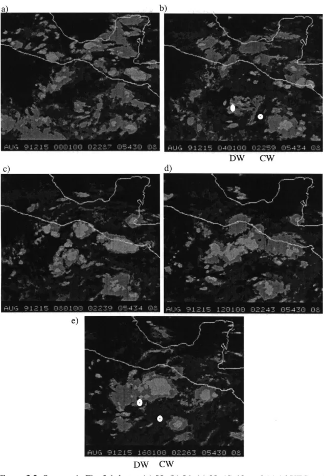
the MCS and propagating rapidly westward leaving the rest of the MCS behind (Figs. 3.1 c and d, and Fig. 3.2a). The convective line seems to weaken while the rest of the MCS

DW CW

c) d)

e)

DW CW

Figure 3.2: Same as in Fig. 3.1, but at (a) 00, (b) 04, (c) 08, (d) 12, and (e) 16 UTC on 3 August. The estimated locations of the vortex are shown in similar fashion as in Fig. 3.1

reintensifies (Figs. 3.2 b, c, and d). The few hours after the formation of the MCS is the only time when satellite imagery suggests a linear organization of the system.

In Figures 3. 1c, 3.2b, and 3.2e estimates of the location of the vortex are shown. Esti-mates are obtained from two sources. FZ estimated the location of the vortex from the cloud track wind field at 14 UTC on 2 August and 14 UTC on 3 August, using visible sat-ellite images. I obtained the locations of the center at 04 UTC on 3 August and 07 UTC on 4 August, using an objective analysis of vorticity of the Doppler wind field. In Figures 3. 1c and 3.2e the location of the vortex using Doppler wind field has been obtained by extrapolation and interpolation of the data, respectively. In Fig. 3.2b the estimate of the location of the vortex using the cloud track wind field has been obtained by interpolation. It would seem that there are two centers about 200 km apart from each other. However, the estimate of the center using cloud track wind field is more uncertain than the estimate using Doppler wind field. For example, at 14 UTC on August 2 the center using the cloud track wind field should be within 90.0 W and 92 W, and 91.0 W was chosen as the most likely location (L. Farfan, personal communication, 1996).

Note that the vortex center estimated using the Doppler wind field is always in the region of the convection associated with the MCS. However, convection is typically stron-ger to the north of the vortex than to the south.

3.1.2. Vertical shear and midtropospheric humidity

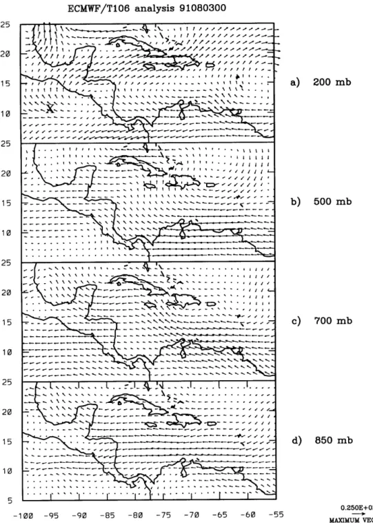
The ECMWF wind analysis at 00 UTC on 3 August 1991 is shown in Figure 3.3. An east-erly wave can be seen near Cuba. The region where the vortex was observed during flight 2P at 04 UTC on 3 August is characterized by small vertical wind shear below 500 hPa. There may have been shear associated with the line of convection that is the first

ECMWF/T106 analysis 91080300 \ \ tt ~ /- - - - -- -- ---- I I---- - -- --- - s - -- -- -. . . .J ,,, -. . . N . . r - - T -100 -95 -90 -85 -80 -75 -70 -65 -60 -55 a) 200 mb b) 500 mb c) 700 mb d) 850 mb 0.250E+02 MAXIMUM VECTOR

Figure 3.3: ECMWF wind analysis at 00 UTC on 3 August, 1991. Location of the vortex is shown in the 200 hPa analysis at 04 UTC on 3 August (cross).

stage of the mesoscale system. However, the rapid disintegration of this line suggests that any shear associated with it has been short-lived. Therefore, we have little reason to believe that horizontal vorticity played a dominant role in the intensification of the vortex.

91Q2 txmec 0334 -G415 GMT 42-4* -96 'K '\\~ ~ 'K f ___ ft _ -95 -94

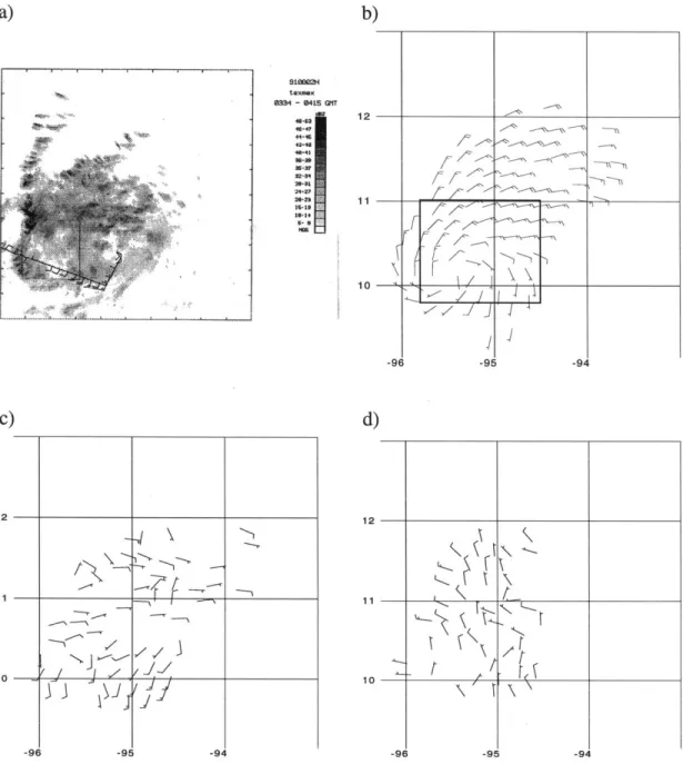
Figure 3.4: Radar observations in pre-Guillermo MCS during flight 2P. (a) Radar reflec-tivity composite from C-band radar, tick marks: 48 km (b) Doppler wind field at 2 km, (c) change of wind from 1 to 3 km, (d) change of wind from 5 to 7 km. Only values larger than 3 ms-I plotted in (c) and (d). Radar data were collected while the aircraft was flying at

Both flights 1E and 2P found regions around the mesoscale system where e was about 330 K and the relative humidity was about 50% at 700 hPa, showing that the middle troposphere in the environment of the MCS was rather dry.

3.2 Flight 2P

The first flight, 1E, was conducted well to the west of the vortex, and on the westernmost part of the MCS. Flight 2P was the first flight into the MCS. In Fig. 3.4, reflectivity mea-sured with the C-band radar and wind meamea-sured with the Doppler radar are shown. Fig-ures 3.4a and b show that the mesoscale vortex is in the stratiform region of the precipitation. There is a bright band in the radar reflectivity (not shown) except to the west and north of the vortex, where the values of radar reflectivity are large. Assuming that the vortex is in balance with the thermal field, the change of wind in vertical direction can be used as a proxy for the thermal anomalies in the corresponding layer. The thermal wind relation for flow in hydrostatic and gradient wind balance (e.g. Emanuel 1989) is

1 (m2 -R

(T,

1 _(3.1)

r3 F r V (JJ } P

where M = (0.5

f

radius, p is pressure, Tv is virtual temperature, v is tangential velocity, and R is the gas constant for air. If the vertical wind shear is anticyclonic (cyclonic), the vortex has a warm (cold) core. The vertical difference between the wind at 3 km and 1 km (Fig. 3.4c), with southwesterly wind difference on the southern side of the vortex and easterly wind differ-ence on the northern side of the vortex, suggests that the vortex is associated with a cold

core in the lower troposphere. The vertical difference between the wind at 7 and 5 km (Fig. 3.4d) suggests a warm core in the upper troposphere, associated with the vortex.

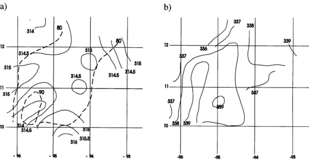
In situ observations from 3 km altitude are shown in Figure 3.5. Relative humidity is about 90% in the region of the vortex. The analysis of virtual potential temperature con-firms the existence of a cold core associated with the vortex in the lower troposphere. Oe is relatively uniform with a maximum value of 339 K collocated with the cold and humid core in the center of the vortex. Note that the values of Oe are about 8 K higher than the values found in the environment of the MCS during flights 1E and 2P, and the values of relative humidity are remarkably higher than the value of 50% found in the environment during same flights.

Figure 3.5: In situ observations from 3 km altitude in pre-Guillermo MCS during flight 2P. (a) Virtual potential temperature, solid, and relative humidity in percents, dashed; (b)

The analyses of ee and virtual potential temperature in the boundary layer are shown in Fig. 3.6. In the region of the vortex, both variables have negative anomalies. The nega-tive anomaly of virtual potential temperature in the region of the vortex (see also Fig. 3.4c which implies a negative anomaly in the layer from 1 to 3 km), and the fact that the cold core vortex is found in the stratiform precipitation region suggest that phase changes, especially evaporation and melting of precipitation, could be responsible for the cold core vortex. In principle, adiabatic ascent could also result in a lower tropospheric cold core, with a positive anomaly in relative humidity. However, the fact that the cold anomaly extends to 300 m and is associated with a negative anomaly of 8e at the same altitude is more consistent with a downdraft owing to evaporation of rain and perhaps melting of ice.

a) b) 12- 12 304 342 k6- 303 10 N344 46-5-4-96 -96 -4

Figure 3.6: In situ observations from 300 m altitude in pre-Guillermo MCS during flight 2P. (a)

Oe,(b)

3.3 Flight 3E

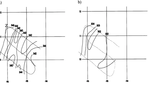
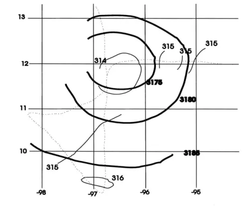
Owing to the less than optimal flight pattern at 3 km altitude, it is difficult to locate the center of the vortex by looking at the wind field (not shown). However, analysis of the height field of the 700 hPa surface seems to crudely resolve the low pressure center of the vortex. The aircraft flew within a few hectopascals of the 700 hPa level. A correction to 700 hPa was made using the hydrostatic equation and the measured pressure and tempera-ture. The variation of the values of height in Fig. 3.7 corresponds to 2 hPa. The field of vir-tual potential temperature shows that the low pressure center is associated with a cold core. Values of virtual potential temperature have not changed notably from flight 2P.

315 315 3 12--310 115 316

Figure 3.7: In situ observations from 3 km altitude in pre-Guillermo MCS during flight 3E. Flight pattern, dots; 700 hPa altitude (m), thick; virtual potential temperature (K), thin

Relative humidity and Ge at 3 km altitude are shown in Figure 3.8. Relative humidity varies mostly between 80 and 90%, with high values near the low pressure center. ee var-ies between 334 and 339 K, with high values also near the low pressure center. It seems that the system has changed little at this altitude since flight 2P.

90

12

1...0...

3U6

-97 -96 -96

Figure 3.8: In situ observations from 3 km altitude in pre-Guillermo MCS during flight 3E. Flight pattern, dots; ee, thick; relative humidity, thin.

The boundary layer flight pattern consists of only one flight leg oriented in an east-west direction at 12.2 N. Relative humidity varies between 78 and 90%. Virtual potential temperature varies between 302 and 304 K, with the smallest values roughly collocated with the low pressure center aloft. Ee varies between 341 and 349 K, with smallest values collocated with the low pressure center as well.

Based on the data from the boundary layer flight leg, it does not seem that there has been notable changes from the previous flight, except that the maximum value of e may have increased by a couple of degrees.

3.4 Flight 4P

Whereas changes in thermodynamic variables were small between flights 2P and 3E, between flights 3E and 4P a gradual replacement of the lower tropospheric cold core by a warm core inside the cold core had begun. During flight 4P, there is high radar reflectivity mostly on the northern side of the vortex center located at 13.1 N, 99.0 W (Figures 3.9a and b). The change of the Doppler wind between the altitudes of 1.5 and 4.5 km is shown in Fig. 3.9d. The change of wind with altitude is consistent with the analysis of virtual potential temperature at 3 km (Figure 3.10). The vertical wind shear is generally cyclonic, indicating a cold core. But there is a small region with anticyclonic wind shear, displaced slightly north of the center of the vortex, indicating a warm core most clearly on the north-ern side of the vortex center. Note that the warm core is developing preferentially on the side of the vortex center where convection is strongest. This is also the location where the boundary layer wind speed is largest (not shown). The radar composite from the 300 m flight pattern shows that the intensity of convection has increased, and the location of the most intense convection has moved closer to the center from the time of the 3 km flight pattern (not shown). In Fig. 3.9c Doppler winds are shown at the same altitude as in Fig. 3.9b, but they have been obtained from the boundary layer flight legs. The wind field sug-gests that vorticity has been concentrated in the center, perhaps owing to convergence to the intensified convection. However, the comparison of in situ wind and Doppler wind, discussed in Chapter 2, shows large inconsistencies between the measurements. The fact that the Doppler wind measurement has additional error sources compared to the in situ

MW5 - amE W

42-40

82-,'

SO-IT

I-Figure 3.9: Radar observations in pre-Guillermo MCS during flight 4P. (a) Radar reflec-tivity composite, cross marks the center of the vortex, tick marks as in Fig.3.4a, (b) wind at 2 km altitude, (c) wind at 2 km obtained from 300 m flight pattern, (d) change of wind

from 1.5 to 4.5 km altitude. Only values larger than 4.5 ms-I are plotted. ig'

wind measurement, and that the in situ measurements show smaller changes in wind field suggest that the differences between the wind fields shown in Figures 3.9b and c may be to a large extent owing to erroneous Doppler winds in Figure 3.9c.

The analysis of virtual potential temperature shows that there is a small warm core inside the cold core both at 3 km and 300 m (Fig. 3. 10a). The reversal of the temperature gradient occurs at a larger radius at 700 hPa than in the boundary layer. The analysis of Oe at 700 hPa shows an increase in the values of a couple of degrees from flights 2P and 3E. The values of 8e have also increased in the boundary layer by about 2-3 K in the center of the vortex. The minimum altitude of the 700 hPa surface seems to have decreased by about 15 m between flights 3E and 4P. However, the center was not resolved very well during flight 3E, so the minimum altitude might have been lower than what the analysis suggests.

The analysis of different fields show that the appearance of a small warm core inside the cold core in the lower troposphere is associated with enhanced convection, and increased Oe in the boundary layer. Moreover, the warm core as well as the most intense convection are located slightly to the north of the center of the cold core vortex. This is where the wind speed is largest, and may be associated with increased surface fluxes. On the northern side of the vortex the mean easterly wind would add to the vortex wind, and this may explain the large wind speed there.

3.5

Flight 5E

The wind at 3 km altitude during flight 5E is shown in Fig. 3.11 a. The system is of tropical storm strength now, with maximum wind exceeding 17 ms~1_{. The warm core at 3 km}

alti-tude is now dominant, with the maximum virtual potential temperature 2 K higher than during the previous flight. But there is still a reversal of the gradient of the virtual potential

339 337 339 338 37 337 337 337 337 '336 -100

-Figure 3.10: In situ observations in pre-Guillermo MCS during flight 4P. (a) Virtual potential temperature, 3 km (contours) and 300 m (grey shading); (b) ee, at 3 km; (c) ee,

at 300 m; (d) altitude of 700 hPa surface. In (a) letter Z marks location of observation of lightning during the 3 km flight pattern.