Measuring the effect of informal work and domestic activities on poverty and income inequality in Turkey

HAL Id: halshs-01160532

https://halshs.archives-ouvertes.fr/halshs-01160532

Submitted on 5 Jun 2015

HAL is a multi-disciplinary open access archive for the deposit and dissemination of sci-entific research documents, whether they are pub-lished or not. The documents may come from teaching and research institutions in France or abroad, or from public or private research centers.

L’archive ouverte pluridisciplinaire HAL, est destinée au dépôt et à la diffusion de documents scientifiques de niveau recherche, publiés ou non, émanant des établissements d’enseignement et de recherche français ou étrangers, des laboratoires publics ou privés.

Measuring the effect of informal work and domestic

activities on poverty and income inequality in Turkey

Armagan Tuna Aktuna Gunes

To cite this version:

Armagan Tuna Aktuna Gunes. Measuring the effect of informal work and domestic activities on poverty and income inequality in Turkey. 2015. �halshs-01160532�

Documents de Travail du

Centre d’Economie de la Sorbonne

Measuring the effect of informal work and domestic activities on poverty and income inequality in Turkey

Armagan Tuna AKTUNA-GUNES

Measuring the effect of informal work and domestic activities on poverty and

income inequality in Turkey

Armagan T. Aktuna-Gunes*

February, 2015

________________________

* Paris School of Economics, Université Paris I Panthéon-Sorbonne, Centre d’Economie de la Sorbonne, 106-112 Boulevard de l’Hôpital, 75647, Paris Cedex 13, France ; e-mail : Armagan.Aktuna-Gunes@univ-paris1.fr

Abstract

In this article, we propose to calculate the size of the population living in poverty, measured through uni- and multidimensional poverty indices, and the Gini coefficient using extended full (time plus money and informal earnings) incomes, from cross-sectional data covering 2003–2006 in Turkey. Thus, monetary incomes are corrected by adding the earnings gathered from informal activities and the monetary values of time spent in domestic activities into declared incomes, producing an error-free estimate of the size of the population living in poverty and the Gini ratio overall. To show the effect informal activities with the domestic ones have on poverty, changes in the joint probability of being in informal activity while being considered poor is measured by means of a bivariate probit model using extended (money plus informal earnings) income and extended full incomes.

Keywords: informal earnings, domestic activities, poverty, Gini coefficient JEL Classification: E26, D1, I32, D63

Résumé

Dans cet article, nous proposons de calculer la taille de la pauvreté, mesurée par l’indice de pauvreté uni- et multidimensionnelle, et le coefficient de Gini en basant sur les revenus complets-élargis (le temps plus les revenus monétaires et informels) à partir de données transversales couvrant les années 2003-2006 en Turquie. Ainsi, les revenus monétaires sont corrigés en ajoutant les ressources monétaires obtenus grâce aux activités informelles et les valeurs monétaires du temps consacré aux activités domestiques dans les revenus déclarés, ce qui permet une estimation sans erreur pour la taille de la population vivant dans la pauvreté et le coefficient de Gini global. Afin de mieux montrer l'effet des activités informelles avec celles domestiques sur la pauvreté, les changements dans la distribution conjointe de probabilité de travailler dans le secteur informel et d’être considérés comme pauvres sont mesurés par un modèle probit bidimensionnel en utilisant les revenus élargis (les revenus monétaires plus informels) et les revenus complets-élargis.

Mots-clés: revenus informels, activités domestiques, pauvreté, coefficient de Gini Classification JEL: E26, D1, I32, D63

Introduction

The effects of domestic and informal activities on the market have grabbed the attention of public authorities over the last few decades, in the hope of more accurately identifying the nature of economic behavior. Understanding the role of black economy and its interaction with domestic activities, a poverty and income inequality is essential to determining the best strategies for public authorities to use. However, it is crucial for governments to specify their policies and programmatic interventions in order to avoid the undesired economic and social costs of informality such as poverty and income inequality, which undermine the potential growth of economies.

As a matter of fact, the ability to grasp the underlying logic behind the interaction of these phenomena is not yet possible since the given socio-economic conditions for developed and developing economies are different. Viewed from a theoretical standpoint, the existence of flexible market structures alongside low deprivation levels among different social classes would imply a negative relationship between formal and domestic activities. However, this argumentation would be false in the case of emerging markets. Transition inflexibilities in labour markets and insufficiencies of goods and services would reveal the fact that domestic time use could also increase participation in informal markets. As it pointed out by Aktuna-Gunes et al. (2014), the average under-reported parts of self-employed and wage earners' income are 39.07% and 26.53% of GDP, respectively, for the years from 2003 to 2006 in Turkey. The informal earning portions are 8.15 and 5.53 percentage points larger than those the microeconomic estimates when domestic activities are taken into account in the econometric estimation. The idea is that, shortage of sources combined with lower opportunity cost of time results in an increase in the participation rate in informal activities to obtain necessary goods and services.

Thereby, higher levels of deprivation regarding goods and services become a proxy for the household's informal activity decisions in developing economies. Domestic production activity may also be regarded as a substitute for working informally in market activities because of a lack of goods and services necessary to meet production. One could argue that under-reported incomes may in turn influence the size of the population living in poverty and the Gini coefficient. In this sense, the overarching question is: at which level working informally and time spent in domestic activities become solutions that influence the proportion of the population living in poverty? Do informal earnings result in better income distribution?

Our aim in this paper is to identify the incorporation of domestic and informal activities into poverty and income distribution analysis, which may lead to a better understanding of the simultaneous causality that exists between these phenomena. The expected contribution of this paper is to propose the integration of monetary time use values and under-reporting of part of household income estimated, through micro cross-sectional data within the complete demand system framework using the full prices with full expenditures (monetary expenditures and monetary time values of domestic activities combined) obtained by matching the classic Family Budget and Time Use surveys, by Aktuna-Gunes et al. (2015) with poverty and income distribution measuring. More precisely, we try to show how incomes- as full and extended monetary ones from the estimated parameters of under-reported incomes for wage

earners and self-employed workers from domestic1 and marginal activities, may in turn

influence the initial estimation of the size of the population living in poverty and the Gini coefficient using not-extended (monetary) incomes.

1

The domestic production takes the important part in the daily life of Turkish households. According to Ilkkaracan and Gunduz (2009) this production can take values between 25% and 45% of GDP in 2006.

The structure of this paper is as follows: section 1 gives a survey of poverty measurement in Turkey. Section 2 presents the conceptual and methodological framework for poverty used in this study. The bivariate probit model of the relationship between informality and poverty is discussed later in this section. Section 3 describes our data sample. Section 4 reports the results obtained when applied to Turkish data and considers their implication for the extent of poverty and income distribution among the social classes. Section 5 offers concluding remarks to our analysis.

1. Poverty

To measure poverty requires the use of all adequate information about the population living in poverty. Using only income or any other indicator of an individual’s welfare as a proxy to determine a poverty line, it is possible to construct a single index that allows us to learn the degree of poverty generated by its distribution in a society. In fact, the question of how to find more convenient and common indicators between countries, a process that includes synthesizing selected indicators into synthetic poverty measures has been a conundrum for researchers seeking to identify its nature and to find a true measure of poverty. The economic literature dealing with defining and measuring poverty emphasizes that we lack consensus on the process that could yield an appropriate poverty index. As it was first proposed by Townsend (1979), poverty is no longer viewed uniquely as an economic problem based on levels of income or consumption. The basic premise is that poverty must be measured over indices of consumption and participation in dimensions of social life and as varied as income, expenditure, deprivation, vulnerability, exclusion and so on. Sen (1985) has also pointed out the role of unsatisfactory functioning of any healthy state, insufficiencies of capacities and of opportunities in defining the poverty. Furthermore, the capacities, the functioning and the degree of latitude of the phenomenon of poverty have notably all been debated by Sadoulet and Janvry (1995), Deaton (2000) and Sahn and Stifel (2001).

All to say, poverty is not assumed to be an objective concept; rather, it is a complex notion which inevitably leads to a choice of ethical criteria depending on a country's characteristics. The criteria, though it may allow us to delineate the concept of poverty, distances us from any universal agreement on the results of the measure selected for poverty analysis (Bibi, 2005). In order to better discuss the measures of poverty proposed in this paper, we must first cite existing literature regarding poverty measures in Turkey.

1.1. Poverty in Turkey

Over the last decade, the issues surrounding the measuring of the size of the poor population in Turkey have been examined by numerous studies. These poverty studies can be classified in two groups of research. The first group of researchers mainly uses socio-economic indicators by focusing on immigration, on vulnerable and socially excluded groups,

on family or working status, etc. in the measurement of poverty2. The second group employs

either consumption expenditures or aggregate income as a welfare indicator3.

The second group notably uses two official poverty measurement approaches taken from Statistical Institute (TURKSTAT); namely, the basic needs approach and the relative income approach.

In conjunction with the World Bank, TURKSTAT determined the basic needs approach, basing it on the cost of food and non-food items for households. It was established as

2

Such as Pamuk (2000); Bugra and Keyder, (2003 and 2006); Yalman (2006). Furthermore, some studies focusing on social settings and natural endowments; see Akder (1999).

3

Such as Erdogan, (1996); Dumanli (1996); Oguzlar (2006); Aran et al.(2010); Caglayan and Dayioglu (2011), Guloglu et al.(2013).

Turkey’s official poverty measurement methodology in 2005. This methodology proposes to measure basic-needs as a poverty line through the different size and composition and information from the Turkish annual Household Budget Survey. To be precise, the food poverty line was calculated as a food basket comprising 80 items required to meet a diet that provided a per day intake of 2100 calories, as specified by TURKSTAT. The price of each item is assessed each year. The total cost of the basket was valued at current prices and defines the food poverty line. Additionally, the cost to basic needs of non-food contributions is calculated by dividing the cost of the food basket by the food consumption rate of people living slightly above the poverty line. The non-food consumption and the food consumption shares vary from year to year. Therefore, Turkish poverty lines vary in real terms from year to year. In addition to this, in accordance with Turkey’s European Union candidacy in 2006, TURKSTAT also announced income-based relative poverty estimate results. TURKSTAT determines several contemporary medians while measuring poverty by the relative income approach to poverty. These two poverty rates for Turkey and within that, for urban and rural areas as well, are shown in Table 1.

Table 1: Poverty Rate by Relative Poverty Thresholds based on Income and by Poverty Line

(2003 – 2013) Poverty rate % * Complete poverty%** 2003 2004 2005 2006 2007 2008 2009 2010 2011 2012 2013 TURKEY Poverty rate % - - - 25,40 23,4 24,14 24,30 23,78 22,89 22,74 22,43 Complete poverty % 28,12 25,60 20,50 17,81 17,79 17,11 18,08 - - - -URBAN Poverty rate % - - - 23,90 21,3 22,21 22,30 21,17 21,14 21,07 20,65 Complete poverty % 22,30 16,57 12,83 9,31 10,36 9,38 8,86 - - - -RURAL Poverty rate % - - - 25,70 22,1 22,04 23,10 23,00 22,63 22,88 29,65 Complete poverty % 37,13 39,97 32,95 31,98 34,8 34,62 38,69 - - -

-(*) 60% of contemporary median. Reference period of incomes is the previous calendar year. Not available for 2003, 2004, 2005 (**)By food+nonfood. Turkstat’s basic-needs poverty lines are not available for 2010, 2011, 2012, 2013

Source: TURKSTAT

Most of the research in Turkey uses the Household Budget Survey (HBS) dataset and employs TURKSTAT's official poverty lines. As underlined by Seker (2013), there is no process for checking the robustness of conclusions regarding the choice of the poverty line or use of methods of statistical inference; the research is mostly published in the Turkish language. Details selected studies of poverty in Turkey by data and poverty lines are given in

Table 2: Selected Studies of Poverty in Turkey: Data and Poverty Lines (Post-2004

Studies)

Source: Șeker and Jenkins, 2013

1994 Household Income and Consumption Survey and 2002 Household Budget Survey

Yükseler and Türkan (2008)

2002–6 Household Budget Surveys

Study Survey Poverty line (2011 prices)

The methodology used by Turkstat in 2002–9 is based on this study. The 2002 food poverty line is 78 TL/month for each adult equivalent and, for food and non-food, the poverty line is 182 TL/month.

World Bank and Turkstat (2005)

Same poverty lines as Turkstat.

Relative income-based poverty line and absolute poverty line (setting the contemporary median income in 1990 as the threshold and keeping it constant

in real terms). The solute poverty rate is calculated for only 15 OECD

countries, excluding Turkey.

Aran et al. (2010)

2003–6 Household

Budget Surveys Same poverty lines as Turkstat.

Caglayan and Dayioglu (2011)

2008 Household Budget Surveys

Consumption-based relative poverty line (50% of contemporary median). OECD (2008)

1987 and 1994 Household Income and

Consumption Surveys and 2004 Household

Budget Survey

Seker and Dayioglu (Published in 2014)

2006–9 Panel, Statistics on Income and Living

Conditions

Income-based relative poverty line (60% of contemporary median). Guloglu et al.

(2012)

1994 Household Income and Consumption Survey

and 2003–6 Household Budget Surveys

Income-based relative poverty line (50% of contemporary median).

Taking into account the possibility of being deprived of certain durable and non-durable goods and the effect that would have on informal working decisions necessitates the measurement of poverty as both a multidimensional and a uni-dimensional phenomenon, allowing for more accurate analysis in the context of Turkey. Comparing these poverty indicators could be considered reasonable, simply due to the fact that earnings from informal activities measured through a complete demand system truly reflects the effect such deprivation has on participating in informal activities.

2. The Multidimensional Approach

Empirical studies on the measurement of the size of poverty generally use income, total expenditure per capita or per equivalent adult, as one-dimensional indicators of individual welfare. Alternatively, poverty comparisons may also be based on synthesis of the combination of certain selected indicators. For the latter method, there are two methodologies employed in the literature. The first methodology proposes to examine aggregated welfare indicators simultaneously for those previously aggregated across individuals (see Adams and Page, 2001). In this method, the best indicators for a more accurate cross-country poverty comparison are assumed to be the non-monetary indicators such as education, life expectancy, health etc. The World Bank has aggregate the data sources for each indicator in several countries in the Middle East and for North Africa countries. The second method suggests the

idea that poverty could be measured by assuming that those individuals’ various attributes can be aggregated into a single welfare indicator. Thus, the poverty comparison between individuals is possible by retaining welfare indicators to be later aggregated at the individual

level4. Furthermore, individuals will be considered poor if their global welfare index falls

below a certain poverty line.

In this paper we propose to use this second method for the case of Turkey including the years between 2003 and 2006. Regarding the construction of the index, we have chosen three dimensions which, respectively, represent standard of living (as a deprivation index, based on material well-being), the share dedicated to food in total household expenditure, and relative

income5. These three dimensions are comprised of different indicators that can be adjusted

according to Turkey's social and economic situation.

Standard of living index: The first dimension captures households’ relative level of

deprivation within society as calculated by the econometric method developed by Desai and Shah (1988), wherein events and experience, as determined by society, are regressed in comparison with a certain group of socioeconomic variables (such as age, sex, necessary commodities, access to sanitation, household type, and so on). Consumption experience of an individual in a particular community over a period of time could be said to comprise of a set of events. These events differ from each other according to their frequencies but together they ‘span’ the consumption experiences of the community. Thus the distance between the calculated values of each experience, for every household, and that of society as a whole determines the quantity of poor within this society. More specifically, our approach consists of a two-step procedure in which we first select a bundle of “consumption events” that are tested or not by the individuals in the sample and we then calculate the probabilities of these

events occurring by means of a logit model6. In the second step, following Delhausse et al.

(1993), the deprivation index is constructed as a weighted sum of the previously estimated

individual probabilities, with population means of the events used as weights7.

Food deprivation index: With respect to the food budget as share of the overall budget,

many studies corroborate what is called the Engel law.8 According to Engel’s thoughts on the

hierarchy of needs, in first and second places respectively, bodily sustenance and intellectual satisfaction determine the part of the budget. Engel is indifferent to the types of goods needed and has no significant comments on which goods must be used to sustain the body. The main idea that to be gleaned from Engel's work pertains to the durable and non-durable, or luxury and necessary goods, which have to be considered in the satisfaction of different needs, independent of type of need. Indeed, Engel’s law simply explains an increasing expenditure on the needs for nourishment while income falls (Chai A. and Moneta A., 2010). Actually, the only reason is that decreasing income worsens quality of life.

Relative Income Index: Income itself does not give sufficient information about conditions

to identify those households living in poverty. However, we do consider relative income as one important socio-economic dimension which indicates what individuals can and cannot afford relative to society over a given period of time. We believe that it is necessary to render monetary income as an illustrative tool for the analysis of poverty, more comprehensive by

4

For the principal contributions on the development of this method see Smeeding et al., (1993); Pradhan and Ravallion, (2000); Klasen, (2000).

5

A multidimensional index including these three dimensions of poverty first proposed by Langlois and Gardes (2003).

6

The detail of the model explaining consumer experiences defined in terms of event is given at Appendix II. 7

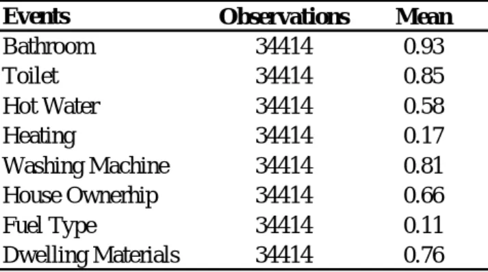
For the descriptive statistics of the selected events see Table 12. 8

including undeclared parts of income. For this purpose, we gradually introduce the under-reported income and the cost of time in the estimations. The simple reason is that we hold the monetary incomes as a touchstone to better clarify its importance for the poor with respect to income data by including the under-reported parts of the self-employed and wage earners' income.

An important decision in the construction of a multidimensional index is the selection of the relative weights for different dimensions. In this paper, we have chosen the equal

weighting scheme9. For the first dimension, we constructed a deprivation index following the

methodology procedure explained above. We consider an individual to be deprived in the second dimension if the proportion of the household budget allocated to food is at least 30% greater than the average budget share of the population. This individual is considered deprived in the third dimension if their total income is strictly lower than the 60% of the

median revenue of the population10. The idea is that, once the deprivation status for each of

the three dimensions has been stated, we classify the population in two groups as the poor and not-poor population, according to the number of dimensions in which they are or they are not deprived. That is, an individual is considered poor if he/she is deprived in all or at least two of the dimensions; they are classed as not poor if he/she is deprived in one dimension or when there is no deprivation at all.

2.1. Uni-Dimensional Approach

From this approach, household income is considered the only dimension that allows a measurement of poverty. Therefore, we adopted the “OECD-modified equivalence scale” first proposed by Haagenars et al.(1994) allowing comparability among net incomes of households

of different sizes during determination of their poverty status11. The equivalence scale consists

of different weightings, assigning a value of 1 to the household head, 0.5 to each additional adult member and 0.3 to each child. This scale states that

*

1 0.5( _a 1) 0.3( _a)

n   n   n n (1)

Wheren ,n , a

*

n corresponds to household size, the number of adults and the number of

adult equivalents respectively. Thus, the transformation from simple per capita household

income y_i /n to _i yn*  y_i/n* yields corrected household income by virtue of different

household sizes. By using the OECD equivalence scale, the rule of dividing total population into poor and non-poor is determined by the reference represented by a one-member household and therefore the individual poverty line is equal to 60% of the median revenue of

the population. Thus the household is considered poor if y is strictly lower than 60% of the n*

median revenue of the population. Finally, a synthetic uni-dimensional poverty measure, such as the head count ratio, could be obtained as the proportion of poor households among the population.

9

Different methods have been widely discussed regarding this issue, but none of them has actually given a normative solution to the problem. The point to consider is that any weighting scheme implies a trade-off between the dimensions, and so we have to be careful while interpreting the results.

10

This ratio is determined by OECD estimations. 11

2.2. Informality and Poverty

The common thought is that tax avoidance and insufficient earnings are the main factors

sustaining the underground economy12. Thus, the most common definition used in the

literature refers to an individual being informal if he/she works but does not have social security. Therefore, the incidence of probable participation in marginal activities among wage earners contradicts this perception of informality. Nevertheless, informality depends on whether or not the individuals that engage in black market or unregistered activities draw particular attention among other definitions in the literature. Indeed, complete demand-based estimation of informality provides a direct at individual level based on the estimation results

at individual level13. In this paper, we consider a household to be informal if the following

conditions are satisfied: respecting our estimation constraint, at least one of the estimated wage and self-employment income coefficients is higher than 1, there under declaration of the total income of the household is apparent. This constraint also takes the household which has two sources of income from both activities into consideration.

Once the households whose informal earnings and conditions of poverty have been identified, we proceed to the calculation of the probabilities of working in the informal market conditional on the poverty status of the households. Since one of the objectives of this paper is to analyze the simultaneous relationship between poverty and informality, we use a bivariate probit model that allows for correlated unobserved heterogeneity. The model is specified as follows: *i i i * i n n n n d d d d n n n n y X u y X u





y are the dummy variables indicating nth household’s informality and

poverty status respectively.X_njis the vector of socio-demographic and work-related

characteristics dummy14.

3. Dataset

We combine the monetary and time expenditures into a unique consumption activity at the individual level. We proceed with the matching of these surveys by regression on similar exogenous characteristics in both datasets as age, matrimonial situation, possession of cell phone, home ownership, number of household members, geographical location separately for

head of household and wife15.

More precisely, we estimate 8 types of time use at Time Use Survey (TUS) which are also

compatible with the available data from Household Budget Survey (HBS) as follows:

Food Time (TUS) with Food Expenditures (HBS)

Personal Care and Health Time (TUS) with Personal Care and Health Expenditures (HBS) Housing Time (TUS) with Housing Expenses (HBS)

Clothing Time (TUS) with Clothing Expenditures (HBS) Education Time (TUS) with Education Expenditures (HBS) Transport Time (TUS) with Transport Expenditures (HBS)

12

See Schneider and Enste (2000). 13

For the brief details of the method and the measurement of complete demand system based estimation of informal economy by Aktuna-Gunes et al. (2015) see Appendix III.

14

Descriptive statistics for the selected variables see Appendix II Table 8. 15

Leisure Time (TUS) with Leisure Expenditures (HBS) Other Time (TUS) with Other Expenditures (HBS)

The food Time consists only of cooking because it is not possible to separate eating activity from Personal Care in the time use survey. Care time consists of personal care, commercial-managerial-personal services, helping sick or old household person and eating activity. Housing Time corresponds to household-family care as home care, gardening and pet animal care, replacement of house-constructional work, repairing and administration of household. Clothing Time consists of washing clothes and ironing. Education Time includes study (education) and childcare. Transport Time consists of travel and unspecified time use. Leisure Time corresponds to voluntary work and meetings, social life and entertainment such as culture, resting during holiday, sport activities, hunting, fishing, hobbies and games, mass media like reading, TV/Video, radio and music. Other Time includes employment and labor searching times.

Valuation of time

By taking advantage of the available TUS and HBS data, we are able to choose the opportunity cost method. Two possible opportunity cost methods for the time valuation of consumption can be used: the first method dictates that we impute the wages net of taxes for non-working individuals using the two-step Heckman procedure: supposing that only time use is perfectly exchangeable for non-market and market activities. In this method the first step estimates a probit equation for participation. The natural logarithm of monthly income, age, age-squared, education dummies, urban variables with the explanatory variables of couples, number of children and number of household members are used to predict the underlying wage rate of households that do not work. Thus, in the second stage the opportunity cost of non-market work is estimated as the expected hourly wage rate in the labor market for those men and women not working. The second method refers to sole market substitution which consists of imputing the same hourly rate for all individuals represented in the surveys, namely minimum wage rate for Turkey in the years 2003, 2004, 2005 and 2006.

Given that individuals spend their time in domestic activities and that time has a cost, we consider the total expenditure of the households as the sum of their monetary expenditure plus time spent for each activity. To do so, we choose the methodology of multiplying time values by minimum wages for the working individuals, while we use the opportunity cost of time obtained through the two-step Heckman procedure for the time values of non-working individuals. The opportunity cost may rather be between these two values (see the discussion in Gardes, Starzec, 2014). The purpose of this double recovery is to obtain more accurate total time values for working and non-working individuals and to increase reliability of the following results.

4. Results

In order to show how incomes gathered from informal activities influence the estimated proportion of the population living in poverty, the self-employed with wage earners’ income were extended by means of the imputation of under-reported estimates using a complete

demand model16. Table 3 reports the changes in the proportion of the lower classes measured

by means of a uni- and multidimensional poverty index and in the Gini coefficient for the years between 2003 and 2006, using four categories of income: monetary income, extended monetary income (i.e. informal earnings added monetary incomes), full income (i.e. monetary income plus monetary time values of domestic activities) and extended full income (i.e.

16

monetary incomes plus informal earnings measured through monetary time values of domestic activities). In order to analyze the role of time spent in domestic activity on the

poverty status of households, we calculate full income that allows for net-effect of time cost17.

As expected, earnings gathered from the informal activities lowers the size of the population living in poverty while the time values estimation included reveals an inverse relationship. Even if the difference between declared income and full income is relatively small for multidimensional estimation (3.32 points), uni-dimensional estimations show a great difference among the population living in poverty (13.15 and 19.16 points for per-capita and equivalence scale, respectively). The fact that there exists a great change already tells us that time spent influences the proportion of poor. Therefore, it is interesting to see that informal earnings reduce the poor population except in multidimensional estimation. The reason could simply be the fact that the weight of the earnings from marginal activities has relatively lost its importance within the dimensions defined in a multidimensional index. Uni-dimensional results confirm that higher level deprivation of sources and low- level opportunity cost of time would result in an increase in informal activities because of lack of goods and services is the

necessary components for domestic production to satisfy the needs18. The proportion of poor

decreases owing to informal earnings from 26.06% to 21.70% and 23.68% to 15.70% respectively for per-capita and equivalence scale estimations. It is interesting to note that these changes are quite bigger after having included domestic incomes (from 39.21% to 29.47% and 42.84% to 27.37%).

Table 3: Average Rates of Poverty (2003-2006)

Monetary Income Extended Monetary Income Full Income Extended Full Income Poor (Multidimensional) 22.11% 27.05% 25.43% 27.73% Poor (Unidimensional) PC 26.06% 21.70 % 39.21% 29.47% Poor (Unidimensional) ES 23.68% 15.70 % 42.84 % 27.37%

Regarding the aim of this paper, extended full income could be taken as the best candidate for more accurate reading of poverty and the Gini results. Thus, changes in poverty status and

income inequality for the years from 2003 to 2006 can be separately taken from Table 419.

The highest poverty rate for multidimensional (28.12%) and per-capita based uni-dimensional (30.67%) index also followed by inequality (36.6) for 2005. Equivalence scale uni-dimensional poverty prediction is 30,47% in 2004 and 29,55% in 2005. Therefore, according to TURKSTAT poverty results, even if poverty is decreasing from 28,12% to 17,81%, it is hard to explain why the Gini coefficient of 2006 reaches 40.3.

17

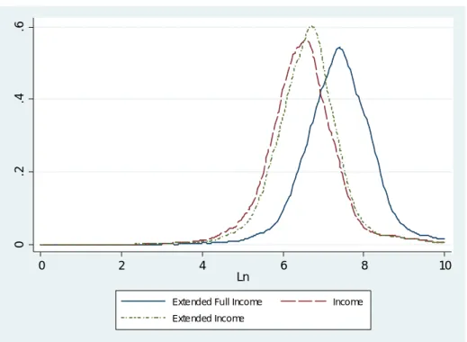
See the Figure 1 on the Appendix I for a picture of log-income kernel densities by monetary, extended monetary and extended full.

18

For size of informal economy estimated by complete demand approach see Table 13 on the Appendix III 19

Table 4: Rate of Poverty and Inequality Using Extended Full Income (2003-2006)

2003 2004 2005 2006

Gini Coefficientsᵇ

(WORLD BANK) 42.2 41.3 41.7 39.7

(*) Complete poverty by food+nonfood (a)By households disponible incomes including informal earnings

estimated through monetary time values of domestic activities (b)By household disposable incomes

20,50% 17,81% Poor (Unidimensional) PC 28,08% 24,78% Poor (Multidimensional) 27,56% 26,53% 28,12% 27,71% 26,97% 29,95% 30,67% 24,16% 36.9 39.1 30,47% 29,55% 28,12% 25,60% 40.3 Gini Coefficientsᵇ (TURKSTAT) 42.0 40.0 38.0 Poor (Unidimensional) ES Poor* (TURKSTAT) Gini Coefficientsᵃ 36.6 35.9

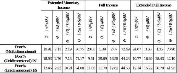
As an additional analysis, Table 5 enables us to follow the percent of change in the proportion of the poor population as it varies across income groups for the years from 2003 to 2006. Keeping declared income as our reference point we can see the distribution of poor for each income after having included the informal earnings and monetary time values. More precisely, “still poor” indicates the households whose poverty status remains the same; “new poor” indicates new poor households where they were not poor before; “new not-poor” consists of the households whose situation has improved relative to their declared income status and, finally, “still-not poor” are the ones who still remain out of poverty after having added additional values into the declared one. The distribution of the households among “new poor” and “new not-poor” shows how earnings from informal activities and monetary time values affect their distribution among the population. Uni-dimensional measurement results indicate an increase (decrease) in new not-poor (new poor) sides for informal earnings (monetary time values) added income. Monetary income results show that the numbers of new poor households, for three poverty estimation, are bigger than the number of new not-poor households when only considering the monetary time values. This result reveals the fact that full incomes obtained by the matching imply relatively higher poverty rates than those computed on monetary incomes for Turkey as an developing country while this could be inverse for developed countries (see Gardes and Starzec, 2014). However, extended full income estimation results, except multidimensional poverty ones, confirm in Turkey's case that informal earnings lower poverty rates.

Table 5: Average changes in poor population compared to declared income (2003-2006) ∆ % S ti ll p o o r ∆ % N e w p o o r ∆ % N ew N o p o o r ∆ % S ti ll N o t-p o o r ∆ % S ti ll p o o r ∆ % N e w p o o r ∆ % N ew N o p o o r ∆ % S ti ll N o t-p o o r ∆ % S ti ll p o o r ∆ % N e w p o o r ∆ % N ew N o p o o r ∆ % S ti ll N o t-p o o r Poor% (Multidimensional) 19.91 7.13 2.19 70.75 20.03 5.39 2.07 72.49 24.07 3.66 1.35 70.90 Poor% (Unidimensional) PC 18.93 2.76 7.13 71.17 9.51 29.69 16.55 44.23 10.77 18.69 28.43 42.10 Poor% (Unidimensional) ES 13.46 2.22 10.21 74.08 11.05 31.78 12.62 44.53 12.14 15.22 30.70 41.93 Extended Monetary

Income Full Income Extended Full Income

In this respect, the question awaiting an answer is how and in which direction changes in relative income and poverty status influence the decision of engaging in marginal activities?

Table 6 represents the results from the bivariate probit model, at the equation set (2), in the

joint estimation of informality and poverty, both for extended monetary income and extended full income in Turkey.

Table 6: Bivariate Probit Coefficients and Marginal Effects

Informality Poverty Informality Poverty

0.224*** -1.358*** -0.133*** 0.321*** -1.381*** -0.131*** (0.019) (0.022) (0.004) (0.019) (0.021) (0.004) -0.024*** 0.002 -0.006*** -0.027*** 0.013*** -0.000*** (0.002) (0.002) (0.000) (0.002) (0.002) (0.000) 0.000*** -0.000 0.000*** 0.000*** -0.000*** 0.000*** (0.000) (0.000) (0.000) (0.000) (0.000) (0.000) 0.128*** 0.104*** 0.011*** 0.074*** 0.099*** 0.013*** (0.018) (0.021) (0.001) (0.018) (0.020) (0.002) 0.282*** -1.351*** -0.046*** 0.188*** -1.053*** -0.066*** (0.020) (0.049) (0.002) (0.020) (0.037) (0.002) 0.056* -2.362*** -0.050*** 0.071** -2.045*** -0.066*** (0.025) (0.195) (0.001) (0.025) (0.127) (0.001) 4.286*** 0.135*** 0.096*** 3.890*** -0.128*** 0.114*** (0.245) (0.027) (0.005) (0.238) (0.026) (0.005) 3.932*** -0.112*** 0.069*** 4.121*** -0.288*** 0.101*** (0.246) (0.028) (0.003) (0.239) (0.026) (0.004) 0.206*** -0.680*** -0.026*** 0.227*** -0.517*** -0.027*** (0.031) (0.034) (0.001) (0.031) (0.033) (0.002) 0.030 -0.387*** -0.027*** -0.013 -0.221*** -0.021*** (0.020) (0.024) (0.002) (0.020) (0.023) (0.002) 0.222*** -0.320*** -0.012*** 0.306*** -0.271*** -0.008*** (0.061) (0.061) (0.002) (0.061) (0.058) (0.004) - -0.553*** -0.046*** - -0.585*** -0.064*** (0.020) (0.002) (0.019) (0.003) -3.898*** 0.772*** -3.815*** 0.969*** (0.246) (0.047) (0.240) (0.046) (0.013) Marginal Effects (dy/dx)=0.044 Urban Age Age Squared Working Females Secondary Education Error terms correlation rho ***p<0.01, **p<0.05, *p<0.1 Monoparental Family Superior Education

Couple with Children

Couple without Children

Constant Wage Earners

Wald test of rho=0

Dwelling Materials Self Employment

Variables

Ext. Monetary Income Marginal Effects (dy/dx)=0.030

Ext. Full Income

chi2(1)=487.126, Prob > chi2 = 0.000 chi2(1)=948.932, Prob > chi2 = 0.000 -0.317***

(0.014)

Our estimations confirm that despite controlling for many relevant variables, informality is

highly correlated with poverty20. After controlling for unobserved heterogeneity, we can see

that individuals living in urban areas have a lower risk of living in poverty than those living in rural areas. This result is coherent with TURKSTAT rates in Table 1. Therefore, monetary time value added income estimation shows that they are also much more inclined to work in the informal sector, probably due to the difficulties that they face when looking for a job in the labour market. Age, entered linearly, has a negative effect on both poverty and jobs in the informal sector, reflecting more conservative behavior from older workers who may be less willing to participate in entrepreneurial adventures.

It is also interesting to see how working females are more likely to be in poverty and work in the informal sector at the same time. On the one hand, this may possibly be because there is no other immediate option and it is better for them to work even under bad conditions than not work at all. Essentially, they have no other choice than to work informally. Level of education decreases the probability of living in poverty and increases at a diminishing rate of working in the informal sector with respect to those individuals that have just had primary school or no education at all; reinforcing the idea that mostly poor households work in the informal labor market. Furthermore, a similar case of living in poverty and suffering the risk of engaging in informal activity exists also for self-employed and wage earners. The question desiring an answer is why these individuals are living in poverty and are subject to a high level of probability of participating in informal activities. In fact, it would be expected that participating in informal and domestic activities can also be correlated with any peer effect among and between the social groups. Thus, this tendency may result from psychological factors associated with habit formation and social interdependencies based on relative income

concerns21. Household satisfaction seems to be influenced by the given consumption level

also depending on its relative magnitude in the social group. This motivation justifies Duesenberry’s (1948, 1949) assumptions on consumption decisions which are motivated by

“relative” consumption22 and which has two dimensions: first, these households would have a

desire to be close to the consumption structure of the upper bound (rich households) within their reference group. This is the inner relation between the individual and his/her reference group. Second, motivation would be, respecting Duessenberry’s idea of the socio-psychological difficulties due to reducing the given expenditure scheme of households, a desire to be away from the consumption structure of the individuals who are included in the upper bound of the lower reference group. This is the external relation between the individual and other reference groups. In other words, the poorest individuals in the poor population would want to be close to the consumption structure of the relatively richer poor in their reference group but not to that of the poorest ones in the lower groups. The high level income distribution of equalities, especially in developing economies, would promote this motivation. Therefore, such a phenomenon justifies the existence of high level luxury goods-buying in these countries.

Regarding the household structure, couples with or without children are more inclined to work in the informal market but less likely to be in poverty, as are monoparental families. In

20

In our estimation, the results for the correlation coefficient of the error terms, which is statistically significant for both estimation; and the results for the Wald statistics, which rejects the null hypothesis that= 0. So we can conclude, that the error terms of the equations jointly estimated varies together.

21

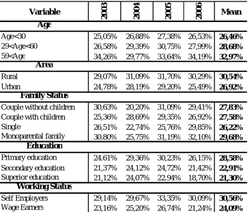
Sub-population poverty rates as for the categories of age, area, education, family and working status see Tables 9-11.

22

According to Duesenberry (1948) the strength of any individual’s desire to increase his consumption expenditure is a function of the ratio of his expenditure to some weighted average of the expenditures of others with whom he comes into contact.

fact, having two salaries reduces the chances of being poor; furthermore, if one of the salaries is drawn from the formal sector, the couple may be more inclined to entrepreneurial activities. Lastly, the household, especially the one that devotes a large amount of time in domestic activities tend to have lifestyles favoring more spending on accommodation. Thus, we choose accommodation as a control variable that can be used as a proxy of the decision between marginal activities. Nevertheless, domestic activity plays an important role. Indeed, it is interesting to see that people whose accommodations are sound are less likely to be poor and enjoy domestic activity.

5. Conclusion

This study uses microeconomic data from Time Use surveys and Family Expenditure surveys in order to examine the effect of incomes gathered from informal and domestic activities on the proportion of the population living in poverty and income distribution inequalities in Turkey. The results show that extended monetary and extended full incomes differ from the declared monetary ones in a significant way, suggesting that the incorporation of incomes from marginal activities through the valuation of time can have a relevant impact on the determination of the proportion of poor and the Gini coefficient. Being engaged in informal activities causes decreases in the proportion of poor and inequalities of income distribution while including monetary values of time added to income implies a higher level of poverty. The Gini coefficient estimation results indicate that including monetary time values of domestic activities increases the inequality parallel to that of the poor population.

As a complementary analysis, in order to analyze the simultaneous relationship between poverty and informality, we use a bivariate probit model that allows for correlated unobserved heterogeneity. By taking advantage of knowing the individuals who participating in informal activities and their poverty status before and after adding informal earnings, we are able to measure the probabilities of participating in informal activities for the poor population. Finally, the monetary time use values (i.e. domestic activities) of households allow us not only to know household’s informal economy participation decision but also gives us an important information about their poverty status. The results show that extended full incomes increase the joint probability of being in poor and work in the informal sector.

References

ADAMS, R. H. and JOHN, P., (2001), “Holding the Line: Poverty Reduction in the Middle East and North Africa, 1970-2000”, Poverty Reduction Group, World Bank, Washington D.C. AKDER, H., (1999), “Türkiye’de Kirsal Yoksullugun Boyutlari”, Technical Report, World Bank.

ARAN, A. M., DEMIR, S., SARICA, O., YAZICI, H., (2010),“Poverty and Inequality Changes in Turkey (2003–2006)”, Working Paper, State Planning Organization and World Bank Welfare and Social Policy Analytical Work Program, Ankara

AKTUNA-GUNES, A.T., STARZEC, C., GARDES, F., (2014), “ Une évaluation de la taille de l'économie informelle par un système complet de demande estimé sur données monétaires

et temporelles”, Revue économique, No : 65-4, pp.567 - 589.

AKTUNA-GUNES, A.T., GARDES, F., STARZEC, C., (2015), “ The Size of Informal

Economy and Demand Elasticity Estimates Using Full Price Approach: A Case Study for Turkey ”, Documents de Travail du Centre d’Economie de la Sorbonne (CES).

AKTUNA-GUNES, A.T. and CANELAS C., (2013), “A Multidimensional Perspective of Poverty, and its Relation with the Informal Labor Market: An Application to Ecuadorian and Turkish Data” Documents de Travail du Centre d’Economie de la Sorbonne (CES).

ATKISON, A.B., RAINWATER, L., SMEEDING, T. M., (1995), Income Distribution in

OECD Countries. Evidence from the Luxembourg Income Study,OECD Social Policy Studies,

No. 18, Paris.

BIBI, S., (2005), “Measuring Poverty in a Multidimensional Perspective: A Review of Literature”, Working Papers, PEP-PMMA.

BUGRA, A. and KEYDER, C., (2003), “Yeni Yoksulluk ve Türkiye’nin Degisen Refah Rejimi” Technical Repor for UNDP.

BUGRA, A. and KEYDER, C., (2006), “The Turkish welfare regime in transformation”,

Journal of European Social Policy,C,16/3, p.211–228.

CAGLAYAN, E. and DAYIOGLU, T., (2011), “Comparing the Parametric and Semiparametric Logit Models: Household Poverty in Turkey”, International Journal of

Economics and Finance, 3/5, p.197–207.

CHAI A. and MONETA A., (2010), “Retrospectives: Engel curves.”, J Econ Perspect, no 24-1, pp:225-240

DEATON, A., (2000), The analysis of household surveys. A microeconometric approach to development policy, Baltimore and London, John Hopkins University Press, 3rd ed.

DELHAUSSE, B., LUTTGENS, A., PERELMAN, S., (1993), “Comparing measures of poverty and relative deprivation: An example for Belgium”, Journal of Population

Economics. 6 :83-102.

DESAI, M. and SHAH, A., (1988),“An econometric approach to the measurement of poverty.” Oxford Econ Pap. 40:505-522

DUESENBERRY, J.S., (1948), “Income - Consumption Relations and Their Implications,” in Lloyd Metzler et al., Income, Employment and Public Policy, New York: W.W.Norton & Company, Inc.

DUESENBERRY, J.S., (1949), Income, Saving and the Theory of Consumption Behavior, Cambridge, Mass.: Harvard University Press.

DUMANLU, R., (1996),“Türkiye’de Yoksulluk Sorunu ve Boyutları”, Yoksullukla Mücadele Stratejileri, Hak-İş Konfederasyonu Yayınları, Ankara.

ERDOGAN, G., (1996),“Türkiye’de bölge ayriminda yoksulluk siniri üzerine bir çalisma” Thesis for Turkish Statistical Institute, Ankara.

GARDES, F., and STARZEC, C., (2014), “Individual prices and household’s size: a restatement of equivalence scales using time and monetary expenditures combined”, Working

Paper, Centre d’Economie de la Sorbonne (CES).

GULOGLU, T., AYDIN, K., GULOGLU. F.K., (2012), “Relative Poverty in Turkey Between 1994 and 2006”, Economics and Management¸ 17/1, p. 163-175.

HAGENAARS, A., K. de VOS and ZAIDI, M.A., (1994), Poverty Statistics in the Late

1980s: Research Based on Micro-data, Official Publications of the European Communities.

Luxembourg.

ILKKARACAN, A.I. and GUNDUZ, U., (2009), “Time-use, the Value of Non-Market Production and its Interactions with the Market Sector: The Case of Turkey”, Paper presented at International Conference on Inequalities and Development in the Mediterranean Countries,

Mimeo

KLASEN, S., (2000), “Measuring Poverty and Deprivation in South Africa”, Review of

Income and Wealth, 46, 33-58.

LANGLOIS, S. and GARDES. F., (2003), “La pauvreté en France et au Québec : une comparaison à l'aide de l'indice multidimensionnel de pauvreté-richesse”,Santé, société et

solidarité ,1, p. 181-189.

MUELBAUER, J., (1980), “The Estimation of the Prais-Houthakker Model of Equivalence Scales”, Econometrica, Econometric Society, 48/1, p.153–76.

OECD, (2009), “Poverty reduction and social development: Is Informal Normal? Towards More and Better Jobs in Developing Countries?”,Overview: Data on Informal Employment

and Self-Employment.

OGUZLAR, A., (2006), “Diskriminant Analiz Yoluyla Hanehalki Türünün ve Kir-Kent Ayrimlarinin Degerlendirilmesi”, Akdeniz Universitesi I.I.B.F. Dergisi, 11, p.70–84.

PAMUK, M., (2000), “Kırsal Yerlerde Yoksulluk”, DİE İşgücü Piyasaları Analizleri”, Report for Turkish Statistical Institute, Ankara.

PRADHAN, M. and MARTIN, R., (2000), “Measuring Poverty using Qualitative Perceptions of Consumption Adequacy.”, Review of Economics and Statistics, 82, p:462–71.

PRAIS, S.J. and HOUTHAKKER, H.S., (1955), The Analysis of Family Budgets, Cambridge University Press, Cambridge, 2nd ed.-1972

SADOULET, E., and JANVRY, A. (1995), Quantitative Development Policy Analysis, Baltimore and London, John Hopkins University Press.

SAHN, D. and STIFEL, D., (2001), “Exploring Alternative Measures of Welfare in the Absence of Expenditure Data”, Cornell University.

SCHNEIDER, F. and ENSTE D., (2000),“Shadow Economies: size, causes and consequences” Journal of Economic Literature, 38, p.77-114.

SEKER, S.D. and JENKINS,. S.P., (2013), “Poverty Trends in Turkey”, Working Paper, IZA DP No. 7823.

SEN, A., (1985). The Standards of Living, Cambridge University Press.

SMEEDING, T., SAUNDERS, P., CODER, J., JENKINS, S.P., FRITZELL, J., HAGENAARS, A., et al. (1993), “Poverty, inequality and family living standards impacts across seven nations: the effect of non-cash subsidies for health, education and housing”,

Review of Income and Wealth, 39, 229-256.

TOWNSEND, P., (1979), Poverty in the United Kingdom, London, Allen Lane and Penguin Books.

TURKISH STATISTICAL INSTITUTE (2006,2005,2004,2003), Household Budget Survey TURKISH STATISTICAL INSTITUTE (2006), Time Use Survey

YALMAN, G.L., (2006), “Güneydogu Anadolu’da yoksullugu azaltmak için uygulanan programlarin bir degerlendirmesi”, Technical Report for TESEV-IPC.

Appendix I

Table 7: Income and Expenditure Descriptive Statistics

Variable N Mean Std Dev Minimum Maximum

Food 34414 0.3139 0.1528 0 1.0000

Personal Care(with Health) 34414 0.0782 0.0756 0 0.8362

Housing 34414 0.3336 0.1398 0 1.0000

Clothing 34414 0.0586 0.0703 0 0.5893

Education 34414 0.0117 0.0465 0 0.8323

Transport 34414 0.0799 0.0982 0 0.8723

Leisure 34414 0.0586 0.0570 0 0.8859

Variable N Mean Std Dev Minimum Maximum

Food 34414 0.1600 0.0744 0.0154 0.7459

Personal Care(with Health) 34414 0.1441 0.0427 0.0071 0.6846 Housing 34414 0.1716 0.0896 0.0261 0.9040 Clothing 34414 0.0327 0.0375 0.0004 0.4431 Education 34414 0.0097 0.0282 0.0001 0.7469 Transport 34414 0.0825 0.0619 0.0070 0.7838 Leisure 34414 0.2678 0.0796 0.0177 0.8674 Variable N Mean Std Dev Minimum Maximum Self employment / Total Income 34414 0.2682 0.4073 0 1.0000 Wage / Total Income 34414 0.4689 0.4225 0 1.0000 Variable N Mean Std Dev Minimum Maximum Self employment / Total Income 34414 0.2906 0.4235 0 1,1278 Wage / Total Income 34414 0.5433 0.4734 0 1.1219 Variable N Mean Std Dev Minimum Maximum Self employment / Total Income 34414 0.2956 0.4287 0 1.1352 Wage / Total Income 34414 0.5446 0.4746 0 1.1423 Budget Shares MONETARY EXPENDITURES FULL EXPENDITURES Budget Shares EXTENDED FULL Household income share : EXTENDED MONETARY Household income share : Household income share : MONETARY

Table 8: Bivariate Probit Model Descriptive Statistics

Variable Obs. Mean Std. Dev. Min Max

%Urban households 34414 0,665 0,472 0 1 Age 34414 38.01 17.19 3 99 % Male HH 34414 0,952 0,214 0 1 % Female HH 34414 0,342 0,474 0 1 Primary Education 34414 0,703 0,457 0 1 Secondary Education 34414 0,189 0,392 0 1 Superior Education 34414 0,108 0,310 0 1 Self Employment 34414 0,364 0,481 0 1 Wage Earners 34414 0,600 0,489 0 1

Others Earners(without working) 34414 0,756 0,429 0 1

Number of children 34414 1,407 1,437 0 13

Households Size 34414 4,333 1,966 1 23

Couple without Children 34414 0,103 0,304 0 1

Couple with Children 34414 0,668 0,471 0 1

Single 34414 0,020 0,140 0 1

Monoparental Family 34414 0,024 0,153 0 1

Dwelling Materials 34414 0,762 0,425 0 1

Table 9: Poor (Multidimensional)(in%)

Variable 2 0 0 3 2 0 0 4 2 0 0 5 2 0 0 6 Mean Age Age<30 31,67% 28,48% 23,74% 28,68% 28,14% 29<Age<60 24,29% 26,50% 27,13% 26,94% 26,22% 59<Age 44,39% 28,81% 39,71% 42,36% 38,82% Area Rural 31,80% 32,60% 31,98% 34,12% 32,63% Urban 34,89% 28,03% 36,50% 34,86% 33,57% Family Status

Couple without children 35,25% 21,53% 37,23% 39,47% 33,37%

Couple with children 23,46% 26,35% 26,69% 27,65% 26,04%

Single 35,81% 22,44% 40,90% 37,31% 34,12% Monoparental family 39,44% 23,56% 43,01% 46,91% 38,23% Education Primary education 29,56% 26,20% 28,77% 28,85% 28,35% Secondary education 21,90% 24,25% 24,62% 26,63% 24,35% Superior education 19,74% 35,92% 47,46% 45,13% 37,06% Working Status Self Employers 33,24% 29,78% 34,59% 47,51% 36,28% Wage Earners 29,83% 28,59% 23,31% 26,59% 27,08%

Table 10: Poor (Unidimensional-PC)(in%) Variable 2 0 0 3 2 0 0 4 2 0 0 5 2 0 0 6 Mean Age Age<30 25,05% 26,88% 27,38% 26,53% 26,46% 29<Age<60 26,58% 29,39% 30,75% 27,99% 28,68% 59<Age 34,26% 29,77% 33,64% 34,19% 32,97% Area Rural 29,07% 31,09% 31,70% 30,29% 30,54% Urban 24,78% 28,19% 29,20% 25,49% 26,92% Family Status

Couple without children 30,63% 20,20% 31,09% 29,41% 27,83%

Couple with children 25,36% 28,69% 29,35% 26,92% 27,58%

Single 26,51% 22,74% 25,76% 29,85% 26,22% Monoparental family 30.80% 25,75% 31,19% 32,10% 29,68% Education Primary education 24.61% 29,36% 30,23% 26,15% 28,58% Secondary education 21,37% 24,12% 24,72% 21,42% 22,91% Superior education 21,12% 24,07% 22.94% 18,70% 21,30% Working Status Self Employers 29,14% 29,67% 33,35% 30,09% 30,56% Wage Earners 23,16% 25,20% 26,74% 21,24% 24,09%

Table 11: Poor (Unidimensional ES)(in %) Variable 2 0 0 3 2 0 0 4 2 0 0 5 2 0 0 6 Mean Age Age<30 21,12% 24,80% 26,17% 22,39% 23,62% 29<Age<60 23,47% 29,86% 29,75% 24,58% 26,92% 59<Age 35,19% 23,35% 36,45% 31,83% 31,71% Area Rural 25,68% 31,61% 31,08% 25,31% 28,42% Urban 21,62% 28,87% 28,02% 22,31% 25,21% Family Status

Couple without children 30,42% 20,24% 27,64% 29,42% 26,93%

Couple with children 22,27% 29,03% 28,75% 24,59% 26,16%

Single 27,44% 23,03% 30,30% 31,34% 28,03% Monoparental family 28,72% 24,38% 31,18% 33,33% 29,40% Education Primary education 21,11% 31,10% 28,87% 23,79% 26,22% Secondary education 17,74% 24,92% 23,62% 19,15% 21,36% Superior education 15.63% 25,80% 22,24% 15,77% 21,27% Working Status Self Employers 28,82% 29,23% 32,70% 27,71% 29,62% Wage Earners 19,81% 26,21% 24,86% 19,70% 22,65%

Figure 1: Kernel Density Distribution of Incomes 0 .2 .4 .6 0 2 4 6 8 10 Ln

Exte nded Full Income Income Exte nded Income

Appendix II Deprivation Index

Following Desai and Shah (1988), the index of relative deprivation Dj corresponding to the household j, is estimated as 1 I _ˆ j i ij i D I

 

_

where each I corresponds to a consumption event, ˆ to the estimated distance between the _ij

household and the community experience for the ith event, and  the weight of the i_i th event.

In this article, following Delhausse et al., ˆ was redefined on the basis of probabilities as : _ij

ˆ _{(ˆ )}

ij ij i







where  is a central probability measure, and _i  is the estimated probability for ˆ_ij

household j, to experiment the ith event. Also, (1

_

order to normalize index magnitudes. Finally, it is assumed that each experience has a specific

weight _i _iin order to take prevalent social norms into consideration.

The estimation of probabilities was carried out by logit regression of household experiences, indicated by dichotomous variables, on several variables representing socio-demographic characteristics.

Table 12: List of Selected Events

Events Observations Mean

Bathroom 34414 0.93 Toilet 34414 0.85 Hot Water 34414 0.58 Heating 34414 0.17 Washing Machine 34414 0.81 House Ownerhip 34414 0.66 Fuel Type 34414 0.11 Dwelling Materials 34414 0.76 Appendix III

Let true income (Y*) be separated into three sources denoted a, s, r which respectively correspond to other income sources, wages and self-employment income. The total reported (true) income is supposed to be a weighted sum of these three sources:

(5)

This equation implies that the true income must be equal to the sum of the observed

income (Ya, Ys, Yr) multiplied by their corresponding factor (θa, θs, θr), where we suppose θm ≥

1 (i.e., under reporting) and θa = 1 (correct observation of the other incomes). Such hypothesis

allows us to estimate the under reporting part of self-employers and wage workers23 under the

assumption that they may also save certain parts of their under reported income to finance durable and non-durable goods purchases. It allows us to calculate the size of the underground economy and the saving tendencies with respect to the under reporting part of declared

incomes by an estimation of θr and θs. In order to impose the constraint on the θr and θs

parameter (θr,s ≥ 1), Fortin et. al (2009) propose to express it by (1+ek) where k is a parameter

estimated by the model. Additionally, we suppose that the true value of self-employment and

wage income (Yr* and Ys*) can respectively be then denoted as (1+ek)*Yr and (1+el)*Ys

where l represents the parameter as an under reported part estimated for wage workers.

Finally, we could determine the sum of each source of income as a ratio of the reported

total income: ym = Ym/Y, where Y is the sum of other sources as fees, government transfers,

etc. as well as wages and self-employment incomes. Following the model proposed by Aktuna-Gunes et al. (2014), we consider all goods and services with full price values in the estimation model as follows:

, 1 , , , , 3 2 ( )n ln Y ln( ) ln Y ln( ) log ih i ij jh in r s i h m m i h m m i ih ih j n m a s r m a s r Z y y y e w                                   (6) 23

This is a necessary constraint. According to the research conducted by Republic of Turkey Social Security Institution in 2011, 75 of every 100 wage workers, declared as minimum wage, is lower than their real wage rate. Therefore, the part of the disposable income of regular employee represents 42.8%, 54.5%, 57%, 58.9% in total GDP respectively for the years between 2003–2006

* , , Y_{h m}Y_mh m a s r   

_

where w,  , Z, j and i represent respectively the budget share the full prices and the

household characteristics vector (which allows us to take into account the heterogeneity of preferences). We cannot expect that the individuals from different social groups have the same reaction in consumption and saving choices with respect to the different types of incomes especially when there is uncertainty about these revenues. In accordance with Lyssiotou et al. (2004), we thus introduce in each equation linearly the powers of incomes r

and s (∑3n=1 λin(yr,s)n ) in order to reflect the relative importance of self-employed and wage

incomes in the total household’s income. The purpose of this expression is to diminish any possible confusion between consumption heterogeneity and the phenomenon of the under-reported part of self-employed and wage earners' income.

Table 13: The Size of Informal Economy with Full Prices for the Years between 2003 and

2006 (In %)

Year Parameters k, v

(Std. Err) 2003 2004 2005 2006 Average

Size of informal economy for monetary expenditure estimation (SE)ᵃ 1.58 *** _(0.316) 39,64% 41,96% 40,89% 33,76% 39,07%

Size of informal economy for monetary expenditure estimation (WE)ᵇ 0.48**

(0.149) 24,34% 26,16% 27,36% 28,27% 26,53% Size of informal economy for full expenditure estimation (SE)ᵃ 1.91 **

(0.852) 47,92% 50,73% 49,43% 40,82% 47,22% Size of informal economy for full expenditure estimation (WE)ᵇ 0.58*** _(0.248) 29,41% 31,61% 33,06% 34,16% 32,06% ***p<0.01, **p<0.05, *p<0.1

a: Self Employers; b: Wage Earners