HAL Id: halshs-00966364
https://halshs.archives-ouvertes.fr/halshs-00966364
Preprint submitted on 28 Mar 2014HAL is a multi-disciplinary open access archive for the deposit and dissemination of sci-entific research documents, whether they are pub-lished or not. The documents may come from teaching and research institutions in France or abroad, or from public or private research centers.
L’archive ouverte pluridisciplinaire HAL, est destinée au dépôt et à la diffusion de documents scientifiques de niveau recherche, publiés ou non, émanant des établissements d’enseignement et de recherche français ou étrangers, des laboratoires publics ou privés.
Trade Liberalization And Poverty Dynamics in Vietnam
2002-2006
Barbara Coello, Madior Fall, Akiko Suwa-Eisenmann
To cite this version:
Barbara Coello, Madior Fall, Akiko Suwa-Eisenmann. Trade Liberalization And Poverty Dynamics in Vietnam 2002-2006. 2010. �halshs-00966364�
Trade Liberalization
And Poverty Dynamics
in Vietnam 2002-2006
Barbara COELLO
World Bank Madior FALL Afristat
Paris School of Economics INRA
Akiko SUWA-EISEMANN Paris School of Economics
INRA
June 2010
G-MonD
Working Paper n°11
1
Trade liberalization and poverty dynamics
in Vietnam 2002-2006
Barbara Coello, the World Bank
Madior Fall, Afristat and Paris School of Economics-INRA
Akiko Suwa-Eisenmann, Paris School of Economics-INRA
1June 6, 2010
1
Paris School of Economics, 48 Boulevard Jourdan, 75014 Paris. France [email protected]. This work was undertaken while Barbara Coello was in the doctoral program at PSE, under contract RCH 029-2005 with Agence Française de Développement.
We are very grateful to Loren Brandt, Jean-Pierre Cling, Lionel Fontagné, Jean-Pierre Laffargue,Brian McCraig, Marta Menendez, Nina Pavcnik, Martin Ravallion, Qy-Toan Do, Marie-Cécile Thirion and Dominique Van de Walle.
2
Trade liberalization and poverty dynamics
in Vietnam 2002-2006
Abstract
This paper shows the evolution of poverty in Vietnam during the deepening of trade liberalization and examines the impact of trade-related variables at the household level. The study is based on a panel dataset of households followed in 2002, 2004 and 2006. Trade-related variables at the household level are defined as the household specialization in terms of production and employment with respect to the type of jobs (wage earners or self-employed) and sectors (import-competing or exported manufactured goods, services, and in agriculture, rice, exported, subsistence and import-competing crops). For the poor, besides the expected positive impact of working in an export-related sector (in industry and in agriculture), diversification in self-employed non-farm activities appears to have been efficient at alleviating poverty. Moreover, the import-competing sectors (in industry and in agriculture) play also a positive role in poverty alleviation. The latter channel could be hindered in the near future, as Vietnam is now in the process of decreasing its import protection
.
JEL Classification numbers: C23;I32;O19;O53
3
1. Introduction
The impact of trade liberalization on household welfare has been widely debated. Studies based on cross-country data have shown a positive impact of trade on growth and hence, on poverty (Dollar and Kraay, 2004). However, micro evidence at the household level shows that trade creates losers as well as winners (Goldberg and Pavcnik 2007). In this paper we focus on poverty dynamics in an Asian country, Vietnam.
Vietnam has been often cited as an example of a successful economic liberalization and trade opening which managed to improve household welfare. Poverty dropped sharply, from 58% of the population at the start of economic reform to a mere 16% en 2006 (Glewwe, Gragnolati and Zaman 2002). Meanwhile, inequality either decreased or remained stable. Vietnamese experience in that respect contrasts with that of China where inequality increased during economic reform (Ravallion 2010).
Poverty is studied in this paper in a micro-economic perspective, at the household level. A household is deemed poor if his consumption per capita is below a minimum level. Studies on poverty are often based on cross sections and focus mostly on one indicator, the share of poor in the population (the headcount). Here we look not only at the headcount but also at how far is a given household below the minimum level, namely the severity of poverty. Actually, we show that the severity of poverty increased for some household categories between 2002 and 2006, despite the general drop in the share of total population below the poverty line. Indeed, the distribution among the poor themselves matters. Households who remained poor after 2002 are far below the poverty line and could not easily improve their living conditions.
Theoretical analyses have shown the importance of looking at the dynamics of poverty. Recent empirical surveys on poverty have stressed the importance of following poverty mobility with longitudinal data (Dercon and Shapiro, 2009; see also Fall and Menendez, 2009, for developed countries). It matters indeed to know who escape poverty and who is staying behind, who is vulnerable to transient poverty spells or is subject to chronic poverty, especially in times of overall economic reform.
We take stock from the existence of repeated household surveys in Vietnam, where a subset of households were interviewed three times, in 2002, 2004 and 2006. Thus, we are able to follow these households over time and relate their fate to change in contextual trade-related changes.
Previous papers looked at poverty in Vietnam during the 90s, using another available panel dataset which stretched over 1993-1998. We update the results of these papers for the period 2002-2006. The bulk of domestic and export liberalization occurred in the 90s and deepened in the 2000s: textile industry soared, major trade agreements were signed and implemented, beginning with the free trade
4
agreement with the United-States in 2001, and foreign direct investment (FDI) flew in. On the import side, liberalization started only after 2000. This policy turn can matter on income distribution for households up to then protected from foreign competition.We characterize extensively the nature of the contextual trade-related variables that influence households. We distinguish first between self-employed and wage earners and we take also into account the fact that in a developing country such as Vietnam, an individual might have multiple activities and work part-time for wage, while also being self-employed. We distinguish the trade orientation of the sector one is working in: export industry, import-competing industry, and non-traded services. Moreover, based on a previous paper on rural households (Coello 2009), we extend this characterization to farmers. We thus define agricultural households depending on the market orientation of the crops they produce: import-competing, non-traded crops (subsistence) or exported crops. The latter group is further divided between the main export crops (coffee, pepper, cashew nuts, and tea) and other cash crops. Rice producers appear as a separate category, as rice, which is the main staple in Vietnam, is exported, imported and locally consumed either on the farm or sold on domestic markets.
We relate the change in real per capita expenditure between 2002 and 2006 to household characteristics, location and farm characteristics and change in the trade-related contextual variables. We then consider specifically as a dependent variable the change in expenditures for households who were poor in 2002. We perform different types of robustness checks. First, we redo the first regression not with the change in the contextual variables between 2002 and 2006, but with their level in 2002. Second, we consider an alternative definition of job categories. Third, we use a multinomial logit on poverty transitions, and we consider in particular, households who were poor in 2002 and escaped from poverty since then.
We find that in Vietnam, new opportunities that improved the welfare of the general population did not systematically reach the poor. For instance, the extension of formal wage earnings and the rise in exports, both in industry and in agriculture, as well as the growth of the services sector improved the living condition of the population in general. However, those who were poor in 2002 were mostly rural and depending on agriculture. Hence, cash crops exports were important indeed for them, as well as new opportunities in self-employed non agricultural activities, and they also kept relying on import-competing crops.
2. Two decades of trade liberalization in Vietnam and its likely impact on household
welfare and poverty
The two steps of trade liberalization
Economic reform in Vietnam started in 1986 (the Doi Moi). The process involved domestic liberalization, from a state economy to a market oriented one. Agriculture was promoted through
5
decollectivization and a land reform (Gallup (2003), Brandt and Benjamin (2002), Minot, and Goletti (2000) Edmonds and Pavcnik (2004).On the trade side, Vietnam gradually turned from an import-substitution policy to an export-promoting policy. Liberalization occurred in two steps. During the first period, the 1990s, multiple exchange rates were unified, enterprises were allowed to export outside the socialist countries of the Council of Mutual Economic Assistance (CMEA), pro-FDI legislation was passed and a number of regional and multilateral agreements were negotiated. Vietnam joined the ASEAN, the AFTA and became a member of the GATT in 1995. Export quotas were eliminated in 1995 for all commodities except rice. In the process of accession to the WTO, import quotas were gradually transferred into tariffs, except for eight categories of goods (Athukorala 2002; Auffret 2003). The transfer from Non tariff barriers to tariff protection resulted actually in an increase in the level of tariffs, even though some important inputs, such as fertilizer, or later, industrial machinery, experienced a drop in tariffs. Overall, during the nineties, import tariffs and to a lesser extent export tax, remained complex and subject to temporary rises; import protection of final goods remained at a high level (Figure 1). As a consequence, during this first period, the effects of openness mostly occurred through exports (Niimi et al. 2007, Justino and al. 2008, Coello 2008).
The signing in 2001 of the bilateral trade agreement with the United States can be seen as the start of the second stage of liberalization. Import protection on final goods started to decline, leading to a competition between domestic and imported products. This trend was further exacerbated with the entry of Vietnam into the WTO in 2007. As a result, the share of trade in Vietnam GDP boomed in the 2000s. Exports and imports of goods and services represented respectively 55% and 57% of GDP in 2000, 76% and 90% in 2006. FDI also rose substantially, after the requirement of a joint-venture with domestic investors was suppressed after 2000.
Trade liberalization and households: the different channels
In this paper, we focus on the micro linkages going from trade liberalization to households’ income (surveyed in Hertel and Reimer (2005) and Goldberg and Pavcnik (2004)). We do not consider macro linkages that would go through the overall stabilization of the economy and growth. We follow and precise the framework described in Winters, McCulloch and Cirera (2001). Trade liberalization hits households through direct and indirect effects. Direct effects go through products (their prices, quantities and number of varieties) and factors markets (wages, employment, and new job opportunities). The indirect effects (not examined in this paper) concern changes in government revenues and social spending. The general framework has been widely applied, and in particular to Vietnam during the 90s (Justino, Litchfield and Pham, 2008; Niimi, Vasudeva-Dutta and Winters,
6
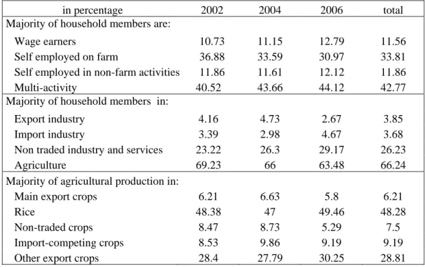
2007). In the following, we precise this framework in the case of Vietnam during the second stage of trade liberalization.In the case of Vietnam, the economic structure has changed indeed, but more on the production side than on employment. Despite a rise of industry share in GDP from 23% in 2000 to 40% in 2006, the share of industry in total employment remained barely the same, at around 20%. Even with stable employment, factor earnings might have increased in industry. However, we must add here a caveat: households where a majority of members are working in export industries count less than 4% of the dataset, almost as much as households involved in import-competing industries. Most households (66%) are dependent on agriculture, even if this proportion is decreasing over time. Last, around one household out of four is dependent on (non-traded) services, and this share is increasing.2
Domestic and trade liberalizations might also have altered the job pattern, namely the share of formal wage jobs (McCraig 2009). Unfortunately, we do not know if a job is informal or not. However we know in the dataset we will be using in this paper, that a mere 11% of households have a majority of their members working for wages (an average household counts four adult members). This proportion increases slightly between 2002 and 2006 (table 1). Most households have a majority of their members in self-employed farm activities (33%), even if this proportion is decreasing over time. Households with members self-employed in non-farm activities are as numerous as households with wage earners. Last, over 40% of households members engage in multi-activity jobs and this proportion is increasing over time. Typically, this might concern farmers diversifying their activities with petty trading or transport on a part-time basis. Thus, the evolution of self-employment as well as multiple-activity jobs matters for households, and as we will see, more for the poorest.
A particularly significant crop in Vietnam is rice. Rice is the main staple and accounts for more than 68% of the average calories intake in 2006 and even 78% for the poor (Glewwe and Vu, 2008). Rice in Vietnam has a special status, as it is at the same time, exported and imported, sold on domestic market and retained for own consumption by rural households. Besides rice, trade liberalization has promoted export crops such as coffee, pepper or cashew (labeled hereafter, the “main export crops”) and farmers who could afford it took advantage of these new opportunities by switching their crop mix (Coello 2009). For instance, many farmers in Central Highlands have switched to coffee and more recently to cashew (Benjamin and Brandt, 2002, Benjamin, Brandt and Coello 2009). However, half of total agricultural households still live mostly from rice production, 6% from the main export crops, and 29% from other export crops. In addition, 9% of these households are dependent on import-competing crops (such as maize) that could be affected by the import liberalization in the years to come.
7
3. The panel data
Our analysis is based on data from the Vietnam Household Living Standards Surveys (VHLSS) in 2002, 2004 and in 2006. The sample of households interviewed is very large: 30,000 households in the first survey, 9,000 households in the second and 9200 households in the third. All surveys include two questionnaires, one on households and one on the district of residence at the village level.3
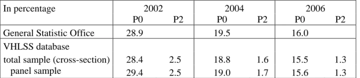
We focus on the panel subset of 1947 households who were followed through 2002-2004-2006.4 The panel dataset compares well in terms of poverty with national figures and with the entire VHLSS dataset (table A1
)
. According to the General Statistic Office, 28.9% of the population was below the poverty line in 2002. The figures for the same year are similar in the entire household survey (28.4%) and in the panel dataset (29.4%). The evolution of poverty is also similar.. Another hint of the good fit of the panel sample is given with respect to education (table A2). In 2002, 30.9% of the households’ heads in the entire survey had no education; they were 31% in the panel sample.Characterizing household economic activities
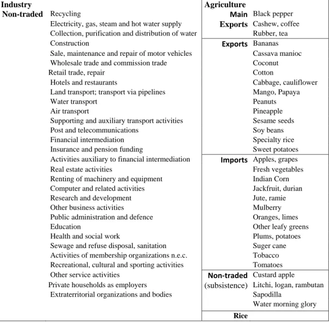
We start with the main sector of activity reported by each individual during the last twelve months. We then sum for each household the number of individuals who reported working in different sectors. For that purpose, the ISIC code of any sector was (manually) matched with the SITC classification used in trade data (COMTRADE and GSO statistics). A given sector is then classified as a net exporter or a net importer according to trade flows in 2002.
S
ectors that could not be matched with the trade data (mostly services) are classified as non-traded. The sector classification is given in table A3.Household members also report whether they are wage earners or self employed. The latter category is divided between self-employed working on farm and those working in non-farm activities. Unfortunately due to the questionnaire design, the answers are not exclusive. For instance, among 133 individuals who worked in aquaculture, 32 reported themselves as wage earners, 84 as self-employed and 17 declared themselves both wage earners and self employed.
3 The household questionnaire collects information on household composition, expenditures (disaggregated by
types), sources of income, employment and labor force participation, education (literacy, highest diploma, fee exemption), health of (use of health services, health insurance), housing (type of housing, electricity, water source, toilet), assets and durable goods and participation in poverty programs.
4
The panel linkage dataset was provided by Brian McCraig. The one provided by the statistical institute (GSO) showed some inconsistencies.
8
We thus define four categories: i) wage earners ii) self-employed on farm iii) self-employed in non-farm activities and iv) “multi-activity”. The latter includes all combinations of the former categories: being a wage earner and self-employed on farm; being a wage earner and self-employed in non-farm activities; being self-employed both on farm and out of the farm, etc. As a robustness check, we test an alternative grouping where categories are allowed to be non exclusive (section 7).As no data relate directly farmers’ production to external trade, we use the detailed list of crops grown on farm, as well as their share in total harvest and in total marketed output, and relate them to trade statistics (COMTRADE and GSO). Hence, crops are classified as export-oriented, import-competing or non-traded internationally (those are subsistence crops, often retained for own consumption). Among export crops, we further distinguish the main export crops which represent the bulk of Vietnam agricultural exports (such as tea, coffee, rubber, pepper and cashew).5 Rice, the main staple in Vietnam, is classified as a category on its own, as it is at the same time, exported, imported, locally consumed and retained for own consumption.
We are quite confident that households who grow main export crops are indeed mostly producing for international markets. Coello (2009) has shown that in 2002, cash crop producers sold on average more than 78% of their harvest, while households growing subsistence crops sold only 30% of their harvest, retaining the rest for own consumption. The corresponding share for rice producers is even lower, at 24% on average.
Consumer price index
Expenditures are deflated using an index that we have computed specifically. We start from regional and monthly indices of the cost of living, so as to take into account the spatial and time variation that occurred during the period the survey was conducted.6 The structure of expenditures and hence, the cost of living differ according to the position of a given household in the income distribution. Thus the shares of food and non-food consumption in the consumer price index differ by expenditures quintiles.
4. The method
Poverty
5 Harvests are valued in Vietnamese dongs, following Coello (2009) and Brandt, Benjamin and Coello (2009). 6 The regional and monthly consumer price indices were provided by Loren Brandt.
9
We use the concept of absolute poverty. Households are defined as poor if their real per capita expenditure is lower than the official poverty line.7 The Foster-Greer-Thorbecke (FGT) class of poverty indices writes:where N is the population size, z is the poverty line, the per capita expenditures of the i th household, I a dummy variable that takes the value of one if the condition is true and zero otherwise and α a poverty aversion parameter.
The headcount ratio represents the share of poor in total population. It is a particular case of the FGT index, where α is set to 0. Hence, it does not take into account the degree of poverty, and will not be affected by a policy that would further impoverish the poor. We also examine the severity of poverty, that is, the FGT index with α=2 (also named the squared poverty gap) that puts a greater weight on the poorest and is sensitive to the distribution below the poverty line. 8
We also look at poverty dynamics: a household can be either poor or not poor in 2002 and transit in or out poverty in 2004 and in 2006. The panel dataset provides a rare opportunity to compute these poverty transitions.
Econometric analysis
The econometric framework relates real per capita expenditures to households and local districts’ characteristics as well as trade-related contextual variables. We estimate a linear regression on panel data, in a reduced form, such as:
where is the level of real per capita expenditure of household i in year t, its change between 2002 and 2004, or 2004 and 2006. is a household fixed effect, are household variables that do not vary over time and control for initial endowments, is a vector of districts controls (that can be seen as the endowment in public goods). are the contextual variables that
7 In 2002 the official poverty line was set at 1,916,000 Dongs; in 2004, at 2,077 000 Dongs and in 2006 at 2,559
000 Dongs.
8 Another usual index is the poverty-gap (FGT with α=1), which represents the share of income needed in order
10
vary over time and relate to households’ sources of income (type of occupation, sector, and crops grown).Regressions are performed first on the whole population of the panel dataset, and next, specifically on farmers. 9 Contextual variables are first introduced per se (job types and sectors separately), then, as interacted variables (e.g. “wage earners working in export industries”).
The continuous approach, with the change in expenditures as the dependent variable, allows studying the impact of trade liberalization (here, taken as the change in the level of trade-related contextual variables). However, it assumes the same coefficients throughout the distribution. Thus, we also run the continuous regression on a sample restricted to households who were poor in 2002.
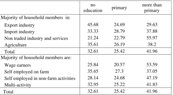
Table 2 details the variables and gives some descriptive statistics, with variables considered as the base category in the regression marked in parenthesis. Trade-related variables at the household level might of course be linked to other household characteristics. However, it is not in a linear and simple way. Table A4 shows households’ sector and job types by the level of education of the household head (as a proxy for each household member’s education). As could be expected, households with a majority of members earning wages are better educated (53.6% of household head have more than a primary education). However, households specialized in self-employed non-farm activities are not far below (47%). Regarding sectors, households with a majority of members in non-traded services are the most educated; households in import industries and agriculture share the same polarized pattern with respect to education of the head: they have either more than a primary education or on the contrary have not even completed primary education. Surprisingly, households specialized in export industries are the less skilled of all.
Robustness
We perform various robustness checks. First, we regress the change in expenditures to the
level of all variables in 2002, including the contextual ones. We have also mentioned in the previous
section, a second robustness check, which consists in changing the classification of job types and allowing them to be non exclusive (the “multi-activity” category disappears).10
A third robustness check uses a discrete regression, with poverty transitions as the dependent variable. This discrete form is usual in the literature and allows different coefficients depending on the
9
We also ran the same estimations on farmers controlling for the type of crops grown (such as cereals, fruits, annuals, perennials and vegetables). Results are similar and can be provided on request.
10
Regressions (not presented in the paper) were also performed without any contextual variables and generated similar results for the household and location characteristics.
11
poverty status. However, results may not be robust to a change in the level of the poverty line itself or to measurement errors that are frequent in household surveys (Glewwe 2005, Glewwe and Hoang Dang 2005). Moreover, crossing the poverty line changes the headcount, and hence, the type of transition, despite the fact that it could not mean much for the actual household (Ravallion 1996). That explains why our preferred specification is the continuous one.In the discrete approach, we use a multinomial logit regression on the probability of staying, exiting or entering into poverty. The multinomial logit model states that the probability that a household i is in state k is given by:
We examine the poverty transitions between 2002 and 2004 and between 2004 and 2006. The unordered choices (k) are (1) being poor in each period, (2) being non-poor in the first period and becoming poor in the second, (3) being poor in the first period and becoming non-poor in the second, and (4) being non-poor in both periods. Here again, we relate the multinomial logit to household and community characteristics as well as trade-related variables.
5. Household consumption and poverty in Vietnam, 2002-2006
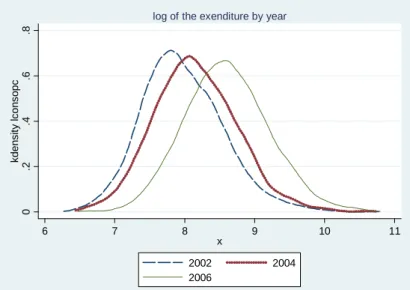
Figures 2 to 4 show the distribution of household expenditures per capita in Vietnam, in 2002, 2004 and 2006. The curves shifted to the right, especially between 2004 and 2006, the more so for food expenditures.
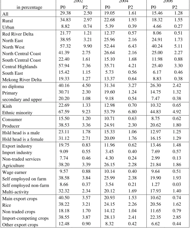
Table 3 displays the poverty indices computed on household expenditures in Vietnam. Between 2002 and 2006, the poverty incidence (P0) has been halved: 15.5% of the population are below the poverty line in 2006 compared to 30% in 2002 (first line). The corresponding headcounts in the 1990s were 58% in 1993 and 37% in 1998 (Glewwe et al. 2002). The drop in poverty in Vietnam over 20 years is indeed of a significant scale.
Most of the drop in poverty in the 2002-2006 period occurred between 2002 and 2004. The severity of poverty (P2) also drops by half in 2002-2006, down to 1.28% in 2006. In the 1990s, the severity of poverty was 7.9% in 1993 and dropped to 3.5% in 1998. Most of the drop in the 2002-2006 period occurred during the first two years.
12
The incidence of poverty is higher in rural areas (18.3% in 2006, second line) than in urban areas (4.7% in 2006).11 Poverty decreased in both types of areas, and more in 2002-2004.Vietnamese regions (figure A1) are historically very different: the South has been inhabited by Northern pioneers and was deeply influenced by the French and the American. Thus, regional differences mattered for economic growth in the 1990s (Brandt and Benjamin (2002); Coello (2008)). As regards poverty incidence, the poorest regions in 2002 were the North West (57% of the population were below the poverty line) and Central Highlands (57.9%) followed by North Central coast (41.4%) and North East (38.9%). In 2006, the North West has still a poverty incidence of 40.2%, but the other regions, and especially, the Central Highlands, have experienced a tremendous drop in poverty. This can be related to the specialization of Central Highlands in cash crop production (Benjamin et al. 2009, Coello 2009). The Central Coast in general and North Central Coast in particular is often affected by natural disasters, for instance, in 2005 by the Kai-Tak typhoon.12 As a result, the headcount decreased only slightly between 2004 and 2006 in North Central Coast and in the North East, and increased slightly in the South East. The severity of poverty even increased in 2004-2006 in the North Central Coast.
Poverty seems also related to low education, being in a household whose head is a woman and being from an ethnic minority. As regards activity, poverty is linked to being a farmer, growing main export crops (coffee, cashew, nuts, tea, pepper), as well as import-competing crops or rice. Again, poverty drops most among farmers growing export crops. It also dropped hugely for households in non-traded services, while it actually increased in 2004-2006 for households involved in import competing industries. These descriptive correlations seem to be in line with the expected effects of trade liberalization.
What is more unintuitive, is that the distribution among the poor matters. Poverty incidence decreased from 19 % in 2002 to 13% in 2006 for households working in export industries. However, the same households saw the severity of poverty increase in the meantime, from 0.6% in 2002 to 1.5% in 2006, particularly in 2004-2006. Households working in import industries also saw the severity of poverty slightly increase during this period.
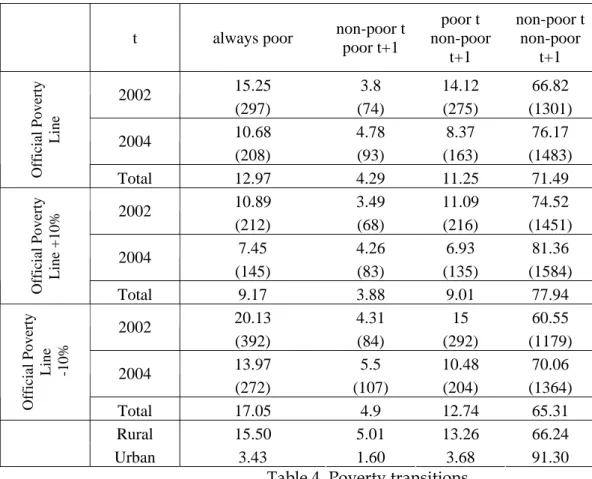
Table 4 shows the transitions in and out poverty during 2002-2006. Almost 13% of the population remains poor during the four years under study (third line). At the other extreme, “permanent” non-poor represent more than 71% of the panel households. The share of transitions out of poverty (11.2%) is more than double the share of transition into poverty (4.3%). In the 90s, for the
11
Comparable figures in 1993 are 66.4% in rural areas and 25.5% in urban areas (resp. 45.5% and 9.2% in 1998).
12
At least 19 people were killed and 10 others were left missing, the damages from the storm were estimated to be at least $11 million (2005 USD) (Source Emergency Events Database EM-DAT).
13
period 1993-98, Glewwe and al. (2002) found that 28.7% of the population was “permanent” poor; 39% were “permanent” non poor, 27.4% exited poverty and 4.8% entered into poverty. Hence, in the 2000s, most of the population has escaped poverty “permanently” at least in a four-year period. However, the share of “permanent” poor is not negligible, and the share of entry into poverty is quite constant in the 1990s and in the 2000s. And there is still a huge discrepancy between rural and urban areas (lines 10 and 11). 91% of urban households stay out of poverty during the period, while only 61% of rural households did so. 5% of rural households entered into poverty while it was the case for only 1.6% of urban households. 13The percentage of households going out of poverty decelerates in 2004-06 (8.4%) compared to 04 (14.1%). The share of poor households staying in poverty dropped also from 15.3% en 2002-04 to 10.7% in 202002-04-06.
As a sensitivity test, we set the poverty line 10% above and below the official level. With a poverty line higher by 10%, only 11.2% of households exit poverty in 2002-04 instead of 14.1%. The difference is smaller by 1.5% in 2004-2006. Alternatively, with a poverty line lower by 10%, the poverty exit rate is similar in 2002-04, and increase by two percentage points in 2004-06. These results indicate that between 2002 and 2004, individuals were just above the official poverty line: with a threshold 10% higher, the probability of exit drops significantly while when the threshold is lower by 10% nothing happens. In 2004-2006, on the opposite, households are equally distributed around the poverty line.
Figure 5 shows the kernel distribution of the relative distance of the per capita expenditure of the poor (in logarithm) to the poverty line. The relative distance to the poverty line is constructed exclusively on poor households. Within the poor, we measure the absolute difference between the households’ expenditure per capita and the official poverty line, divided by the official poverty line. The curve clearly shifts to the right in 2002-2006, meaning that the poor are moving farther below the poverty line. In other words, and in contradiction with the picture given by the headcount index alone, the poor in 2006 are less well off than the poor in 2002.
6. Trade liberalization and change in household expenditures
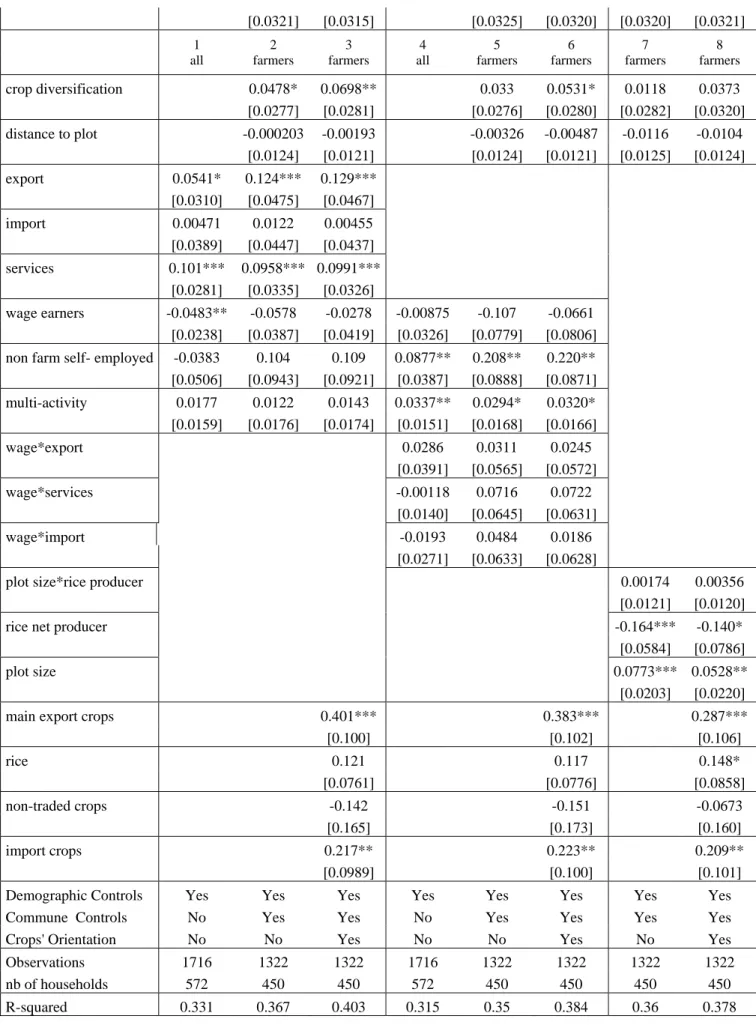
We now turn to the determinants of the expenditure growth in 2002-06 (table 5). The summary table below gives the main results.
13 The corresponding figures for rural areas in the same years (Justino and Lichfield 2003) were respectively,
14
variables that increase per capita household expenditure
variables that decrease per capita household expenditure
household share of adult female large household size
Characteristics share of adult male
being married number of children
household head is a woman being of an ethnic minority
household head has a primary education
household head has a secondary education
location living in a city
Characteristics living in South East living in the North Central region
living in Mekong River
village has access to electricity
farm
characteristics
share of land with a land-right certificate Trade-related
variables
1. job types nb of persons working in export industry
nb of persons working in import
competing industry
nb of persons working in services
2. sectors nb of wage earners a
nb of self-employed in non farm activities a
nb of multi-activity job holders
3. sectors*job
types wage earners in services b
wage earners in import competing industries b
4. farm being a rice net producer with a large plot
characteristics large plot size being a rice net producer
share of main export crops
share of subsistance crops
Notes: a positive when variables interacted with sector are added. b positive only for farmers.
With respect to household characteristics, the estimation results are in line with the descriptive statistics and with previous studies for the period 1993-98. The number of adults (male and female) has a positive impact on the increase in per capita expenditure between 2002 and 2006, contrary to the number of children. Being married is associated positively with income change, while belonging to an ethnic minority (non Kin) is negatively linked to income change. Other variables are less intuitive: having a woman as a household head, or having only completed primary education are associated positively with income changes. This positive effects could be related to the extent of overall growth in Vietnam which gave a chance to everybody. Location characteristics are also understandable: North Central region (hit by the typhoon) is associated with a negative income change, while the South (South East and the Mekong River) is associated with a positive income change. On the subsample of
15
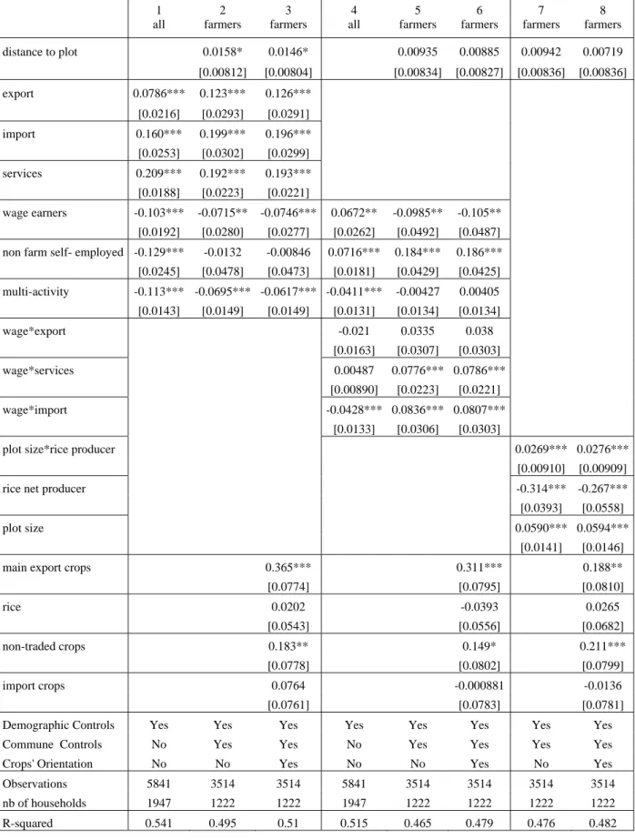
farmers, an increase in expenditure is associated with formal ownership (a larger share of land protected by a formal title of property) and with crops diversification.We now turn to the effect of the change in trade-related contextual variables. As expected, households with a larger number of persons working in export manufacturing industries, or farmers who have increased their specialization in export crops experience a rise in per capita expenditure. However, it is also the case for households involved in import-competing manufacture, or non-traded-services, as well as for farmers producing subsistence (non-traded) crops. Rice is a special case, as every farmer grows some rice. Thus, being a net producer of rice is associated negatively to income change. However, if the rice net producer owns a large plot, he is likely to experience a rise in income. Hence, trade openness has a distributional impact in the rice sector, differentiating between large and small producers. Overall, it seems that the benefit of the general growth of the economy exceeded the differential sectoral impact entailed by trade openness. In that context, it is interesting to note that households who increased their participation in multi-activity jobs experienced a decrease in their consumption growth. Thus, some specialization was needed to reap the benefits of overall growth, at least for the population as a whole.
When we restrict the analysis to households who were poor in 2002, the picture is somewhat different (table 6). The main results of the determinants of the consumption of the poor are presented in the summary table below, which also highlights the differences in the determinants of the consumption of the poor, compared to those of the general population.
Regarding household characteristics, gender seems to matter specifically on the consumption of poor households: having a larger share of adult female in the family is now clearly negatively correlated with expenditures; and having a woman as a household head has no longer a significant positive impact. Concerning the type of jobs, poor benefit indeed, as the total population, from export oriented industry and agriculture. However, for them, having some members earning wages is clearly linked to a decrease in income per capita (though the impact is still negative, but not significant anymore when variables interacting wage earnings and sector are added). In addition, poor farmers benefit not only from export crops, but also from import-competing crops (such as maize), which was not the case for the average household. Interestingly enough, even on the subsample of poor households, being a net producer of rice is still associated negatively to income. What matters for income change is the size of the plot. Finally, poor households benefit from being not specialized in one type of jobs and pursuing part-time multiple activities, contrary to the ordinary household in the total population.
variables that increase per capita
household expenditure of the poor
variables that decrease per capita household expenditure of the poor
16
share of adult male share of adult female *
(being married) number of children
(household head is a woman) being of an ethnic minority
household head has a primary
education
household head has a secondary
education
location characteristics (living in a city) **
living in South East living in the North Central region
living in Mekong River
village has access to electricity and
communication
farm characteristics share of land with a land-right certificate
nb of crops (crop diversification)
Trade related variables
1. job types nb of self-employed in non farm activities a *
nb of wage earners b
nb of multi-activity job holders a *
2. sectors nb of persons working in export industry
(nb of persons working in import
competing industry)
nb of persons working in services
3. sector*job types (wage earners in services) (wage earners in import competing industry)
4.farm characteristics (being a rice net producer with a large plot)
being a rice net producer
plot size
share of main export crops
(share of subsistance crops)
share of import competing crops *
Notes:
bold and * : sign changes when poor compared to total population.
italics and in parenthesis : not significant anymore in the subsample of the poor, compared to total population.
a
positive when variables interacted with sector are added.
b
: not significant when interacted variables are added
The picture that emerges from the econometric exercise is more complex than what a simple trade theory would predict. Indeed, exports both in industry and in agriculture matters. But poverty is not directly alleviated by the rise of a formal wages sector in for instance textile industry. As most of the poor are in rural areas and rely on agriculture, they benefit from market opportunities for the crops they produce as well as from new job opportunities in rural areas, such as transport or trading, in which they can involve on a part-time basis.
17
The first robustness check replicates the main regression, on all variables as of 2002 (table A5). Contextual variables are not anymore taken as changes between 2002 and 2006, but simply as their levels in 2002. Thus in this regression, we test how much the initial exposure to trade explains later performances. Actually, initial characteristics explain little of the subsequent change in expenditures: the R-squared drops from 54% in table 5 to 5%. Most contextual variables change sign even though they are not anymore significant. Working in the export industry in 2002 has a significant negative impact on subsequent consumption change. There are only two exceptions. First a specialization in main export crops still benefit farmers. Second, farmers involved in multi-activity jobs experience a decrease in their consumption growth. What can be inferred from this exercise is that the change in job opportunities in Vietnam during 2002 and 2006 in a broad sense (job types and sectors) was so significant that it has somewhat leveled the playing field. Initial positions in 2002 did not matter in determining subsequent income gains.A second robustness check consists in running the main estimation with an alternative definition of the types of jobs that allow for overlaps: an individual can be counted twice in two different categories (table A6). Results are similar to table 5 when no interacted variables are added. When the latter are added, the positive effect of self-employed non-farm activities attenuates. In parallel, wage jobs (but now, possibly mixed with self-employed profits) appear as having a strong positive impact, in any sector. Earning wages in import-competing industries and in services is positive for all households and not only for the sole farmers as in the main estimation. And wage jobs in export industry have now a positive impact for farmers. These results add to the point made above, of the complementing role of part-time activities.
The third robustness analysis examines the determinants of poverty transitions (table A7). In the multinomial logit, all results are given relative to the base category, which is a household who stays poor in both periods. Among the three poverty transitions, we will be particularly interested in the transition out of poverty of households who were initially poor. This transition compares quite well to the evolution of households who were poor in 2002, examined in table 6, even though they concern both the 2002-04 and the 2004-06 transitions. This notwithstanding, the main results of the transition out of poverty is presented in the summary table below.
variables that increase the probability of escaping poverty
variables that decrease the probability of escaping poverty household
characteristics share of adult male share of adult female
household head has a primary education share of children
household head has a secondary education
being of an ethnic minority
18
living in Mekong River
village has bus, train or water transport
farm characteristics crop diversification
Trade related variables
1. job types nb of wage earners
2. sectors nb of persons in services
3. sector*job types
nb of persons working as wage earners
in services
nb of persons working as wage earners in import competing industry
4.farm characteristics large plot
share of main export crops
share of rice
share of import competing crops
The determinants of the transition out of poverty fit quite well with the determinants of consumption growth of poor households. In both specifications, the share of adult male in the household, the education of household head (primary or secondary education) or living in the southern region (South East or Mekong river) are associated either with consumption growth or with a transition out of poverty. On the contrary, the share of adult female, the share of children, being of an ethnic minority, living in the North Central coast either impact negatively consumption growth or decrease the chance of escaping poverty.
The contextual variables give also similar results in both specifications. The number of wage earners in the family decrease the probability of escaping poverty, a paradoxical result already noted in the main estimation with poor’s consumption growth as the dependent variable. More precisely, wage earnings in services and import-competing industries raise the chances of getting out of poverty. Farmers owning a large plot, growing main export crops or rice or even import-competing crops have also a higher chance of escaping poverty. Hence, the significance of import-competing crops on poverty alleviation that was stressed in the consumption regression seems confirmed here. What is not confirmed in the multinomial logit is the role of self-employed non-farm activities and multi-activity jobs in the transition out of poverty. Coefficients have the right sign but are no longer significant. Actually, these variables matter significantly for households who stayed out of poverty all the time.
8. Conclusion
Vietnam trade liberalization occurred in two sub-periods. The first stage corresponded to the initial opening of the country in the nineties. It has been crucial for poverty alleviation and has been
19
extensively studied. However this first stage of trade opening concerned mostly exports, while domestic production and import-competing sectors were largely unaffected. In this paper, we explore the impact of the second stage of trade liberalization in the 2000s, as Vietnam deepens its openness to foreign competition, because of its involvement in a network of reciprocal trade agreements and its accession to the WTO.This paper shows the evolution of poverty in Vietnam during the deepening of trade liberalization and examines the impact of trade-related contextual variables, on occupational and crops choice, at the household level. Poverty decrease significantly during 2002 and 2006. However, this overall change hides a worsening of living conditions among the poor themselves especially in some regions (the North Central Coast) and some categories, among them, households involved in export and import industries.
In 2002-2006, Vietnamese households were impacted by external trade through different channels. First, as in the decade before, all activities (in industry as well as in agriculture) related to exports benefitted from trade openness. Moreover, unexpectedly, households involved in non-traded services and even in import-competing industry also gained.
Trade openness increased inequality among rice producers: it benefitted large producers, while it had a negative impact on small net producers. Farmers who intensified their specialization in the main exported crops (such as coffee, tea, cashew, pepper and rubber) obviously gained. But poor households also were better off if they were growing other crops such as maize, which was still protected at that time.
A robust and un-expected result is the negative effect of wage earnings per se on household consumption growth. The positive effect of trade openness on households did not occur through textbook channels such as the rise in (formal) unskilled wage jobs. Most households in Vietnam are still living in rural areas and working in agriculture. For them, poverty alleviation went through a rise in export crops production and a diversification of income sources, for instance, to non-farm self-employed (and often part-time) jobs. Wage earnings benefitted households not on all circumstances, but only depending on the sectors of employment. Last, besides exports, the import-competing sectors (in industry and in agriculture) played also a positive role in poverty alleviation. The latter channel could be hindered in the near future, as Vietnam is now in the process of decreasing its import protection.
20
TABLESin percentage 2002 2004 2006 total
Majority of household members are:
Wage earners 10.73 11.15 12.79 11.56
Self employed on farm 36.88 33.59 30.97 33.81
Self employed in non-farm activities 11.86 11.61 12.12 11.86
Multi-activity 40.52 43.66 44.12 42.77
Majority of household members in:
Export industry 4.16 4.73 2.67 3.85
Import industry 3.39 2.98 4.67 3.68
Non traded industry and services 23.22 26.3 29.17 26.23
Agriculture 69.23 66 63.48 66.24
Majority of agricultural production in:
Main export crops 6.21 6.63 5.8 6.21
Rice 48.38 47 49.46 48.28
Non-traded crops 8.47 8.73 5.29 7.5
Import-competing crops 8.53 9.86 9.19 9.19
Other export crops 28.4 27.79 30.25 28.81
Table 1. Employment and sector patterns Note : the column for each category sums to 100.
21
Name Definition Mean Std. Dev. Nb of obs
consumption growth Log of real per capita expenditure 8.242 0.652 5841
Red River Delta 0.191 0.393 5841
(North East) 0.146 0.354 5841
North West 0.042 0.201 5841
North Central Coast 0.125 0.331 5841
South Central Coast 0.099 0.298 5841
Central Highlands 0.065 0.246 5841
South East 0.117 0.321 5841
Mekong River Delta 0.215 0.411 5841
household size log hsld size 1.418 0.402 5841
age of household head log head age 3.825 0.293 5841
adult female Share female 18-60 0.282 0.162 5841
adult male Share male 18-60 0.269 0.169 5841
children Share children under 18 0.372 0.229 5841
ethnic minority =1, 0 otherwise 0.149 0.356 5841
married =1, 0 otherwise 0.828 0.377 5841
woman as head =1, 0 otherwise 0.218 0.413 5841
urban =1, 0 otherwise 0.210 0.407 5841
(No education) 0.326 0.469 5841
primary education primary education 0.254 0.435 5841
secondary education secondary and upper education 0.420 0.494 5841
daily market =1, 0 otherwise 0.415 0.493 4596
post office =1, 0 otherwise 0.419 0.493 4596
transport Bus, train water transport (=1, 0 otherwise) 0.396 0.489 4596
electricity =1, 0 otherwise 0.943 0.232 5745
land rights Share of land with certificate in 2004 0.713 0.406 5607
crop diversification log of number of crops 1.482 0.826 4162
distance to plot distance to the agricultural plot 6.308 1.374 4146
(share of other export in harvest value) 0.142 0.218 4162
main export crops harvest share of main export crops 0.076 0.232 4162
rice harvest share of rice 0.545 0.369 4162
subsistence crops harvest share of subsistence crops 0.115 0.207 4162
import crops harvest share of import competing crops 0.121 0.211 4162
(agriculture) (nbr pers in agriculture) 1.501 1.441 5841
export nbr pers in export industry 0.180 0.549 5841
import nbr pers in import-competing industry 0.171 0.522 5841
services nbr pers in non-traded services 0.740 0.981 5841
(nbr pers only self-employed on farm) 1.069 1.275 5841
wage earners nbr of wages earners 0.451 0.845 5841
non farm self- employed nbr pers of non-farm self-employed 0.270 0.649 5841
multi-activity nb of pers earning wages and self-employed 0.804 0.964 5841
plot size*rice total area*producer of rice 10645 18391 4085
rice net producer =1 if hsld is net producer of rice, 0 otherwise 0.585 0.493 5841
22
Table 2 : Variables definition and statistics
2002 2004 2006
in percentage P0 P2 P0 P2 P0 P2
All 29.38 2.50 19.05 1.61 15.46 1.28
Rural 34.83 2.97 22.68 1.93 18.32 1.55
Urban 8.82 0.74 5.39 0.39 4.66 0.27
Red River Delta 21.77 1.21 12.37 0.57 8.06 0.51
North East 38.95 3.21 25.96 2.16 24.91 1.73
North West 57.32 9.90 52.44 6.43 40.24 5.11
North Central Coast 41.39 2.75 26.64 2.16 25.00 2.27
South Central Coast 22.40 1.61 15.10 1.68 11.98 0.88
Central Highlands 57.94 7.36 35.71 4.21 25.40 3.30
South East 15.42 1.15 5.73 0.56 6.17 0.46
Mekong River Delta 19.33 1.27 13.37 0.64 8.83 0.38
no diploma 40.16 4.50 31.34 3.27 26.30 2.42
Primary 30.71 2.30 19.60 1.24 14.75 1.32
secondary and upper 20.20 1.08 9.18 0.54 7.47 0.38
Kinh 22.69 1.33 12.98 0.70 10.32 0.65 Ethnic minority 67.59 9.23 53.79 6.80 44.83 4.92 Consumer 15.50 1.20 10.71 0.63 8.75 0.62 Producer 38.53 3.36 24.91 2.30 20.62 1.80 Hsld head is a male 23.11 1.78 15.33 1.06 12.97 1.25 Hsld head is a female 31.12 2.71 20.09 1.76 16.15 1.29 Export industry 19.75 0.83 11.96 0.62 13.46 1.48 Import industry 9.09 0.55 3.45 0.40 7.69 0.57 Non-traded services 7.74 0.46 4.30 0.24 2.99 0.13 Agriculture 38.20 3.39 26.15 2.28 21.84 1.86 Wage earner 9.57 0.88 10.14 0.40 9.64 0.51
Self employed on farm 38.58 3.84 25.99 2.38 19.90 1.93
Self employed non-farm 8.66 0.37 3.54 0.21 1.27 0.03
Multi-activity 32.32 2.34 20.12 1.69 17.93 1.40
Main export crops 40.50 3.57 20.93 1.53 10.62 0.74
Rice 38.22 3.21 24.15 2.26 20.56 1.62
Non traded crops 18.18 1.70 14.12 1.04 11.65 0.79
Import-competing crops 38.55 3.87 28.13 2.41 22.35 2.85
Other export crops 12.48 0.90 8.32 0.42 6.62 0.44
Table 3. Poverty indices by socioeconomic characteristics Note : P0 headcount P2 severity of poverty
23
t always poor non-poor t
poor t+1 poor t non-poor t+1 non-poor t non-poor t+1 15.25 3.8 14.12 66.82 2002 (297) (74) (275) (1301) 10.68 4.78 8.37 76.17 2004 (208) (93) (163) (1483) Official Povert y Line Total 12.97 4.29 11.25 71.49 10.89 3.49 11.09 74.52 2002 (212) (68) (216) (1451) 7.45 4.26 6.93 81.36 2004 (145) (83) (135) (1584) Official Povert y Li ne + 10% Total 9.17 3.88 9.01 77.94 20.13 4.31 15 60.55 2002 (392) (84) (292) (1179) 13.97 5.5 10.48 70.06 2004 (272) (107) (204) (1364) Official Povert y Line -10% Total 17.05 4.9 12.74 65.31 Rural 15.50 5.01 13.26 66.24 Urban 3.43 1.60 3.68 91.30
Table 4. Poverty transitions
Note: The year reported on the second column is the initial year of the transition. Thus row one shows the transition from year 2002 to year 2004 and row two from year 2004 to year2006. A row sums up to 100. Number of households in each category is in parenthesis.
25
1 2 3 4 5 6 7 8
all farmers farmers all farmers farmers farmers farmers
Red River Delta -0.00854 -0.0292 0.00429 0.0108 -0.00727 0.026 0.00845 0.0234
[0.0322] [0.0364] [0.0365] [0.0330] [0.0374] [0.0374] [0.0369] [0.0372]
North West -0.0786 -0.016 -0.0251 -0.0642 0.00213 -0.00688 -0.0378 -0.0297
[0.0479] [0.0530] [0.0530] [0.0492] [0.0546] [0.0546] [0.0541] [0.0546]
North Central Coast -0.139*** -0.124*** -0.0892** -0.135*** -0.132*** -0.100** -0.141*** -0.119***
[0.0343] [0.0387] [0.0388] [0.0353] [0.0399] [0.0400] [0.0393] [0.0398]
South Central Coast 0.0407 0.00909 0.0375 0.0698* 0.0425 0.066 0.0211 0.041
[0.0376] [0.0459] [0.0460] [0.0385] [0.0472] [0.0473] [0.0465] [0.0471]
Central Highlands 0.0566 0.137*** 0.0213 0.0149 0.0820* -0.0364 -0.0769 -0.105*
[0.0413] [0.0478] [0.0536] [0.0422] [0.0489] [0.0549] [0.0512] [0.0558]
South East 0.315*** 0.380*** 0.307*** 0.297*** 0.333*** 0.254*** 0.183*** 0.161***
[0.0360] [0.0519] [0.0540] [0.0371] [0.0532] [0.0553] [0.0550] [0.0573]
Mekong River Delta 0.220*** 0.380*** 0.403*** 0.200*** 0.332*** 0.352*** 0.185*** 0.198***
[0.0325] [0.0464] [0.0461] [0.0335] [0.0474] [0.0472] [0.0497] [0.0502]
household size -0.186*** -0.237*** -0.243*** -0.171*** -0.202*** -0.206*** -0.180*** -0.182***
[0.0323] [0.0399] [0.0396] [0.0331] [0.0409] [0.0406] [0.0387] [0.0386]
age of the head 0.241*** 0.223*** 0.233*** 0.235*** 0.231*** 0.241*** 0.219*** 0.220***
[0.0419] [0.0468] [0.0463] [0.0431] [0.0482] [0.0477] [0.0475] [0.0474] female adults 0.114** 0.113 0.114 0.127** 0.147** 0.153** 0.122* 0.120* [0.0577] [0.0704] [0.0697] [0.0594] [0.0725] [0.0718] [0.0716] [0.0714] male adults 0.329*** 0.358*** 0.372*** 0.353*** 0.385*** 0.398*** 0.354*** 0.362*** [0.0602] [0.0710] [0.0702] [0.0618] [0.0732] [0.0724] [0.0713] [0.0712] children -0.223*** -0.157** -0.138* -0.255*** -0.186** -0.167** -0.261*** -0.261*** [0.0650] [0.0738] [0.0730] [0.0668] [0.0759] [0.0751] [0.0754] [0.0752] ethnic minority -0.224*** -0.222*** -0.194*** -0.274*** -0.251*** -0.223*** -0.270*** -0.253*** [0.0300] [0.0332] [0.0332] [0.0305] [0.0341] [0.0340] [0.0337] [0.0339] married 0.116*** 0.0916** 0.0940** 0.125*** 0.0855* 0.0861** 0.0843* 0.0843* [0.0329] [0.0426] [0.0422] [0.0339] [0.0439] [0.0435] [0.0433] [0.0432] woman as head 0.0832*** 0.0254 0.034 0.0895*** 0.0244 0.0315 0.0377 0.0432 [0.0283] [0.0397] [0.0392] [0.0291] [0.0409] [0.0404] [0.0402] [0.0401] urban 0.300*** 0.320*** [0.0245] [0.0252] primary education 0.142*** 0.141*** 0.145*** 0.158*** 0.156*** 0.162*** 0.156*** 0.161*** [0.0240] [0.0271] [0.0268] [0.0246] [0.0278] [0.0276] [0.0274] [0.0274] secondary education 0.363*** 0.303*** 0.300*** 0.391*** 0.333*** 0.332*** 0.329*** 0.327*** [0.0245] [0.0282] [0.0279] [0.0250] [0.0287] [0.0285] [0.0283] [0.0283] daily market 0.000601 -0.0008 -0.000198 0.000678 0.00175 0.000409 [0.0242] [0.0240] [0.0249] [0.0247] [0.0246] [0.0245] post office -0.0112 -0.00271 -0.0113 -0.00433 -0.00938 -0.00438 [0.0231] [0.0229] [0.0238] [0.0236] [0.0235] [0.0235] transport 0.015 0.0156 0.0296 0.0298 0.0119 0.0112 [0.0225] [0.0222] [0.0232] [0.0229] [0.0228] [0.0227] electricity 0.129*** 0.105** 0.143*** 0.117*** 0.145*** 0.126*** [0.0429] [0.0427] [0.0442] [0.0439] [0.0436] [0.0438] land rights 0.106*** 0.110*** 0.110*** 0.116*** 0.124*** 0.122*** [0.0273] [0.0270] [0.0280] [0.0278] [0.0277] [0.0277] crop diversification 0.0672*** 0.0632*** 0.0386** 0.0312 0.00983 0.00414 [0.0190] [0.0193] [0.0193] [0.0196] [0.0191] [0.0216]
26
1 2 3 4 5 6 7 8
all farmers farmers all farmers farmers farmers farmers
distance to plot 0.0158* 0.0146* 0.00935 0.00885 0.00942 0.00719 [0.00812] [0.00804] [0.00834] [0.00827] [0.00836] [0.00836] export 0.0786*** 0.123*** 0.126*** [0.0216] [0.0293] [0.0291] import 0.160*** 0.199*** 0.196*** [0.0253] [0.0302] [0.0299] services 0.209*** 0.192*** 0.193*** [0.0188] [0.0223] [0.0221] wage earners -0.103*** -0.0715** -0.0746*** 0.0672** -0.0985** -0.105** [0.0192] [0.0280] [0.0277] [0.0262] [0.0492] [0.0487]
non farm self- employed -0.129*** -0.0132 -0.00846 0.0716*** 0.184*** 0.186***
[0.0245] [0.0478] [0.0473] [0.0181] [0.0429] [0.0425] multi-activity -0.113*** -0.0695*** -0.0617*** -0.0411*** -0.00427 0.00405 [0.0143] [0.0149] [0.0149] [0.0131] [0.0134] [0.0134] wage*export -0.021 0.0335 0.038 [0.0163] [0.0307] [0.0303] wage*services 0.00487 0.0776*** 0.0786*** [0.00890] [0.0223] [0.0221] wage*import -0.0428*** 0.0836*** 0.0807*** [0.0133] [0.0306] [0.0303]
plot size*rice producer 0.0269*** 0.0276***
[0.00910] [0.00909]
rice net producer -0.314*** -0.267***
[0.0393] [0.0558]
plot size 0.0590*** 0.0594***
[0.0141] [0.0146]
main export crops 0.365*** 0.311*** 0.188**
[0.0774] [0.0795] [0.0810] rice 0.0202 -0.0393 0.0265 [0.0543] [0.0556] [0.0682] non-traded crops 0.183** 0.149* 0.211*** [0.0778] [0.0802] [0.0799] import crops 0.0764 -0.000881 -0.0136 [0.0761] [0.0783] [0.0781]
Demographic Controls Yes Yes Yes Yes Yes Yes Yes Yes
Commune Controls No Yes Yes No Yes Yes Yes Yes
Crops' Orientation No No Yes No No Yes No Yes
Observations 5841 3514 3514 5841 3514 3514 3514 3514
nb of households 1947 1222 1222 1947 1222 1222 1222 1222
R-squared 0.541 0.495 0.51 0.515 0.465 0.479 0.476 0.482
Table 5. Determinants of consumption growth (2002-2006)
Note : dependent variable : real per capita expenditures. A * (resp ** and ****) show significance at 90% (95%, 99%) of confidence. Standard errors in brackets.
27
1 2 3 4 5 6 7 8
all farmers farmers all farmers farmers farmers farmers
Red River Delta -0.0643 -0.0573 -0.0187 -0.0548 -0.0375 -0.000972 -0.036 -0.0097 [0.0426] [0.0484] [0.0484] [0.0431] [0.0488] [0.0491] [0.0480] [0.0489] North West -0.0619 -0.0283 -0.0378 -0.0582 -0.0184 -0.029 -0.0393 -0.0396 [0.0455] [0.0520] [0.0514] [0.0460] [0.0524] [0.0519] [0.0516] [0.0523] North Central Coast -0.117*** -0.110** -0.0707 -0.121*** -0.106** -0.069 -0.121*** -0.0895* [0.0389] [0.0450] [0.0454] [0.0393] [0.0456] [0.0462] [0.0448] [0.0460] South Central Coast -0.0442 -0.0272 0.0199 -0.0247 -0.0147 0.0306 -0.0124 0.0324 [0.0511] [0.0591] [0.0591] [0.0514] [0.0600] [0.0601] [0.0591] [0.0604] Central Highlands 0.00368 0.0412 -0.0322 -0.0162 0.024 -0.0468 -0.0422 -0.0552 [0.0412] [0.0510] [0.0555] [0.0416] [0.0512] [0.0560] [0.0527] [0.0562] South East 0.101* 0.190** 0.123 0.0839 0.160** 0.098 0.105 0.102 [0.0533] [0.0772] [0.0793] [0.0540] [0.0788] [0.0814] [0.0784] [0.0822] Mekong River Delta 0.100** 0.149** 0.179*** 0.0761* 0.132* 0.156** 0.0667 0.106 [0.0452] [0.0688] [0.0687] [0.0461] [0.0686] [0.0689] [0.0686] [0.0702] household size -0.0518 -0.0919* -0.0946* -0.0389 -0.0704 -0.0714 -0.0905* -0.0778 [0.0454] [0.0535] [0.0523] [0.0459] [0.0539] [0.0528] [0.0532] [0.0533] age of the head 0.0597 0.00522 -0.0118 0.0513 0.00618 -0.00892 0.013 0.00274 [0.0464] [0.0522] [0.0515] [0.0468] [0.0527] [0.0522] [0.0521] [0.0519] female adults -0.173** -0.141 -0.137 -0.178** -0.145 -0.143 -0.147 -0.141 [0.0875] [0.107] [0.105] [0.0885] [0.109] [0.107] [0.108] [0.107] male adults 0.109 0.252** 0.226** 0.117 0.268** 0.241** 0.245** 0.247** [0.0949] [0.108] [0.106] [0.0961] [0.110] [0.108] [0.107] [0.107] children -0.134* -0.0291 -0.0341 -0.133 -0.0328 -0.0393 -0.0711 -0.0544 [0.0806] [0.0927] [0.0905] [0.0818] [0.0939] [0.0920] [0.0932] [0.0929] ethnic minority -0.194*** -0.202*** -0.183*** -0.217*** -0.213*** -0.195*** -0.227*** -0.216*** [0.0310] [0.0361] [0.0358] [0.0309] [0.0363] [0.0361] [0.0359] [0.0362] married 0.0192 -0.0237 -0.0268 0.0229 -0.0197 -0.0219 -0.0146 -0.0197 [0.0493] [0.0571] [0.0557] [0.0496] [0.0571] [0.0559] [0.0566] [0.0561] woman as head 0.0392 -0.00598 0.00233 0.0459 -0.0024 0.00664 0.00918 0.0103 [0.0468] [0.0555] [0.0542] [0.0472] [0.0560] [0.0548] [0.0553] [0.0549] urban 0.0591 0 0 0.067 0 0 0 0 [0.0462] [0] [0] [0.0470] [0] [0] [0] [0] primary education 0.0924*** 0.0852** 0.0804** 0.0985*** 0.0906*** 0.0866*** 0.110*** 0.101*** [0.0281] [0.0331] [0.0324] [0.0283] [0.0334] [0.0328] [0.0330] [0.0328] secondary education 0.204*** 0.180*** 0.162*** 0.212*** 0.193*** 0.177*** 0.202*** 0.186*** [0.0304] [0.0345] [0.0341] [0.0307] [0.0347] [0.0345] [0.0343] [0.0345] daily market -0.0086 -0.0198 -0.000556 -0.011 0.0105 -0.00166 [0.0312] [0.0306] [0.0314] [0.0308] [0.0310] [0.0309] post office -0.0483 -0.0403 -0.0446 -0.0362 -0.0531* -0.0498* [0.0296] [0.0290] [0.0301] [0.0296] [0.0295] [0.0295] transport 0.0289 0.0369 0.0349 0.0435 0.0394 0.0464 [0.0290] [0.0285] [0.0293] [0.0288] [0.0283] [0.0282] electricity 0.0992** 0.0973** 0.104** 0.103** 0.114*** 0.112*** [0.0403] [0.0396] [0.0407] [0.0402] [0.0401] [0.0402] land rights 0.0819** 0.0886*** 0.0855*** 0.0905*** 0.0938*** 0.0961***
28
[0.0321] [0.0315] [0.0325] [0.0320] [0.0320] [0.0321]1 2 3 4 5 6 7 8
all farmers farmers all farmers farmers farmers farmers
crop diversification 0.0478* 0.0698** 0.033 0.0531* 0.0118 0.0373 [0.0277] [0.0281] [0.0276] [0.0280] [0.0282] [0.0320] distance to plot -0.000203 -0.00193 -0.00326 -0.00487 -0.0116 -0.0104 [0.0124] [0.0121] [0.0124] [0.0121] [0.0125] [0.0124] export 0.0541* 0.124*** 0.129*** [0.0310] [0.0475] [0.0467] import 0.00471 0.0122 0.00455 [0.0389] [0.0447] [0.0437] services 0.101*** 0.0958*** 0.0991*** [0.0281] [0.0335] [0.0326] wage earners -0.0483** -0.0578 -0.0278 -0.00875 -0.107 -0.0661 [0.0238] [0.0387] [0.0419] [0.0326] [0.0779] [0.0806] non farm self- employed -0.0383 0.104 0.109 0.0877** 0.208** 0.220** [0.0506] [0.0943] [0.0921] [0.0387] [0.0888] [0.0871] multi-activity 0.0177 0.0122 0.0143 0.0337** 0.0294* 0.0320* [0.0159] [0.0176] [0.0174] [0.0151] [0.0168] [0.0166] wage*export 0.0286 0.0311 0.0245 [0.0391] [0.0565] [0.0572] wage*services -0.00118 0.0716 0.0722 [0.0140] [0.0645] [0.0631] wage*import -0.0193 0.0484 0.0186 [0.0271] [0.0633] [0.0628]
plot size*rice producer 0.00174 0.00356
[0.0121] [0.0120]
rice net producer -0.164*** -0.140*
[0.0584] [0.0786]
plot size 0.0773*** 0.0528**
[0.0203] [0.0220]
main export crops 0.401*** 0.383*** 0.287***
[0.100] [0.102] [0.106] rice 0.121 0.117 0.148* [0.0761] [0.0776] [0.0858] non-traded crops -0.142 -0.151 -0.0673 [0.165] [0.173] [0.160] import crops 0.217** 0.223** 0.209** [0.0989] [0.100] [0.101]
Demographic Controls Yes Yes Yes Yes Yes Yes Yes Yes
Commune Controls No Yes Yes No Yes Yes Yes Yes
Crops' Orientation No No Yes No No Yes No Yes
Observations 1716 1322 1322 1716 1322 1322 1322 1322
nb of households 572 450 450 572 450 450 450 450
R-squared 0.331 0.367 0.403 0.315 0.35 0.384 0.36 0.378
Table 6 : Determinants of consumption growth for initially poor households Note : dependent variable : real per capita expenditures. Sample restricted to poor households in 2002. A * (resp ** and ****) show significance at 90% (95%, 99%) of confidence. Standard errors in brackets.
30
FIGURES
Figure 1. Weighted tariffs by type of products (Source TRAINS)
0 .2 .4 .6 .8 kd e n si ty l c o n so p c 6 7 8 9 10 11 x 2002 2004 2006
log of the exenditure by year
Figure 2. Kernel density function of the expenditure per capita by year
0 .2 .4 .6 .8 kd e n sity l c on s o fd p c p x 0 4 6 7 8 9 10 11 x 2002 2004 2006
log of the food exenditure pc by year
Figure 3. Kernel density function of the food consumption
per capita by year
0 .2 .4 .6 .8 kd e n si ty l c on s o n o fp c p x0 4 4 6 8 10 12 x 2002 2004 2006
log of the no-food exenditure pc by year
Figure 4.
Kernel density function
of the non food consumption per
31
0 .1 .2 .3 .4 k d e n s it y ld is tr el -10 -5 0 5 x 2002 2004 2006log of the relative distance to the poverty line by year
Figure 5. Kernel density function of the relative distance in log to the poverty line by
year
32
REFERENCES
Athukorala P-C, 2006. Trade Policy Reforms and the structure of protection in Vietnam. Departmental Working Papers 2005-06, Australian National University, Economics RSPAS.
Auffret P.2003. Trade Reform in Vietnam Opportunities with Emerging Challenges. World Bank
Policy Research Working Paper No. 3076.
Benjamin D. & Brandt L.2002. Agriculture and Income Distribution in Rural Vietnam under
Economic Reforms: A Tale of Two Regions. William Davidson Institute Working Papers Series 519. Coello B., 2008. Agriculture and trade liberalization in Vietnam. Working Paper 75, Paris School of Economics.
Coello B. 2009. Impact of exports liberalization and specialization in cash crop what are the expected gains for Vietnamese households” Economie Internationale,118 (2), pp.73-99
Benjamin D., Brandt L. and Coello B.2009 “Vietnam crop output report 1993-2006”
Dercon S. Shapiro J. 2007. Moving On, Staying Behind, Getting Lost: Lessons on poverty mobility from longitudinal data, in D.Narayan and P.Petesch, Moving out of Poverty, Palgrave McMillan and World Bank.
Dollar, D., Kraay, A., 2004 Trade, Growth, and Poverty. Economic Journal, Vol. 114, pp. F22-F49. Edmonds E. and Pavcnik, N.2004. Product Market Integration and Household Labor Supply in a Poor Economy: Evidence from Vietnam, World Bank Policy Research Working Paper #3234.
Edwards, Sebastian, 1998."Openness, Productivity and Growth: What Do We Really Know?," Economic Journal, Royal Economic Society, vol. 108(447), pages 383-98, March.
Gallup J. L. 2003. The Wage Labor Market and Inequality in Vietnam in the 1990s World Bank Policy Research Working Paper No. 2896.
General Statistic Office of Vietnam, http://www.gso.gov.vn/default_en.aspx?tabid=491
Glewwe, P. 2005. How much of observed economic mobility is measurement error ? a method to reduce measurement error bias, with an application to Vietnam, mimeo.
Glewwe, P., Hoang Dang, H-A., 2005. Was Vietnam’s Economic growth in the 1990’s pro-poor ? an analysis of panel data from Vietnam, mimeo
Glewwe, P.; Gragnolati, M.; Zaman, H.2002 Who gained from Vietnam’s boom in the 1990’s. in: Economic Development and Cultural Change, v.50, no.4, July, pp.773-792, 2002.
Glewwe, P., Vu L. 2008. Impact of rising food prices on poverty and welfare in Vietnam. Working paper , Department of Applied economics, University of Minnesota.