HAL Id: hal-00414395
https://hal.archives-ouvertes.fr/hal-00414395
Submitted on 9 Sep 2009
HAL is a multi-disciplinary open access archive for the deposit and dissemination of sci-entific research documents, whether they are pub-lished or not. The documents may come from teaching and research institutions in France or abroad, or from public or private research centers.
L’archive ouverte pluridisciplinaire HAL, est destinée au dépôt et à la diffusion de documents scientifiques de niveau recherche, publiés ou non, émanant des établissements d’enseignement et de recherche français ou étrangers, des laboratoires publics ou privés.
Real time plasma equilibrium reconstruction in a
Tokamak
Jacques Blum, Cédric Boulbe, Blaise Faugeras
To cite this version:
Jacques Blum, Cédric Boulbe, Blaise Faugeras. Real time plasma equilibrium reconstruction in a Tokamak. ICIPE 2008: 6th Int. Conf. on Inverse Problems in Engineering, Jun 2008, Dourdan, France. p 12-19, �10.1088/1742-6596/135/1/012019�. �hal-00414395�
Real-time plasma equilibrium reconstruction in a
Tokamak.
J. Blum, C. Boulbe and B. Faugeras
Laboratoire J.A. Dieudonn´e, UMR 6621, Universit´e de Nice Sophia Antipolis, Parc Valrose, 06108 Nice Cedex 02, France
E-mail: [email protected], [email protected], [email protected]
Abstract. The problem of equilibrium of a plasma in a Tokamak is a free boundary problem described by the Grad-Shafranov equation in axisymmetric configurations. The right hand side of this equation is a non linear source, which represents the toroidal component of the plasma current density. This paper deals with the real time identification of this non linear source from experimental measurements. The proposed method is based on a fixed point algorithm, a finite element resolution, a reduced basis method and a least-square optimization formulation.
1. Introduction
In Tokamaks, a magnetic field is used to confine a plasma in a toroidal vacuum vessel. The magnetic field is produced by external coils surrounding the vacuum vessel and a current circulating in the plasma, forming a helicoidal resulting magnetic field. At equilibrium, magnetic field lines lie on isosurfaces forming a family of nested tori and called magnetic surfaces. These magnetic surfaces enable to define the magnetic axis and the plasma boundary. The innermost magnetic surface which degenerates into a closed curve is called magnetic axis. The plasma boundary corresponds to the surface in contact with a limiter or being a magnetic separatrix (hyperbolic line with an X-point).
Denote by j the current density, B the magnetic field and p the kinetic pressure. The equilibrium of the plasma in presence of a magnetic field is described by
j = ∇ ×B
µ, (1)
j× B = ∇p, (2)
∇ · B = 0, (3)
where µ is the magnetic permeability. Equation (1) is Ampere’s theorem and equation (3) represents the conservation of magnetic induction. Equation (2) means that at equilibrium the Lorentz force j × B balances the force ∇p due to kinetic pressure. From this equation it is clear that
B· ∇p = 0 and j · ∇p = 0. (4)
Thus, p is constant along magnetic field lines and current lines which consequently lie on magnetic surfaces.
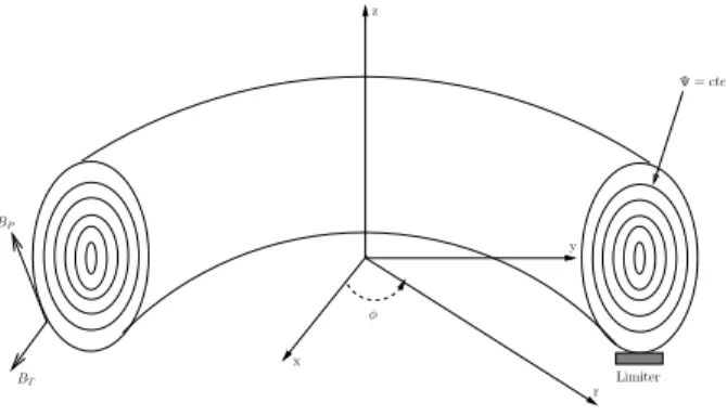
x r y z BT Limiter Ψ = cte φ BP
Figure 1. Toroidal geometry.
Consider the cylindrical coordinate system (r, z, φ). Under axisymmetrical hypothesis, the magnetic field is supposed to be independent of the toroidal angle φ and can be decomposed in the form B= BP + BT BP = 1 r[∇ψ × eφ] BT = f reφ (5)
where BP and BT are respectively the poloidal and the toroidal component of the magnetic
field, eφ is a unit vector in direction φ,the term ψ(r, z) is the poloidal magnetic flux function
(see Figure 1) and f is the poloidal current flux function. The magnetic surfaces are defined by rotation of the flux lines ψ = constant around the vertical axis (Oz). Using (5), equations (1)-(3) lead to the Grad-Shafranov equation (see [1, 2, 3])
− ∆∗ψ= rp′(ψ) + 1 µ0r (f f′)(ψ) (6) where ∆∗.= ∂ ∂r( 1 µ0r ∂. ∂r) + ∂ ∂z( 1 µ0r ∂. ∂z). (7)
and µ0 is the magnetic permeability of the vacuum. Thus, under axisymmetric hypothesis, the
three dimensional equilibrium (1)-(3) reduces to solve a two dimensional non-linear problem. Note that the right hand side of (6) represents the toroidal component jφ of the plasma current
density which is determinated by p′, f and f′.
In this paper, we are interested in the numerical reconstruction of the plasma current density and of the equilibrium (6) (see [4, 5, 6]). This reconstruction has to be achieved in real time from experimental measurements. The main difficulty consists in identifying the functions p′ and f f′ in the non linear source term of (6). An iterative strategy involving a finite element method to solve the direct problem (6) and a least square optimisation procedure to identify the non linearity using reduced basis is proposed. A description of the experimental measurements available in Tokamaks is given in Section 2. Section 3 is devoted to the statement of the mathematical problem and the numerical algorithm proposed. Numerical results obtained with the software Equinox are presented in Section 4.
2. Experimental measurements
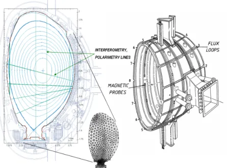
Although p and f cannot be directly measured in a Tokamak, several measurements are available (see Figure 2):
• magnetic measurements: the flux loops provide Dirichlet condition ψ = h and magnetic probes Neumann condition 1
r ∂ψ
∂n = g on the walls of the vacuum vessel which represent the boundary of the computational domain. These measurements are given at some discrete points Ni and the Dirichlet full boundary data are obtained by interpolation.
• polarimetric measurements: this measurement gives the value of the integral along a family of chords Ci Z Ci ne r ∂ψ ∂ndl= αi.
ne(ψ) is the electronic density which is approximately constant on each flux line, ∂ψ ∂n is the normal derivative of ψ along the chord Ci.
• interferometric measurements: they give the values of the integrals
Z
Ci
nedl= βi.
• current measurements: they give the value of the total plasma current Ip defined by
Ip =
Z
Ωp
jφdx.
Other measurements are potentially available but are not used for the moment in the software Equinox.
Figure 2. Left: the straight green lines represent the chords used for polarimetry and interferometry measurements. Right: part of the vacuum vessel including the magnetic measurements. At the bottom middle an example of finite element mesh used for numerical simulations.
3. Algorithm and numerical resolution
Let Ω be the domain representing the vacuum vessel of the Tokamak, and ∂Ω its boundary. The equilibrium of a plasma in a Tokamak is a free boundary problem. The plasma boundary is
determinated either by its contact with a limiter D or as being a magnetic separatrix with an X-point (hyperbolic point). The region Ωp ⊂ Ω containing the plasma is defined by
Ωp= {x ∈ Ω, ψ(x) ≥ ψb}
where ψb = maxDψ in the limiter configuration or ψb = ψ(X) when an X-point exists.
In the vacuum region, the right hand side of (6) vanishes and the equilibrium reads ∆∗ψ= 0 in Ω \ Ωp
Consider the following notations: ψ¯ =
ψ− max Ω ψ ψb− max Ω ψ ∈ [0, 1] in Ωp , A( ¯ψ) = R0 λ p ′(ψ) and B( ¯ψ) = 1 λµ0R0
(f f′)(ψ). The functions A and B are flux functions defined on the fixed interval [0, 1]. Giving Dirichlet boundary conditions, the final equilibrium problem is
−∆∗ψ = λ[ r R0 A( ¯ψ) +R0 r B( ¯ψ)]χΩp in Ω ψ = h on ∂Ω (8)
where χΩp is the characteristic function of Ωp and R0 is the major radius of the Tokamak. The
parameter λ is a normalization factor that satisfies Ip = λ Z Ωp [ r R0 A( ¯ψ) +R0 r B( ¯ψ)]dΩ. (9) 3.1. Iterative algorithm
The aim of the method is to reconstruct the plasma current density and the equilibrium solution in real time. At each time step determined by the availability of new measurements, the method consists in constructing a sequence (ψn,Ωnp, An, Bn) converging to the solution vector (ψ, Ωp, A, B). The sequence is obtained by the following algorithm:
• Starting guess: ψ0, Ω0
p, A0 and B0 known from the previous time step solution. Compute
λsatisfying (9).
• Step 1 - Optimisation step: computation of An+1( ¯ψn), Bn+1( ¯ψn) using a least square
procedure.
• Step 2 - Direct problem step: computation of ψn+1 and Ωn+1p solution of
−∆∗ψn+1 = λ[ r R0 An+1( ¯ψn) +R0 r B n+1( ¯ψn)]χ Ωn p in Ω ψn+1 = h on ∂Ω. (10)
• Step 3: If the process has not converged, n := n + 1 and return to Step 1 else (ψ, A, B) = (ψn, An, Bn). The process is supposed to have converged when the relative residu ||ψ
n+1− ψn||
||ψn|| is small enough.
At each iteration of the algorithm, an inverse problem corresponding to the optimization step and an approximated direct Grad-Shafranov problem corresponding to (10) have to be solved successively. In (10), ψn is supposed known, the right hand side does not depend on ψn+1 and
thus problem (10) is linear.
Step 1 consists in a least-square minimization formulation
Find A∗, B∗, n∗
e such that :
J(A∗, B∗, n∗e) = inf J(A, B, ne).
(11) When polarimetric and interferometric measurements are used, the electronic density has also to be identified even if ne, depending on ¯ψ, does not appear in (8). The cost function J is defined
by J(A, B, ne) = J0+ K1J1+ K2J2+ Jǫ (12) where J0 = X i (1 r ∂ψ ∂n(Ni) − gi) 2 , J1 = X i ( Z Ci ne r ∂ψ ∂ndl− αi) 2 , and J2 = X i ( Z Ci nedl− βi)2,
and the coefficients K1and K2are weights giving more or less importance to measurements used
(see [5]). As a consequence of the ill-posedness of the identification of A, B and ne, a Tikhonov
regularization term Jǫ is introduced (see [7]) where
Jǫ = ǫ1 Z 1 0 [A′′(x)]2dx+ ǫ2 Z 1 0 [B′′(x)]2dx+ ǫ3 Z 1 0 [n′′e(x)]2dx and ǫ1, ǫ2 and ǫ3 are regularization parameters.
In the next section, the numerical methods used to solve the two involved problems are detailed. 3.2. Numerical resolution
The resolution of the direct problem is based on a P1 finite element method (see [8]). Consider
the family of triangulation τh of Ω, and Vh the finite dimensional subspace of H1(Ω) defined by
Vh = {vh ∈ H1(Ω), vh|T ∈ P1(T ), ∀T ∈ τh}.
Introduce V0
h = Vh∩ H
1
0(Ω), the discrete variational formulation of (10) reads
Find ψh ∈ Vh with ψh = h on ∂Ω such that
∀vh∈ Vh0, Z Ω 1 µ0r ∇ψh· ∇vhdx= Z Ωp λ[ r R0 A( ¯ψ∗) +R0 r B( ¯ψ ∗)]v hdx (13)
where ψ∗ represents the value of ψ at the previous iteration. The Dirichlet boundary conditions are imposed using the method consisting in computing the stiffness matrix of the Neumann problem and modifying it. The modifications consist in replacing the rows corresponding to each boundary node setting 1 on the diagonal terms and 0 elsewhere. The Dirichlet conditions appear in the right hand side of the linear system. At each iteration, only the right hand side of the system has to be modified. The sparse matrix K and its inverse K−1 are computed at the beginning of the algorithm and stored until the end of the simulation.
The linear system of (13) can be written in the form
K.Ψ = y + H (14)
where K is the modified stiffness matrix, Ψ is the unknown vector, y is the right hand side of the problem and H is the term corresponding to the Dirichlet conditions. The vector y depends
on A and B determinated in the optimization step.
The functions A, B and ne are decomposed on a basis (Φi)i=1,...,m of dimension m
A(x) = m X i aiΦi(x), B(x) = m X i biΦi(x) and ne(x) = m X i ciΦi(x).
The vector y reads
y = Y ( ¯ψ∗)u (15)
where u = (a1, ..., am, b1, ..., bm) ∈ R2m. The term Y is a matrix of size n × 2m where n is the
number of nodes. Consider (vi) a basis of Vh, each row i of Y is decomposed as
Yij( ¯Ψ∗) = Z Ωp λ r R0 Φj( ¯ψ∗)vidΩ if 1 ≤ j ≤ m Z Ωp λR0 r Φj−m( ¯ψ ∗)v idΩ if m + 1 ≤ j ≤ 2m.
During the optimisation step, ne is first estimated from interferometric measurements and A
and B are computed in a second time. The function ne( ¯ψ) is approximated using a least square
formulation for the minimun of J2 with Tikhonov regularization, and solving the associated
normal equation.
To approximate A and B, suppose ne is known and consider the discrete approximated inverse
problem Find u minimizing : J(u) = 1 2kC(ψ ∗, n e)Ψ − kk2D+ ε 2u TΛu (16)
where C(ψ∗, ne) is the observation operator corresponding to experimental measurements given in Section 2 and k represents the experimental measurements. The first term in J is the discrete version of J0 + K1J1. The second one corresponds to the first two terms of the Tikhonov
regularization term Jε. Denote by l the number of measurements available and by σi2 the
variance of the error associated to the ith measurement, the norm k.k
D is defined by
∀x ∈ Rl kxk2D = (Dx, x) = (D1/2x, D1/2x) where D is the diagonal matrix dii=
1 σ2
i
.
C is a matrix of size l × n and can be viewed as a vector composed of two blocks corresponding respectively to J0 and J1.
The matrix Λ is of size 2m × 2m and is block diagonal composed of two blocks Λ1 and Λ2 of
size m × m, with (Λ1)ij = (Λ2)ij = Z 1 0 Φ”i(x)Φ”j(x)dx where the Φ”
i are the second derivatives of the basis functions Φi.
Using (14) and (15), the problem (16) becomes J(u) = 1 2kC(ψ ∗, n e)Ψ − kk2D+ ε 2u TΛu = 1 2kC(ψ ∗, n e)K−1Y( ¯ψ∗)u + (C(ψ∗, ne)K−1H− k)k2D+ ε 2u TΛu = 1 2kEu − F k 2 D+ ε 2u TΛu where E = C(ψ∗, n
e)K−1Y( ¯ψ∗) and F = −C(ψ∗, ne)K−1H+ k. Setting ˜E = D1/2E, problem
(16) reduces to solve the normal equation
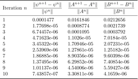
Table 1. Numerical convergence. Iteration n kψ n+1− ψnk kψnk kAn+1− Ank kAnk kBn+1− Bnk kBnk 1 0.0001477 0.0161846 0.0212656 2 1.77698e-05 0.0008774 0.0021739 3 6.74457e-06 0.0001095 0.0003792
4 4.71623e-06 1.1026e-05 7.0184e-05
5 3.45322e-06 1.70946e-05 2.07231e-05
6 2.53969e-06 1.27861e-05 1.25182e-05
7 1.86885e-06 8.90356e-06 9.60398e-06
8 1.37495e-06 6.29852e-06 7.40854e-06
9 1.01137e-06 4.54006e-06 5.59427e-06
10 7.43857e-07 3.30811e-06 4.1659e-06
4. Numerical results
The method detailed in this paper has been implemented in the software Equinox developed in collaboration with the Fusion Department at Cadarache for Tore Supra (see [9, 10, 11]) and JET (Join European Torus). Equinox can be used on the one hand for precise studies in which the computing time is not a limiting factor and on the other hand in a real-time framework.
In table 1, the evolution of the relative residu on ψ, A and B versus the number of iterations is given. It demonstrates numerically the convergence of the algorithm.
If a value ǫ = 10−6 is used as stop condition, the algorithm almost always needs about 5 to
30 iterations to converge. For the finite element mesh of 412 nodes and 762 elements used at Tore Supra the average iteration cost (file access included) is of 0.038 s on a processor Intel(R) Core(Tm)2 Duo T7100 1.80GHz. The expensive operations are the updates of matrices C and Y and the computation of products CK−1and CK−1Y (see Section 3.2). The resolution of the direct problem (Eq. 14) is cheap since the matrix K−1 is stored once for all and does not change
from one iteration to the other. Morevover the resolution of the normal equation (Eq. 17) is also cheap. Each function A and B is decomposed in a basis Φi (which can be chosen to be cubic
B-splines, piecewise linear functions or wavelet scaling functions) of about 5 to 10 functions (depending on the user’s choice). This makes the dimension of the matrix to be inverted at most 20 × 20.
For real-time applications the numerical reconstruction of an equilibrium must not take more than 0.050 to 0.100 s. Therefore in this context it is not possible to let the algorithm fully converge. A maximum number of iterations has to be set (typically 1 or 2 depending on the computer and the size of the mesh). In practice this is not a real problem since our approach is quasi-static. Two successive equilibriums during a pulse are very close and no important differences have been observed between the results of the fully converged algorithm and its real-time version.
Concerning Tikhonov regularization with a real-time constraint it is absolutely not possible to compute the regularization parameter for each equilibrium. Therefore it is kept constant during a pulse. The L-curve method [12] provided a value of approximately 5 × 10⁻⁵.
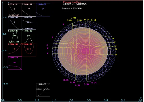
An example of the outputs of Equinox is presented in figure 3. It is a Tore Supra pulse in which magnetic, interferometric and polarimetric measurements on 5 chords are used. One can observe the position of the plasma in the vacuum vessel. Isoflux lines are displayed from the magnetic axis to the boundary. For each active chord, the error between computed and measured
interferometry is given in purple. These errors are less than 1%. The polarimetry errors are given in yellow. They are one order of magnitude larger than for interferometry. Different graphs are plotted on the left of the display. On the first row the identified function A, and corresponding functions p′ and p. On the second row the identified function B and corresponding function f f′. The third row gives the toroidal current density jφ in the equatorial plane and the fourth one
shows the safety factor. Finally on the fifth row the identified ne function is plotted.
Figure 3. Example of Equinox output. See text for details.
References
[1] Grad H and Rubin H 1958 2nd U.N. Conference on the Peaceful uses of Atomic Energy vol 31 (Geneva) pp 190–197
[2] Shafranov V 1958 Soviet Physics JETP 6 1013
[3] Mercier C 1974 The MHD approach to the problem of plasma confinement in closed magnetic configurations Lectures in Plasma Physics (Luxembourg: Commission of the European Communities)
[4] Lao L, Ferron J, Geoebner R, Howl W, St John H, Strait E and Taylor T 1990 Nuclear Fusion 30 1035 [5] Blum J, Lazzaro J, O’Rourke J, Keegan B and Stefan Y 1990 Nuclear Fusion 30 1475
[6] Blum J and Buvat H 1997 IMA Volumes in Mathematics and its Applications, Large Scale Optimization with
applications, Part 1: Optimization in inverse problems and design vol 92 ed Biegler, Coleman, Conn and
Santosa pp 17–36
[7] Tikhonov A and Arsenin V 1977 Solutions of Ill-posed problems (Winston, Washington, D.C.) [8] Ciarlet P 1980 The Finite Element Method For Elliptic Problems (North-Holland)
[9] Bosak K 2001 Real-time numerical identification of plasma in tokamak fusion reactor Master’s thesis University of Wroclaw, Poland URL http://panoramix.ift.uni.wroc.pl/∼bosy/mgr/mgr.pdf
[10] Blum J, Bosak K and Joffrin E 2004 12th ICPP International Congress on plasma physics (Nice) URL http://fr.arxiv.org/abs/physics/0411181
[11] Bosak K, Blum J, Joffrin E and Sartori F 2003 EPS Conference on plasma physics (Saint-Petersbourg) [12] Hansen C 1998 Rank-Deficient and Discrete Ill-Posed Problems: Numerical Aspects of Linear Inversion