The chemodynamics of prograde and retrograde Milky Way stars

HAL Id: insu-03001942

https://hal-insu.archives-ouvertes.fr/insu-03001942

Submitted on 5 Mar 2021

HAL is a multi-disciplinary open access

archive for the deposit and dissemination of

sci-entific research documents, whether they are

pub-lished or not. The documents may come from

teaching and research institutions in France or

abroad, or from public or private research centers.

L’archive ouverte pluridisciplinaire HAL, est

destinée au dépôt et à la diffusion de documents

scientifiques de niveau recherche, publiés ou non,

émanant des établissements d’enseignement et de

recherche français ou étrangers, des laboratoires

publics ou privés.

The chemodynamics of prograde and retrograde Milky

Way stars

Georges Kordopatis, Alejandra Recio-Blanco, Mathias Schultheis, Vanessa Hill

To cite this version:

Georges Kordopatis, Alejandra Recio-Blanco, Mathias Schultheis, Vanessa Hill. The chemodynamics

of prograde and retrograde Milky Way stars. Astronomy and Astrophysics - A&A, EDP Sciences,

2020, 643, pp.A69. �10.1051/0004-6361/202038686�. �insu-03001942�

https://doi.org/10.1051/0004-6361/202038686 c G. Kordopatis et al. 2020

Astronomy

&

Astrophysics

The chemodynamics of prograde and retrograde Milky Way stars

Georges Kordopatis (

Γι ´ωργoς Koρδoπ ´ατης), Alejandra Recio-Blanco, Mathias Schultheis, and Vanessa Hill

e-mail: gkordo@oca.eu

Received 18 June 2020/ Accepted 11 September 2020

ABSTRACT

Context.The accretion history of the Milky Way is still unknown, despite the recent discovery of stellar systems that stand out in terms of their energy-angular momentum space, such as Gaia-Enceladus-Sausage. In particular, it is still unclear how these groups are linked and to what extent they are well-mixed.

Aims.We investigate the similarities and differences in the properties between the prograde and retrograde (counter-rotating) stars and set those results in context by using the properties of Gaia-Enceladus-Sausage, Thamnos/Sequoia, and other suggested accreted populations.

Methods. We used the stellar metallicities of the major large spectroscopic surveys (APOGEE, Gaia-ESO, GALAH, LAMOST, RAVE, SEGUE) in combination with astrometric and photometric data from Gaia’s second data-release. We investigated the presence of radial and vertical metallicity gradients as well as the possible correlations between the azimuthal velocity, vφ, and metallicity,

[M/H], as qualitative indicators of the presence of mixed populations.

Results.We find that a handful of super metal-rich stars exist on retrograde orbits at various distances from the Galactic center and the Galactic plane. We also find that the counter-rotating stars appear to be a well-mixed population, exhibiting radial and vertical metallicity gradients on the order of ∼ − 0.04 dex kpc−1and −0.06 dex kpc−1, respectively, with little (if any) variation when different regions of the Galaxy are probed. The prograde stars show a vφ− [M/H] relation that flattens – and, perhaps, even reverses as a function of distance from the plane. Retrograde samples selected to roughly probe Thamnos and Gaia-Enceladus-Sausage appear to be different populations yet they also appear to be quite linked, as they follow the same trend in terms of the eccentricity versus metallicity space.

Key words. Galaxy: abundances – Galaxy: formation – Galaxy: disk – Galaxy: kinematics and dynamics – Galaxy: stellar content – stars: abundances

1. Introduction

The role that accretion events have played in the evolution of the Milky Way and the quest to find possible remnants that are at the origin of the old disc have been central topics in Galac-tic archaeology for over than five decades (e.g. Eggen et al. 1962; Searle & Zinn 1978; Gilmore & Reid 1983; Chiba & Beers 2000;Gilmore et al. 2002;Wyse et al. 2006;Kordopatis et al. 2011). The advent of the Tycho-Gaia Astrometric Solu-tion (TGAS) catalogue of the European space mission, Gaia (Gaia Collaboration 2016b,a), and, in particular, the second Gaia data release (GDR2, Gaia Collaboration 2018a), have enabled us to measure with much greater accuracy the positions and the 3D velocities of millions of stars in a volume several kilopar-secs wide. Such studies have shed an unprecedented light on the questions cited above.

On the one hand, the discovery of ripples in the Galactic disc has shown that its morphology and characteristics, at all radii, continue to be impacted by external factors (Gaia Collaboration 2018c; Antoja et al. 2018; Laporte et al. 2018, 2019). On the other hand, the discovery of kinematic groups outside the disc, such as the Gaia-Sausage (Belokurov et al. 2018;Myeong et al. 2018a), Gaia-Enceladus (Helmi et al. 2018), Sequoia (Myeong et al. 2019), and Thamnos (Koppelman et al. 2019) are all believed to be remnants of past accretions; however, it is still unclear whether or not they are distinct features and to what extent they might have contributed at the formation of the thick disc or the

inner halo (e.g.Haywood et al. 2018;Fernández-Alvar et al. 2019;

Belokurov et al. 2020).

In that respect, retrograde stars in the Milky Way hold a key place in our understanding of the assembly history of our Galaxy because there is no clear mechanism that could form them exclu-sively in situ. Counter-rotating stars in the halo have been dis-cussed since Majewski (1992), Carney et al. (1996), Carollo et al.(2007),Nissen & Schuster(2010),Majewski et al.(2012). In particular,Majewski(1992) identified, via an investigation of proper motions and a multi-colour analysis of a sample of few hundred stars towards the north Galactic pole, a retrograde rota-tion among stars reaching 5 kpc from the plane.Majewski(1992) reports that they exhibit no radial metallicity gradient, while also stating that this population may be younger, on average, than the dynamically hot metal-poor stars that are closer to the plane. This result was later confirmed byCarney et al.(1996) using a kinematically biased sample of 1500 stars and byCarollo et al.

(2007) using calibration data from 20 000 stars from the Sloan Extension for Galactic Understanding and Exploration (SEGUE,

Yanny et al. 2009).

Nissen & Schuster(2010) carried out a spectroscopic obser-vation at high resolution of a sample of 94 kinematically selected dwarf stars and found that the low-[α/Fe] sequence stars iden-tified in the [α/Fe] vs [Fe/H] plane were mostly counter-rotating targets. According to the authors, some of the low-[α/Fe] sequence stars may have originated from ω Centauri’s globular cluster progenitor (the latter also being on a retrograde

Open Access article,published by EDP Sciences, under the terms of the Creative Commons Attribution License (https://creativecommons.org/licenses/by/4.0),

orbit; see e.g. Dinescu et al. 2002), a hypothesis that has also been suggested byMajewski et al.(2012), using low-resolution (R ∼ 2600) spectra of ∼3000 stars, and by Myeong et al.

(2018b), using a catalogue of ∼62 000 halo stars from a cross-match of Gaia DR1, the SDSS DR 9 (Ahn et al. 2012), and LAMOST DR 3 (Luo et al. 2015) catalogues.

Using the exquisite GDR2 data,Gaia Collaboration(2018b) found that a non-negligible amount of the halo stars in the extended Solar neighbourhood that are somewhat less bounded than the Sun are on retrograde orbits. Compared with cosmo-logical simulations, they conclude that this rate of counter-rotating stars, despite being rare, is not unexpected. Helmi et al. (2018) suggested that they originate from the merger with Gaia-Enceladus, the latter in a slightly counter-rotating orbit with a mass ratio of 4:1 (see also Gallart et al. 2019,

Feuillet et al. 2020).

While the metallicity extent, chemical structure as well as the number of subpopulations that constitute these retrograde stars have already been investigated in previous papers in action-angular momentum space (e.g.Helmi et al. 2018;Myeong et al. 2018a,2019;Koppelman et al. 2019;Feuillet et al. 2020;Naidu et al. 2020), the investigation of the correlation between the stel-lar azimuthal velocity, vφ, and the stellar metallicity, [M/H], or

iron abundance, [Fe/H], can provide an additional insight in this endeavour (e.g.Kordopatis et al. 2013a, for the identification of thick disc stars and characterisation of its properties). The level of correlation between two or more parameters can also highlight the mechanisms that have formed and shaped a stellar population that is being considered.

While this was already visible in previous datasets (see e.g.

Carney et al. 1996), Spagna et al. (2010), Kordopatis et al.

(2011),Lee et al.(2011) isolated the correlation between kine-matics and metallicity for thick disc stars and measured it to be on the order of ∂vφ/∂[M/H] ≈ +50 km s−1dex−1. A mild

nega-tive correlation has also been measured for the chemically identi-fied thin disc stars inRecio-Blanco et al.(2014),Kordopatis et al.

(2017),Allende Prieto et al.(2016). Whereas for the thin disc, this correlation is well-understood as the effect of blurring and churning in the disc (e.g.Sellwood & Binney 2002;Schönrich & Binney 2009;Minchev & Famaey 2010), multiple explanations can be found in the literature concerning the origin of the positive correlation for the thick disc stars. Indeed, it has been suggested that it could either be the signature of the collapse of a primitive gas cloud (e.g.Kordopatis et al. 2017), a signature of inside-out formation and gas re-distribution in the primitive disc (Schönrich & McMillan 2017), or, as recently suggested byMinchev et al.

(2019), a correlation resulting from the superposition of mono-[α/Fe] sub-populations with negative slopes (as in the thin disc). In the latter case, the measured positive correlation is due to the combination of several populations of different ages with differ-ent relative weights and proportions (the so-called Yule-Simpson paradox).

In this paper, we aim to study the chemokinematics of the stars in the Gaia-sphere, with a particular focus on the retrograde targets, in order to identify trends that could shed some light on the formation origins of the thick disc and the origin of those retrograde stars. Section2 describes the dataset used in this analysis. Sections3 and 4 show the spatial metallicity gradients and the correlations between the azimuthal velocity and metallicity for the prograde and retrograde stars, whereas Sect.5 discusses selections prob-ing Gaia-Enceladus-Sausage stars and other accreted popula-tions, selected in the phase-space. Finally, Sect.6 presents our conclusions.

2. Description of the dataset used and the quality cuts applied

We used the distance, velocity, and age catalogue of stars of

Sanders & Das(2018) to select targets from LAMOST (DR3,

Deng et al. 2012), APOGEE (DR14, Abolfathi et al. 2018), RAVE (DR5,Kunder et al. 2017), SEGUE (DR12,Yanny et al. 2009), GALAH (DR2,Buder et al. 2018), and Gaia-ESO (DR3,

Gilmore et al. 2012) surveys.

We applied the quality-flag present in the catalogue to remove all the stars for which the spectroscopic parameters are too far from the isochrones to have reliable distances and ages (i.e. those that do not have the value of flag equal to zero; see

Sanders & Das 2018, for more details). We also removed the RAVE-on (Casey et al. 2017) entries in order to avoid duplicates with RAVE-DR5. As far as the Teff range is concerned, we only

kept the stars between 3500 K and 6800 K in order to avoid too cool or too hot stars for which spectra parameterisation is intrin-sically difficult to obtain and its results uncertain, thus introduc-ing a potential bias1_.

In addition to the filters above, further cuts were required in order to make sure our sample contained only single stars. To achieve this, we cross-matched the sample of stars that fulfil the above criteria with the GDR2 archive, based on the GDR2 sourceid. We extracted the renormalised unit weight error (RUWE) of the targets and discarded the stars with a RUWE greater than 1.2 (suggesting that Gaia’s astrometric solution has not converged appropriately and that the considered stars are potential binaries)2_{, an astrometric excess noise greater than}

1, and, finally, a parallax relative uncertainty (σ$/$) greater than 0.1. The latter filter ensures that what dominates the stel-lar distance estimation is the parallax measurement and not the prior adopted in Sanders & Das (2018). We note that the adopted distances do not take into consideration the zero-point offset reported for GDR2 parallaxes (e.g.Lindegren et al. 2018;

Schönrich et al. 2019), as it has a dependence on the position on the sky, the magnitude, and the colour of the star, which compli-cates an application that does not involve the introduction of fur-ther biases (e.g.Gaia Collaboration 2018a;Arenou et al. 2018). That said, the global effect of this zero point on the velocities and gradients is discussed in the relevant sections below and in greater detail in AppendixA.

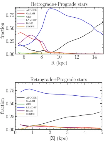
We also discarded the stars that have an uncertainty in metal-licity greater than 0.2 dex, a vφuncertainty greater than 50 km s−1, and a Galactocentric cartesian X position that suggests they are located past the Galactic center (in order to avoid probing entirely different regions of the Galaxy at a given R). Our final work-ing sample was obtained by removwork-ing the inter-survey repeats, using the duplicate keyword in the Sanders & Das (2018) table, which preferentially selects the stars in the order: APOGEE, GALAH, GES, RAVE, LAMOST, and SEGUE (for a comparison between the metallicity, the distance, and the azimuthal velocity for the repeated inter-survey stars, see AppendixB). Eventually, we ended up with 2 419 655 unique stars, out of the 4 906 746 entries in the initial catalogue. The relative fractions of each cat-alogue as a function of the Galactocentric radius, R, and abso-lute distance from the Galactic plane, |Z|, are shown in Fig.1. The cumulative distribution functions of the uncertainties in distance,

1 _{A visual inspection of the Kiel diagram confirmed that stars outside}

this range of Teffshould indeed be removed due to their abnormal

loca-tion in this diagram.

2 _{See https://gea.esac.esa.int/archive/documentation/}

GDR2/Gaia_archive/chap_datamodel/sec_dm_main_tables/ ssec_dm_ruwe.html

6

8

10

12

14

R (kpc)

0.00

0.25

0.50

0.75

fraction

Retrograde+Prograde stars

0

1

2

3

4

5

|Z| (kpc)

0.00

0.25

0.50

0.75

fraction

Retrograde+Prograde stars

Fig. 1. Relative fraction of targets within each survey for the stars

closer than 5 kpc from the Galactic plane after application of the quality cuts described in Sect.2, as a function of the Galactocentric radius, R (top), and as a function of absolute distance from the Galactic plane, |Z| (bottom).

metallicity and vφ, split by individual surveys, are shown in Fig.2.

As anticipated, this figure shows that low-resolution surveys tend to have larger uncertainties in metallicity, and, to some extent, vφ,

yet the uncertainties in distance are mostly driven by the apparent magnitude of the targets.

The stellar orbits were computed using the galpy code (Bovy 2014) with the MWPotential2014 and the action-angle formalism for axisymmetric potentials using Binney (2012)’s Staeckel approximation. To be compatible withSanders & Das

(2018) velocities and priors, we adopted the Solar peculiar veloc-ity fromSchönrich et al.(2010), the velocity of the local stan-dard of rest as VLSR = 240 km s−1, and the Sun’s position equal

to (R, Z)= (8.2, 0.015) kpc.

Once we had our final dataset in hand, we verified again that the metallicities of the stars belonging to the different surveys are roughly on the same scale. This was achieved by visually inspecting that the metallicity distributions close to the Sun’s position (|R− R|< 0.2 kpc, |Z| < 0.2 kpc) peaked at the same

value. The metallicity distributions, shown in Fig. 3, exhibit a good agreement given the distinct selection functions and the discrepancies already identified in Fig.B.1.

3. Radial and vertical metallicity gradients

Figure4shows the Kiel diagram of the prograde (vφ> 0 km s−1, 2 397 183 stars) and retrograde (vφ < 0 km s−1, 22 472 stars) samples. Simply by comparing the two diagrams, especially at

the turn-off and red giant branch (RGB) regions, we can already notice that the age range of the retrograde stars is smaller than that of the prograde stars, yet the large width of the turn-off as well as the width of the RGB, suggests that retrograde stars encompass a range of ages.

Figures5and6show the radial and vertical gradients for the two populations for selected ranges of distances from the plane and Galactocentric radii. The associated measured gradients are reported in Tables1and2, respectively, and are discussed in the following subsections.

3.1. Metallicity gradients for the prograde stars

We find that the radial metallicity gradient of the prograde stars exhibits two regimes. First, in the inner disc (5 ≤ R ≤ 8 kpc), a globally null gradient is present, at all |Z| (0.01 ± 0.002 dex kpc−1 closest to the plane3_{, −0.005 ± 0.005 dex kpc}−1_{in the Z= [1−2]}

kpc bin).

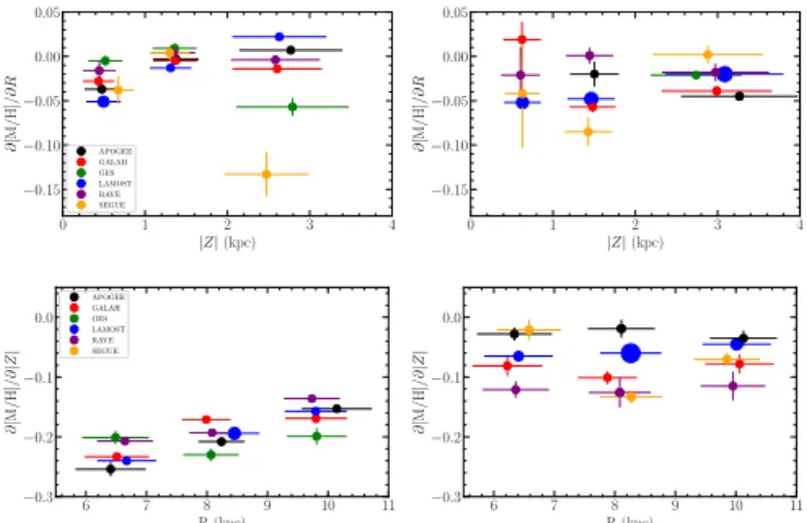
For Galactocentric distances greater than 8 kpc, the metal-licity gradient flattens as one moves further from the plane, regardless of whether we correct for the zero-point offset on the parallaxes (see also Tables A.1 and A.2). For the distances derived without the zero-point correction, the metallicity gradi-ent evgradi-entually reverts from a negative one to a slightly positive one at distances where the thick disc dominates (i.e. |Z| > 2 kpc). This result, first reported inBoeche et al.(2013) using RAVE-DR4 data (Kordopatis et al. 2013a), is not due to small num-ber statistics (as approximately 5 · 104targets are still available at those distances) nor to the non-homogeneity of the consid-ered samples, as the metallicity gradient can also be measured when using LAMOST, APOGEE, RAVE-DR5, and GALAH separately (see top-left panel of Fig.7). The inversion of the gra-dient (or the flattening) can be interpreted as a thick disc that is more centrally concentrated and more metal-poor than the thin disc combined with a thin disc that exhibits a flare at large radii. This result has also been suggested in studies in which the discs have been defined chemically ([α/Fe]-high population for the thick disc and [α/Fe]-low population for the thin disc), such as inBensby et al.(2011),Hayden et al.(2015),Kordopatis et al.

(2015),Minchev et al.(2017),Anders et al.(2017).

Similar to the radial metallicity gradients that exhibit a verti-cal dependency, we find that the vertiverti-cal metallicity gradients of the prograde stars also present a radial dependence, even when individually considering the stars belonging to each survey (see bottom left panel of Fig.7). The gradients we measure for all of the selected stars range from −0.24 dex kpc−1 at the inner disc to −0.17 dex kpc−1at the outer disc. The vertical gradients that are derived for the range 5.3 ≤ R ≤ 9.2 kpc are similar to the gradients previously found in the literature, on the order of −0.2 dex kpc−1to −0.27 dex kpc−1(seeNandakumar et al. 2017, for a comparison between the different surveys), compatible with a mixture of two populations of different scale-heights, namely, hz,thin ∼ 300 pc and hz,thick ∼ 1000 pc (e.g.Gilmore & Reid 1983).

3.2. Metallicity gradients for the retrograde stars

As far as the trends of the retrograde stars are concerned, they are strikingly different than the ones found for the prograde stars.

3 _{The positive gradient for the stars closest to the plane is due to the}

fact that closer to Sun, the average distance of the stars from the Galactic plane is smaller (due to the footprint on the sky of the surveys, trying to avoid the Galactic plane).

0.0 0.5 1.0 1.5 2.0 0.0 0.5 1.0 CDF Prograde APOGEE GALAH GES LAMOST RAVE SEGUE 0.0 0.5 1.0 1.5 2.0 d uncertainty (kpc) 0.0 0.5 1.0 CDF Retrograde 0.00 0.05 0.10 0.15 0.20 0.0 0.5 1.0 Prograde 0.00 0.05 0.10 0.15 0.20 [M/H] uncertainty (dex) 0.0 0.5 1.0 Retrograde 0 20 40 0.0 0.5 1.0 Prograde 0 20 40 vφuncertainty (km s−1) 0.0 0.5 1.0 Retrograde

Fig. 2.Cumulative distribution functions of the uncertainties in line-of-sight distance (left), metallicity (middle), and vφ(right) split by survey

(different colours), and by prograde (top) and retrograde (bottom) populations (as defined in Sect.3).

−0.6 −0.4 −0.2 0.0 0.2 0.4 0.6 [M/H] 0.0 0.5 1.0 1.5 2.0 2.5 3.0 # Solar neighbourhood APOGEE GALAH GES LAMOST RAVEDR5 SEGUE

Fig. 3. Normalised metallicity distributions (obtained using a kernel

density estimation with an Epanechnikov kernel and a smooting param-eter of 0.06 dex) for stars close to the Sun (|R− R| < 0.2 kpc, |Z| <

0.2 kpc), colour-coded by survey. The plot has been truncated at −0.7, in order to better visualise the peak of the distributions. A good agree-ment is found between the different surveys in the sense that they are all peaking at the same value (∼0). We note that the SEGUE distribu-tion contains less than 100 stars (most of them K dwarfs), resulting to a noisier shape.

The radial gradients are always significantly negative, on the order of ∼−0.04 dex kpc−1, with no clear indication of a depen-dency with |Z|, at least up to |Z| ∼ 2 kpc, (even when the surveys are considered individually).

As far as the vertical gradients are concerned, these are much shallower than the ones derived for the prograde stars, yet they are still significant, on the order of ∼ − 0.05 dex kpc−1(see also bottom-right panel of Fig.7for values derived from each survey separately). A mild dependence on the radius might exist, when considering all of the stars simultaneously, in the sense that the outer radial bin seems to have a slightly flatter vertical gradient than the one measured at the inner Galaxy, regardless of the zero-point parallax correction.

The absence, or small dependence, of the vertical metallic-ity gradient variations on the distance from the Galactic center

and of the radial metallicity gradient on the distance from the Galactic plane is compatible with either a well-mixed popula-tion or a single populapopula-tion (coming from e.g. a single accrepopula-tion) that would have a pre-existent metallicity gradient (e.g.Abadi et al. 2003). Further investigation is therefore needed in order to better understand this retrograde population. In the next section, we scrutinise the correlations between vφand the metallicity.

4. Correlations between rotational velocity and metallicity

Figures 8–10 show, for the Solar neighbourhood (R = [7.2−9.2] kpc), the inner Galaxy (R = [5.2−7.2] kpc), and the outer Galaxy (R = [9.2−11.2] kpc), respectively, the median [M/H] for 30 km s−1-wide bins in vφ, where each vφ-bin over-laps by half a step with the previous one. The prograde stars are shown on the right-hand side panels and the retrograde stars on the left-hand side panels. We note that these trends do not change (although they become more noisy due to fewer stars) when only one survey is taken into account at once (which is in agreement withNandakumar et al. 2017, who state that the selec-tion funcselec-tions of the considered surveys do not significantly alter the measured Galactic gradients), nor when the zero-point offset in parallax is corrected for.

We also note that the usual way of plotting the chemokine-matic correlations that can be found in the literature is the oppo-site than the one presented in these figures: commonly, it is vφ

that is marginalised over metallicity-bins. However, by doing so, the tails of the velocity distribution are systematically missed or ignored, which is not what we are looking to do in this study. For this reason, the plots that follow are not obtained in the “usual" way, that is, using vφ= f ([M/H]).

4.1. Trends for the prograde stars

Regarding the prograde stars, we can find the expected and known trends in the disc: close to the plane (purple colours on the right panels of Figs.8–10), stars show a negative correlation down to vφ∼ 180 km s−1(the typical velocity-lag of the thick disc). Then they show a positive correlation for lower angular momenta.

Fig. 4.Kiel diagrams for the stars that fulfilled our quality criteria for the prograde (left) and retrograde (right) populations, colour-coded by azimuthal velocity vφ.

6

8

10

12

14

R (kpc)

−1.5

−1.0

−0.5

0.0

[M

/H]

Fig. 5.Radial gradients for the prograde stars (in black) and the

retro-grade stars (in red). Solid, dashed, and dotted lines correspond to selec-tions for 0.2 ≤ |Z| < 1 kpc, 1 ≤ |Z| < 2 kpc, and 2 ≤ |Z| < 4.5 kpc, respectively. Error bars are computed as σ/√N.

0

1

2

3

4

5

|Z| (kpc)

−1.5

−1.0

−0.5

0.0

[M

/H]

Fig. 6.Vertical gradients for the prograde stars (in black) and the

retro-grade stars (in red). Solid, dashed, and dotted lines correspond to selec-tions for 7.2 ≤ R < 8.2 kpc, 5.2 ≤ R < 7.2 kpc, and 9.2 ≤ R < 11.2 kpc, respectively.

The negative correlation, typically found for the chemically defined thin disc stars (e.g.Lee et al. 2011;Recio-Blanco et al. 2014;Allende Prieto et al. 2016;Kordopatis et al. 2017) is due

Table 1. Measured Galactocentric radial gradients in the R = [5−15] kpc range.

|Z|-range Prograde Retrograde (kpc) (dex kpc−1) (dex kpc−1) [0.2−1.0] −0.037 ± 0.003 −0.041 ± 0.008 [1.0−2.0] −0.004 ± 0.002 −0.048 ± 0.005 [2.0−4.5] 0.012 ± 0.003 −0.028 ± 0.003

Table 2. Measured vertical gradients relative to the Galactic plane in the range |Z|= [0−5] kpc.

R-range Prograde Retrograde (kpc) (dex kpc−1_{) (dex kpc}−1₎

[5.2−7.2] −0.236 ± 0.007 −0.071 ± 0.007 [7.2−9.2] −0.202 ± 0.006 −0.062 ± 0.009 [9.2−11.2] −0.171 ± 0.005 −0.043 ± 0.007

to the blurring of the stellar orbits: older thin disc stars have a higher eccentricity than young stars via more Lindblad reso-nances with the spiral arms; this eventually allows them to visit radii that are far from their birth radius (Lynden-Bell & Kalnajs 1972). As a consequence, old outer thin disc stars can reach the solar neighbourhood at their pericentre, hence with velocities lower than the local standard of rest (LSR), and the inner thin disc stars can reach the solar neighbourhood at their apocentre, hence with velocities higher than the LSR. Because of the radial metallicity gradient in the thin disc, stars that are more metal-rich than the locally born stars tend to move faster than the LSR, and the stars that are more metal-poor than the locally born stars will tend to move slower than the LSR. Comparing the metallicities at which the inflexion happens in Figs.8–10, we can notice that it shifts from super-solar metallicities at the inner disc to sub-solar metallicities at our outer disc sample, which is as expected for a disc with a negative radial metallicity gradient.

The positive correlation that we find for stars with vφ .

0 1 2 3 4 |Z| (kpc) −0.15 −0.10 −0.05 0.00 0.05 ∂ [M /H] /∂ R APOGEE GALAH GES LAMOST RAVE SEGUE 0 1 2 3 4 |Z| (kpc) −0.15 −0.10 −0.05 0.00 0.05 ∂ [M /H] /∂ R 6 7 8 9 10 11 R (kpc) −0.3 −0.2 −0.1 0.0 ∂ [M /H] /∂ |Z | APOGEE GALAH GES LAMOST RAVE SEGUE 6 7 8 9 10 11 R (kpc) −0.3 −0.2 −0.1 0.0 ∂ [M /H] /∂ |Z |

Fig. 7.Radial (top) and vertical (bottom) metallicity gradients for the

prograde (left) and retrograde (right) samples, split by survey. The ver-tical error bars correspond to the uncertainty of the fit of the gradient, whereas the horizontal error bar represents the dispersion in |Z| or R, respectively, where the gradient was measured. The size of the dots is a visual aid proportional (within each panel) to the number of stars each survey contains in the considered distance-bin.

Spagna et al. 2010;Kordopatis et al. 2011,2017;Lee et al. 2011;

Recio-Blanco et al. 2014;Re Fiorentin et al. 2019) is often used as an argument against radial migration in the thick disc. We note, however, that Minchev et al.(2019) suggested that this correlation may be due to the superposition of stars of different ages, each mono-age population itself having a negative corre-lation (the so-called Yule-Simpson effect). The precision of the ages available for our sample does not allow us to either support or reject this statement.

That said, we find that the trends become flatter as we move farther from the plane. Eventually, for 6 < |Z| < 10 kpc (or even |Z| > 4 kpc, when the zero-point offset in parallax is taken into account), that is, where the canonical thick disc still represents a significant fraction of the stars (assuming a scale-height of 1 kpc and a local normalisation of ∼0.1), the trends seem to become negative for all of the stars over all the vφ-range (i.e. even at large

velocities where the ratio canonical thick disc or canonical halo is high) and at all Galactocentric radii. This result is compatible withMinchev et al.(2019) and could potentially suggest that the thick disc stars far from the plane and the inner halo might be one single mono-age population. To our knowledge, this flattening trend has not been identified in any previous study.

4.2. Retrograde stars

Unlike the prograde stars, all of the retrograde stars seem to exhibit similar behaviour at any distance from the plane and any distance from the Galactic centre. The correlation is always positive, on the order of ∼25−30 km s−1dex−1, again suggest-ing that the probed population is well-mixed at all R (one would otherwise expect different trends). However, the retrograde sam-ple contains, rather unexpectedly, super-solar metallicity (SMR) stars (see for instance Figs. A.2 and A.3 as well as Fig. 8, left panel, around vφ ∼ −325 km s−1). Although only ∼600 of them (∼300 when the zero-point offset in parallax is taken into account, observed mostly by the APOGEE, LAMOST, and RAVE surveys), they show an inverse (i.e. negative) correlation with metallicity, similar to the thin disc prograde stars. These SMR stars are located at all Galactic sky coordinates (`, b), with 50 per cent of them being closer than 1 kpc from the Galactic

plane, and reaching distances up to |Z| ∼ 6−7 kpc. They are also seen in both the inner and the outer Galaxy (up to R ∼ 15 kpc). Interestingly, when the zero-point offset in parallaxes is not taken into account, 20% of the retrograde stars are located in the bulge region, that is, between 1 < R < 2.5 kpc, but the latter sample becomes prograde when correcting for the zero point (also see the plots in Figs.A.2andA.3).

We cross-matched our retrograde sample with the APOGEE-DR16 catalogue (Ahumada et al. 2020) and out of the 1197 stars which have a reliable abundance determination4, we find that 18 have [M/H] > 0 (see Fig.11)5_{. A specific investigation of the}

stellar spectra belonging to the APOGEE, LAMOST and RAVE surveys will be performed in future papers with the aim of con-firming whether those SMR retrograde stars are indeed as metal-rich as suggested by theSanders & Das(2018) catalogue. We show, nevertheless, in Fig.12, the APOGEE DR16 spectra and their best-fit templates for five of those SMR retrograde targets as a preview of the study that will follow, also indicating that these stars have a good parameterisation.

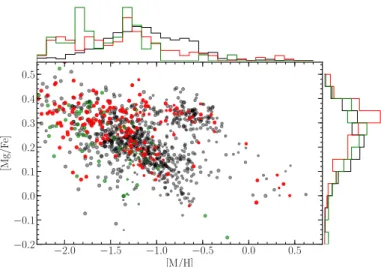
Recently, Fragkoudi et al. (2020),Belokurov et al. (2020) andGrand et al.(2020) revived the idea that the thick disc may have formed after a violent gas-rich merger (e.g. Brook et al. 2004). In this context, because of the compressible nature of the gas, some of the newborn stars could have been formed on counter-rotating or radial orbits. The time and mass of this gas-rich merger, according toGrand et al.(2020), could be then inferred from the properties and the fraction of the locally born retrograde stars. Figure11shows the magnesium abundance as a function of metallicity for all of the retrograde stars in the APOGEE DR16 sample. We can see from this figure two chem-ical sequences starting at [M/H] & −1.5: a high-α, typically associated with stars born in situ, and a low-α, associated with accreted populations (e.g.Nissen & Schuster 2010). Whereas the majority of the counter-rotating stars are located in the low−α sequence, a non-negligible fraction of them, extending up to super-solar metallicities, are on the high-α sequence, indicating that they are possibly born locally. As we do not know the selec-tion funcselec-tion of our sample, we cannot draw conclusions on their relative proportions. However, the fact that they are slightly α-enhanced, even for [M/H] > 0, corroborates to the fact that they were likely born from in situ material.

According toHelmi(2020),Naidu et al.(2020), the largest fraction of retrograde low-α stars belong to Gaia-Enceladus-Sausage, especially at large distances from the plane. In the scenario where Gaia-Enceladus-Sausage was a massive merger (with a mass-ratio of 4:1), this could imply that such a massive galaxy would have an internal metallicity gradient and puffed-up the Galactic disc that was present at the time of the merger. The low-metallicity accreted stars from such a merger would there-fore be deposed first, on high eccentricity, and the metal-rich stars (formed close to the center of the accreted galaxy) would be deposited on more circular orbits due to dynamical friction (e.g.

Koppelman et al. 2020). In the next section, we investigate more closely the case of Gaia-Enceladus-Sausage and try to identify differences with the other retrograde stars and groups of accreted stars, as identified recently in the literature.

4 _{Throughout the paper, we remove from the APOGEE DR16}

catalogue those stars with a signal-to-noise ratio (S/N) lower than 60, as well as those flagged with the following keywords: BAD_PIXELS, BAD_RV_COMBINATION, LOW_SNR, PERSIST_HIGH, SUSPECT_BROAD_LINES, VERY_BRIGHT_NEIGHBOR, NO_ASPCAP_ RESULT, STAR_BAD, SN_BAD, STAR_BAD, CHI2_BAD, COLORTE_BAD.

5 _{When taking into account the zero point of the parallax, we end up}

0 100 200 300 |vφ| (km s−1) −2.0 −1.5 −1.0 −0.5 0.0 0.5 [M/H] [0;1.5] [1.5;3] [3;6] [6;10] retrograde 0 100 200 300 vφ(km s−1) [0;0.5] [0.5;1] [1;2] [2;3] [3;4] [4;6] [6;10] prograde

Fig. 8.vφvs [M/H] for the stars in the Solar cylinder (R= [7.2−9.2] kpc). Different colours correspond to different distances from the Galactic

plane (darker colours correspond to the closest to the plane, yellow colours to the farthest distances), the range in kpc being reported at the lower-left corner of each plot. The vertical dashed line is at VLSR and horizontal dashed line is at solar metallicity. Vertical error bars correspond to

σ[M/H]/

√

N, where N is the number of stars in a given bin and σ[M/H]is the standard deviation of the metallicity inside that bin.

0 100 200 300 |vφ| (km s−1) −2.0 −1.5 −1.0 −0.5 0.0 0.5 [M/H] [0;1.5] [1.5;3] [3;6] [6;10] retrograde 0 100 200 300 vφ(km s−1) [0;0.5] [0.5;1] [1;2] [2;3] [3;4] [4;6] [6;10] prograde

Fig. 9.Same as Fig.8, but for the inner Galaxy (R= [5.2−7.2] kpc).

0 100 200 300 |vφ| (km s−1) −2.0 −1.5 −1.0 −0.5 0.0 0.5 [M/H] [0;1.5] [1.5;3] [3;6] [6;10] retrograde 0 100 200 300 vφ(km s−1) [0;0.5] [0.5;1] [1;2] [2;3] [3;4] [4;6] [6;10] prograde

Fig. 10.Same as Fig.8, but for the outer Galaxy (R= [9.2−11.2] kpc).

5. Gaia-Enceladus-Sausage, Thamnos/Sequoia,

ω

In what follows, we define three sub-samples of counter-rotating stars.

First, we labelled, as “Gaia-Enceladus-Sausage” the targets fulfilling the quality criteria presented in Sect. 2 and having LZ < 0 kpc km s−1 and vφ > −200 km s−1 as well as e > 0.65

(16 283 out of the 22 472 counter-rotating stars, LAMOST and

APOGEE targets encompassing 56.4 and 16.1 per cent of the tar-gets, respectively). This selection is somewhat compatible with remnants of a counter-rotating merger of initial inclination of approximately 30 deg (seeHelmi 2020, Sect. 4.2.1) but we stress that it ignores the prograde counter-part of the merger remnants and is likely contaminated by other accreted populations (see for exampleFeuillet et al. 2020). Therefore, our sample should not be directly compared with other Enceladus or Gaia-Sausage samples in the literature.

−2.0 −1.5 −1.0 −0.5 0.0 0.5 [M/H] −0.2 −0.1 0.0 0.1 0.2 0.3 0.4 0.5 [Mg/F e]

Fig. 11.Scatter plot of magnesium abundance as a function of

metal-licity for the retrograde stars in the APOGEE-DR16 catalogue and marginalised normalised histograms. Black, red, and green points and histograms correspond to counter-rotating stars that we labelled “Gaia-Enceladus-Sausage”, “Thamnos”, and “other”, respectively (the criteria for selecting those stars are described in Sect.5). The sizes of the points are indicative and correspond to the estimated ages fromSanders & Das (2018); we note, however, that the majority of these stars are giants and, hence, their ages are unreliable.

We also selected stars probing the chemically and dynami-cally peculiar population identified byKoppelman et al.(2019) and dubbed “Thamnos”, the targets fulfilling the previous qual-ity criteria and having LZ < 0 kpc km s−1, e < 0.65, as well as

vφ> −200 km s−1(4007 stars, LAMOST and APOGEE encom-passing 52.1 and 19.2 per cent of the targets, respectively), that is, the stars having similar angular momentum and vφ as our “Gaia-Enceladus-Sausage” sample, but having low eccentrici-ties. Despite being still unclear if “Thamnos” is part of the low-energy tail of Sequoia (see Myeong et al. 2019; Naidu et al. 2020), in what follows we nevertheless labelled this sample “Thamnos” as the majority of Sequoia stars are on higher energy orbits.

Finally, all the other retrograde stars that are not “Gaia-Enceladus-Sausage” nor “Thamnos”, with Lz < 0 kpc km s−1,

are labelled in what follows as "other" (1 461 stars, LAMOST, RAVE and APOGEE encompassing 58.1, 13.6, and 13.1 per cent of the targets, respectively). It is noteworthy that this category comprises, “Sequoia” stars as well as other sub-populations (see e.g.Naidu et al. 2020).

Figures13 and14show the radial and vertical metallicity gradients for those three samples. We did not separate them into different vertical or radial ranges, as we did in Sect. 3.2, since we found that the gradients for the retrograde stars are not particularly dependent on spatial cuts. We find that the “Gaia-Enceladus-Sausage” sample is globally more metal-rich than the “Thamnos” sample (in agreement withKoppelman et al. 2019;

Mackereth et al. 2019) and that the two former samples are, in turn, more metal-rich than the “other” counter-rotating sample in our sample.

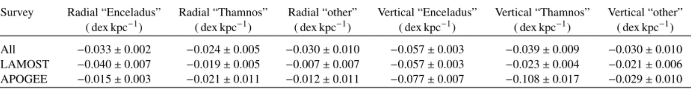
When considering all of the surveys simultaneously, the radial and vertical metallicity gradients that we measure for “Gaia-Enceladus-Sausage”, “Thamnos”, and the “other” sub-samples are similar, within 1σ and 2σ, respectively (see Table3), yet this result should be taken with a grain of salt as it is not necessarily corroborated when considering LAMOST or

APOGEE targets separately (maybe due to small number statis-tics or different volume coverage).

This lack of evidence of difference in the metallicity gra-dients, other than the zero-point offset, between each of the counter-rotating sub-samples, made us investigate how the metallicity changed as a function of the eccentricity. Results are shown in Fig.15. Strikingly, we find that “Gaia-Enceladus-Sausage” and “Thamnos” samples follow the same trend, as opposed to the “other” subsample, which appears to show no variation of metallicity as a function of the eccentricity (a result that is also found when separating the targets per survey). This trend seems to favour the fact that the “Thamnos” and “Gaia-Enceladus-Sausage” samples are strongly linked, yet the ques-tion remains about whether they originate from the same parent population.

The [Mg/Fe] − [M/H] plot coming from the APOGEE-DR16 data (Fig.11) shows not only that our “Gaia-Enceladus-Sausage” and “Thamnos” samples are mixed populations, containing both high-α and low-α stars, but also that they exhibit different distributions in both the metallicity space and the [Mg/Fe] space (see coloured dots and histograms). The two sample Kolmogorov-Smirnov tests of the metallicity and [Mg/Fe] between the “Gaia-Enceladus-Sausage” and “Tham-nos” samples strongly suggest that the two samples cannot have been drawn from the same underlying distribution, with p-values always lower than 10−7, even when decomposed into radial and vertical spatial bins.

Finally, we also explored the possibility of having a signif-icant amount of stars belonging to the retrograde (and pecu-liar on many aspects) globular cluster ωCentauri (e.g.Dinescu 2002;Morrison et al. 2009;Nissen & Schuster 2010;Majewski et al. 2012;Myeong et al. 2018b). For this purpose, we visually investigated the [Na/Fe]-[O/Fe] space for indications of an anti-correlation between the Na abundance and the O one, indicative of the one found in ωCen (e.g.,Johnson & Pilachowski 2010;

Gratton et al. 2011;Marino et al. 2011). Figure16shows no clear indication of anything of the sort for either one of the three sub-samples, suggesting that, globally, our sample of retrograde stars does not contain any obvious sub-population of stars stripped from the ωCen progenitor. We note, however, as remarked by

Zasowski et al. (2019), that sodium abundances in APOGEE exhibit a large scatter compared to the published uncertainties, partly due to the presence of strong telluric absorptions close to the Na lines. Therefore, firmer conclusions on this topic might require a more in-depth investigation of the abundance patterns of APOGEE, which is beyond the scope of this paper.

6. Discussion and conclusions

The merger-tree of the Milky Way is a matter of vivid debate. Despite the recent discoveries of many over-densities in the action-energy space in the extended Solar neighbourhood, it is still rather unclear how these populations relate to each other, or to what extent they are well-mixed within the Galaxy. In this paper, we use a compiled catalogue of the metallicities and velocities of more than 4 million stars from Sanders & Das

(2018) to investigate the chemical gradients and the chemo-dynamics of the counter-rotating stars, while also performing similar analyses for the prograde stars. This parallel analysis allowed us to highlight the differences between the two popula-tions and also to confirm that our analysis method returned sound results.

0.50 0.75 1.00 1.25 Teff: 5789; log g: 4.3; [M/H]: 0.08±0.01 1291589166619330048 vφ: -97± 4km s−1 0.50 0.75 1.00 1.25 Teff: 4803; log g: 3.4; [M/H]: 0.18±0.01 2608825739033972224 vφ: -24± 32km s−1 0.50 0.75 1.00 1.25 Teff: 4442; log g: 2.7; [M/H]: 0.4±0.0 1393145901715973120 vφ: -42± 6km s−1 0.50 0.75 1.00 1.25 Teff: 4074; log g: 2.2; [M/H]: 0.62±0.01 4598550672703820288 vφ: -19± 2km s−1 16000 16050 16100 16150 16200 16250 λ (˚A) 0.50 0.75 1.00 1.25 Teff: 3744; log g: 1.3; [M/H]: 0.38±0.01 4050874168537845760 vφ: -107± 46km s−1

Fig. 12.APOGEE DR16 spectra (in a selected arbitrary wavelength range, in black) and best-fit templates (in red) for five of the super-solar

metallicity retrograde stars in our sample. The Gaia sourceid is reported at the top-right corner and the atmospheric parameters of the stars, as well as their azimuthal velocity, vφ, at the top-left corner.

Our main results can be summarised as follows:

– We determined that stars on prograde orbits show a vφ−

[M/H] relation that flattens – and perhaps even reverses as a function of distance from the plane. To our knowledge, this trend has not yet been reported in the literature.

– We found a super-solar metallicity counter-rotating popula-tion over a large range of radii and distances from the plane (|Z| ∼ 5−6 kpc and R ∼ 15 kpc).

– Retrograde stars exhibit vertical and radial metallicity gradi-ents that are similar at all probed radii and distances from the Galactic plane, respectively (∂[M/H]/∂R ≈ −0.04 dex kpc−1 and ∂[M/H]/∂|Z| ≈ −0.06 dex kpc−1).

– The correlation between vφand the metallicity for the

retro-grade stars also seem to be similar everywhere in the Galaxy. – Samples roughly probing “Gaia-Enceladus-Sausage” and “Thamnos” (or Sequoia’s low-energy tail) show similar metallicity gradients but different metallicity and [α/Fe] dis-tributions. Despite being truncated and likely contaminated samples, we find that they are following the exact same

sequence of metallicity versus eccentricity. Other counter-rotating stars with lower vφdo not follow the same sequence.

– Counter-rotating stars do not show any striking anti-correlations in [Na/Fe] versus [O/Fe] chemical space, sug-gesting that our sample does not contain many ωCen stars. We investigated potential biases due to parallax zero-point o ff-sets or the inhomogeneity of the survey metallicities in order to make sure that the results of our analysis are robust. Globally, a correction of the parallax zero point affects mainly the ret-rograde stars, increasing their velocities and, hence, decreasing the sample-size of this population. Our conclusions, however, remain robust as they do not rely on the absolute densities of the populations. The different zero points in metallicity between the surveys do not alter our conclusions either. Indeed, where, for example, the absolute values of the metallicity gradients might differ if a specific survey is used instead of another, the global trends remain unchanged. That said, we stress that additional biases might still exist due to the different quality cuts that we applied to our input catalogue. These are difficult to quantify

6

8

10

12

14

R (kpc)

−2.0

−1.5

−1.0

−0.5

[M

/H]

Fig. 13. Radial gradients for the “Gaia-Enceladus-Sausage” sample

(black), the “Thamnos” sample (red), and the “other” retrograde stars (green). The criteria for selecting those stars are described in Sect.5. The gradient for all of the retrograde stars considered simultaneously is shown in yellow.

0

2

4

6

|Z| (kpc)

−2.0

−1.5

−1.0

−0.5

[M

/H]

Fig. 14.Vertical gradients for the “Gaia-Enceladus-Sausage” sample

(black), the “Thamnos” sample (red), and the “other” retrograde sample (green). The gradient for all of the retrograde stars considered simulta-neously is shown in yellow.

(e.g. the effect of filtering for the stars with large uncertainty in metallicity), still, we present a brief discussion in AppendixC.

From the points above, the following picture can be drawn. The flattening (or inversion of sign, from positive to negative) of the correlation of vφ with metallicity for the prograde stars

far from the plane may suggest, in agreement with other studies, that the inner halo and the thick disc far from the plane may be populations that share a common past. Indeed, it is believed that mono-age disc populations have intrinsically negative vφ−[M/H]

correlations (Minchev et al. 2019). Hence, going from a positive correlation for the thick disc stars close to the plane to a negative (or flat) one for the stars at large distances from it, where the probed population is a mixture of thick disc and halo, would indicate that the targeted population has a smaller age range.

One point that is worth mentioning here relates to recent results, for example, from Haywood et al. (2018), Fernández-Alvar et al.(2019),Myeong et al.(2019),Di Matteo et al.(2019),

Gallart et al. (2019),Belokurov et al.(2020), who revived the idea that the low-angular momentum thick disc might be made up of stars from the proto-disc that are now part of the inner halo after having been heated by a major past accretion (see also, Gilmore et al. 2002; Wyse et al. 2006;Kordopatis et al. 2013b). In particular, using the same input catalogue as we have in this work, Belokurov et al. (2020) identified a small, yet non-negligible, prograde population of intermediate metallicity

([M/H]& −0.7) with low angular momentum (vφ. 100 km s−1), which they have dubbed “the Splash”. These stars are found to be slightly younger than the accreted ones from the last major merger (i.e. Gaia-Enceladus-Sausage) and with a different star-formation history than the latter. These aspects led these authors to suggest that the Splash stars were born locally in the pro-todisc and have had their orbits altered by this massive accretion (see, however, Amarante et al. 2020, for an alternative expla-nation). Our analysis, in selecting each time only the prograde or the retrograde stars, unavoidably dilutes the signature of the Splash with either the thick disc or the halo and Gaia-Enceladus-Sausage targets. However, investigating Figs. 8–10, at around 100 . vφ . 150 km s−1 (whereBelokurov et al. 2020, suggest that there is the overlap between the Splash and the disc), we do not see any peculiarities in the trend other than the well-known change of behaviour in the vφ− [M/H] space, going from an

anti-correlation to a positive correlation.

As far as the counter-rotating stars are concerned, we find that more retrograde targets are also, on average, more metal-poor. The lack of spatial changes in the metallicity gradients, or in the vφ − [M/H] correlations, within the probed volume (5.2 < R < 11.2 kpc and |Z| < 10 kpc), indicate that the counter-rotating stars are remarkably well-mixed. This is in line with, for example,Deason et al.(2018),Helmi(2020) (and with hints of this already discussed inWatkins et al. 2009;Deason et al. 2013) suggesting that the orbital turning points (i.e. shells) of Gaia-Enceladus-Sausage are at a distance of ∼20 kpc, that is, outside the volume that we investigate here. Our results expand upon this, as they show that none of the shells of Gaia-Enceladus-Sausage, Thamnos, Sequoia, or any other accreted population that could compose the retrograde stars, is within 10−12 kpc from the Sun.

Amongst the counter-rotating stars, the samples we dub “Thamnos” and “Gaia-Enceladus-Sausage” seem to compose two different populations that are, nevertheless, also somehow linked. Indeed, we find that the “Thamnos” sample is more metal-poor than the “Gaia-Enceladus-Sausage” one and on more circular orbits. However, it is striking to observe that they fol-low the same trend in the metallicity-eccentricity space. This trend cannot be explained simply by the presence of intrin-sic metallicity gradients within a common progenitor of Gaia-Enceladus-Sausage and Thamnos/Sequoia. Indeed, despite the initial mass estimates of Gaia-Enceladus-Sausage found in the literature, ranging from 6 · 108 _{to 5 · 10}9_M

(e.g.Helmi et al.

2018;Myeong et al. 2019;Kruijssen et al. 2019;Mackereth et al. 2019;Fattahi et al. 2019;Feuillet et al. 2020), which could lead to such internal radial metallicity gradients, it is unclear how a counter-rotating accretion with an angle of ∼30 deg (seeHelmi 2020) would deposit its most metal-rich stars, which would oth-erwise be expected to be present at the innermost regions of the progenitor at the highest eccentricities.

We believe that the key to understanding the effect of the past accretions on the properties of the thick disc is the super-solar metallicity counter-rotating population that we identified in our sample. These stars, if proven to really exist, could have been formed from local gas at the moment of the accretion with the Gaia-Enceladus-Sausage progenitor (seeMaiolino et al. 2017; Gallagher et al. 2019, for star formation activity within galactic outflows). This population would therefore offer us an undeniable sample of locally born retrograde stars in order to precisely date and weigh this merger (see,Grand et al. 2020). The Gaia data release 3, which will become public at the end of 2020, will first confirm whether these peculiar stars are indeed counter-rotating. Then, future large spectroscopic surveys such

Table 3. Measured radial and vertical metallicity gradients for the “Gaia-Enceladus-Sausage”, “Thamnos”, and “other” counter-rotating samples.

Survey Radial “Enceladus” Radial “Thamnos” Radial “other” Vertical “Enceladus” Vertical “Thamnos” Vertical “other”

( dex kpc−1_{) ( dex kpc}−1_{) ( dex kpc}−1_{) ( dex kpc}−1_{) ( dex kpc}−1_{) ( dex kpc}−1₎

All −0.033 ± 0.002 −0.024 ± 0.005 −0.030 ± 0.010 −0.057 ± 0.003 −0.039 ± 0.009 −0.030 ± 0.010 LAMOST −0.040 ± 0.007 −0.019 ± 0.005 −0.007 ± 0.007 −0.057 ± 0.003 −0.023 ± 0.004 −0.021 ± 0.006 APOGEE −0.015 ± 0.003 −0.021 ± 0.011 −0.012 ± 0.011 −0.077 ± 0.007 −0.108 ± 0.017 −0.029 ± 0.010

0.0

0.2

0.4

0.6

0.8

1.0

eccentricity

−2.0

−1.5

−1.0

−0.5

[M

/H]

Fig. 15.Eccentricity gradients for the “Gaia-Enceladus-Sausage”

sam-ple (black), the “Thamnos” samsam-ple (red), and the “other” retrograde stars (green). The gradient for all of the retrograde stars considered simultaneously is shown in yellow.

−0.50 −0.25 0.00 0.25 0.50 0.75 1.00 [O/Fe] −1.5 −1.0 −0.5 0.0 0.5 1.0 [Na/F e]

Fig. 16.Same as Fig. 11but for sodium abundance as a function of

oxygen for the retrograde stars in the APOGEE-DR16 catalogue.

as WEAVE (Dalton et al. 2018) or 4MOST (de Jong et al. 2019) will allow us to verify the chemical composition of these stars, investigate them in more dimensions of the chemical space, and, eventually, to better understand their link with the rest of the galactic populations.

Acknowledgements. We thank the anonymous referee for their useful feedback

that helped improving the quality of this paper. This work has made use of

data from the European Space Agency (ESA) mission Gaia (https://www.

cosmos.esa.int/gaia), processed by the Gaia Data Processing and

Anal-ysis Consortium (DPAC,https://www.cosmos.esa.int/web/gaia/dpac/

consortium). Funding for the DPAC has been provided by national institutions,

in particular the institutions participating in the Gaia Multilateral Agreement.

This research made use of Astropy (http://www.astropy.org), a

community-developed core Python package for Astronomy (Astropy Collaboration 2013,

2018). This work was supported by the Programme National Cosmology et

Galaxies (PNCG) of CNRS/INSU with INP and IN2P3, co-funded by CEA and

CNES and ANR 14-CE33-014-01. GK acknowledges support from OCA and Lagrange BQR. Jason Sanders and Patrick de Laverny are warmly thanked for

useful discussions regarding the catalogue used in this work and the quality cri-teria to apply.

References

Abadi, M. G., Navarro, J. F., Steinmetz, M., & Eke, V. R. 2003,ApJ, 597, 21

Abolfathi, B., Aguado, D. S., Aguilar, G., et al. 2018,ApJS, 235, 42

Ahn, C. P., Alexandroff, R., Allende Prieto, C., et al. 2012,ApJS, 203, 21

Ahumada, R., Prieto, C. A., Almeida, A., et al. 2020,ApJS, 249, 3

Allende Prieto, C., Kawata, D., & Cropper, M. 2016,A&A, 596, A98

Amarante, J. A. S., Beraldo e Silva, L., Debattista, V. P., & Smith, M. C. 2020,

ApJ, 891, L30

Anders, F., Chiappini, C., Minchev, I., et al. 2017,A&A, 600, A70

Antoja, T., Helmi, A., Romero-Gómez, M., et al. 2018,Nature, 561, 360

Arenou, F., Luri, X., Babusiaux, C., et al. 2018,A&A, 616, A17

Astropy Collaboration (Robitaille, T. P., et al.) 2013,A&A, 558, A33

Astropy Collaboration (Price-Whelan, A. M., et al.) 2018,AJ, 156, 123

Belokurov, V., Erkal, D., Evans, N. W., Koposov, S. E., & Deason, A. J. 2018,

MNRAS, 478, 611

Belokurov, V., Sanders, J. L., Fattahi, A., et al. 2020,MNRAS, 494, 3880

Bensby, T., Alves-Brito, A., Oey, M. S., Yong, D., & Meléndez, J. 2011,ApJ,

735, L46

Binney, J. 2012,MNRAS, 426, 1324

Boeche, C., Chiappini, C., Minchev, I., et al. 2013,A&A, 553, A19

Bovy, J. 2014,Galpy: Galactic Dynamics Package(Astrophysics Source Code

Library)

Brook, C. B., Kawata, D., Gibson, B. K., & Freeman, K. C. 2004,ApJ, 612, 894

Buder, S., Asplund, M., Duong, L., et al. 2018,MNRAS, 478, 4513

Carney, B. W., Laird, J. B., Latham, D. W., & Aguilar, L. A. 1996,AJ, 112, 668

Carollo, D., Beers, T. C., Lee, Y. S., et al. 2007,Nature, 450, 1020

Casey, A. R., Hawkins, K., Hogg, D. W., et al. 2017,ApJ, 840, 59

Chiba, M., & Beers, T. C. 2000,AJ, 119, 2843

Dalton, G., Trager, S., Abrams, D. C., et al. 2018,SPIE Conf. Ser., 10702,

107021B

Deason, A. J., Belokurov, V., Evans, N. W., & Johnston, K. V. 2013,ApJ, 763,

113

Deason, A. J., Belokurov, V., Koposov, S. E., & Lancaster, L. 2018,ApJ, 862,

L1

de Jong, R. S., Agertz, O., Berbel, A. A., et al. 2019,Messenger, 175, 3

Deng, L.-C., Newberg, H. J., Liu, C., et al. 2012,Res. Astron. Astrophys., 12,

735

Di Matteo, P., Haywood, M., Lehnert, M. D., et al. 2019,A&A, 632, A4

Dinescu, D. I. 2002, in Omega Centauri, A Unique Window into Astrophysics,

eds. F. van Leeuwen, J. D. Hughes, & G. Piotto,ASP Conf. Ser., 265, 365

Dinescu, D. I., Majewski, S. R., Girard, T. M., et al. 2002,ApJ, 575, L67

Eggen, O. J., Lynden-Bell, D., & Sandage, A. R. 1962,ApJ, 136, 748

Fattahi, A., Belokurov, V., Deason, A. J., et al. 2019,MNRAS, 484, 4471

Fernández-Alvar, E., Tissera, P. B., Carigi, L., et al. 2019,MNRAS, 485, 1745

Feuillet, D. K., Feltzing, S., Sahlholdt, C. L., & Casagrande, L. 2020,MNRAS,

497, 109

Fragkoudi, F., Grand, R. J. J., Pakmor, R., et al. 2020,MNRAS, 494, 5936

Gaia Collaboration (Prusti, T., et al.) 2016a,A&A, 595, A1

Gaia Collaboration (Brown, A. G. A., et al.) 2016b,A&A, 595, A2

Gaia Collaboration(Brown, A. G. A., et al.) 2018a,A&A, 616, A1

Gaia Collaboration (Katz, D., et al.) 2018b,A&A, 616, A11

Gaia Collaboration (Helmi, A., et al.) 2018c,A&A, 616, A12

Gallagher, R., Maiolino, R., Belfiore, F., et al. 2019,MNRAS, 485, 3409

Gallart, C., Bernard, E. J., Brook, C. B., et al. 2019,Nat. Astron., 3, 932

Gilmore, G., & Reid, N. 1983,MNRAS, 202, 1025

Gilmore, G., Wyse, R. F. G., & Norris, J. E. 2002,ApJ, 574, L39

Gilmore, G., Randich, S., Asplund, M., et al. 2012,Messenger, 147, 25

Graczyk, D., Pietrzy´nski, G., Gieren, W., et al. 2019,ApJ, 872, 85

Grand, R. J. J., Kawata, D., Belokurov, V., et al. 2020,MNRAS, 497, 1603

Gratton, R. G., Johnson, C. I., Lucatello, S., D’Orazi, V., & Pilachowski, C. 2011,

Hayden, M. R., Bovy, J., Holtzman, J. A., et al. 2015,ApJ, 808, 132

Haywood, M., Di Matteo, P., Lehnert, M. D., et al. 2018,ApJ, 863, 113

Helmi, A. 2020,ARA&A, 58, 205

Helmi, A., Babusiaux, C., Koppelman, H. H., et al. 2018,Nature, 563, 85

Johnson, C. I., & Pilachowski, C. A. 2010,ApJ, 722, 1373

Khan, S., Miglio, A., Mosser, B., et al. 2019,A&A, 628, A35

Koppelman, H. H., Helmi, A., Massari, D., Price-Whelan, A. M., & Starkenburg,

T. K. 2019,A&A, 631, L9

Koppelman, H. H., Bos, R. O. Y., & Helmi, A. 2020,A&A, 642, L18

Kordopatis, G., Recio-Blanco, A., de Laverny, P., et al. 2011,A&A, 535, A107

Kordopatis, G., Gilmore, G., Steinmetz, M., et al. 2013a,AJ, 146, 134

Kordopatis, G., Hill, V., Irwin, M., et al. 2013b,A&A, 555, A12

Kordopatis, G., Wyse, R. F. G., Gilmore, G., et al. 2015,A&A, 582, A122

Kordopatis, G., Wyse, R. F. G., Chiappini, C., et al. 2017,MNRAS, 467, 469

Kruijssen, J. M. D., Pfeffer, J. L., Reina-Campos, M., Crain, R. A., & Bastian,

N. 2019,MNRAS, 486, 3180

Kunder, A., Kordopatis, G., Steinmetz, M., et al. 2017,AJ, 153, 75

Laporte, C. F. P., Johnston, K. V., Gómez, F. A., Garavito-Camargo, N., & Besla,

G. 2018,MNRAS, 481, 286

Laporte, C. F. P., Minchev, I., Johnston, K. V., & Gómez, F. A. 2019,MNRAS,

485, 3134

Lee, Y. S., Beers, T. C., An, D., et al. 2011,ApJ, 738, 187

Lindegren, L., Hernández, J., Bombrun, A., et al. 2018,A&A, 616, A2

Luo, A. L., Zhao, Y.-H., Zhao, G., et al. 2015,Res. Astron. Astrophys., 15, 1095

Lynden-Bell, D., & Kalnajs, A. J. 1972,MNRAS, 157, 1

Mackereth, J. T., Bovy, J., Leung, H. W., et al. 2019,MNRAS, 489, 176

Maiolino, R., Russell, H. R., Fabian, A. C., et al. 2017,Nature, 544, 202

Majewski, S. R. 1992,ApJS, 78, 87

Majewski, S. R., Nidever, D. L., Smith, V. V., et al. 2012,ApJ, 747, L37

Marino, A. F., Milone, A. P., Piotto, G., et al. 2011,ApJ, 731, 64

Minchev, I., & Famaey, B. 2010,ApJ, 722, 112

Minchev, I., Steinmetz, M., Chiappini, C., et al. 2017,ApJ, 834, 27

Minchev, I., Matijevic, G., Hogg, D. W., et al. 2019,MNRAS, 487, 3946

Morrison, H. L., Helmi, A., Sun, J., et al. 2009,ApJ, 694, 130

Myeong, G.C., Evans, N.W., Belokurov, V., Sanders, J.L., & Koposov, S.E.

2018a,MNRAS, 478, 5449

Myeong, G. C., Evans, N. W., Belokurov, V., Sanders, J. L., & Koposov, S. E.

2018b,ApJ, 863, L28

Myeong, G. C., Vasiliev, E., Iorio, G., Evans, N. W., & Belokurov, V. 2019,

MNRAS, 488, 1235

Naidu, R. P., Conroy, C., Bonaca, A., et al. 2020,ApJ, 901, 48

Nandakumar, G., Schultheis, M., Hayden, M., et al. 2017,A&A, 606, A97

Nissen, P. E., & Schuster, W. J. 2010,A&A, 511, L10

Recio-Blanco, A., de Laverny, P., Kordopatis, G., et al. 2014,A&A, 567, A5

Re Fiorentin, P., Lattanzi, M. G., & Spagna, A. 2019,MNRAS, 484, L69

Sanders, J. L., & Das, P. 2018,MNRAS, 481, 4093

Schönrich, R., & Binney, J. 2009,MNRAS, 396, 203

Schönrich, R., & McMillan, P. J. 2017,MNRAS, 467, 1154

Schönrich, R., Binney, J., & Dehnen, W. 2010,MNRAS, 403, 1829

Schönrich, R., Asplund, M., & Casagrande, L. 2011,MNRAS, 415, 3807

Schönrich, R., McMillan, P., & Eyer, L. 2019,MNRAS, 487, 3568

Searle, L., & Zinn, R. 1978,ApJ, 225, 357

Sellwood, J. A., & Binney, J. J. 2002,MNRAS, 336, 785

Spagna, A., Lattanzi, M. G., Re Fiorentin, P., & Smart, R. L. 2010,A&A, 510,

L4

Watkins, L. L., Evans, N. W., Belokurov, V., et al. 2009,MNRAS, 398, 1757

Wyse, R. F. G., Gilmore, G., Norris, J. E., et al. 2006,ApJ, 639, L13

Yanny, B., Rockosi, C., Newberg, H. J., et al. 2009,AJ, 137, 4377

Zasowski, G., Schultheis, M., Hasselquist, S., et al. 2019,ApJ, 870, 138

Appendix A: Change in the results when applying a parallax offset

−400

−200

0

200

400

v

(km s

)

10

10

10

coun

ts

Fig. A.1. Azimuthal velocity distributions, in logarithmic scale, for

velocities computed with (green histogram) and without (blue his-togram) zero-point parallax correction.

−2 −1 0 [M/H] −400 −200 0 200 400 vφ (km s − 1) 99 99 90 66 33 2 4 6 8 10 12 14 R (kp c) −2 −1 0 [M/H] −400 −200 0 200 400 vφ,$ +0 .054 (km s − 1) 99 90 66 33 2 4 6 8 10 12 14 R ($ + 0. 054, kp c)

Fig. A.2.vφvs. [M/H] for the all of the stars in our sample, without

(top) and with (bottom) a zero-point correction of 0.054 mas on the par-allaxes. The uncertainties in vφand [M/H] for stars in bins of [M/H] are shown in green at the bottom of the plots. The colour code corresponds to the mean Galactocentric radius of the stars with and without the zero-point correction. Contour lines enclose 33%, 66%, 90%, and 99% of the sample. Dashed grey line denotes the region where vφ= 0 km s−1.

Several studies, including the ones from Gaia’s Data Process-ing Analysis Consortium (DPAC)6 have reported a zero-point

6 _{https://gea.esac.esa.int/archive/documentation/GDR2/} −2 −1 0 [M/H] −400 −200 0 200 400 vφ (km s − 1) 99 99 90 66 33 0.0 0.5 1.0 1.5 2.0 2.5 3.0 3.5 4.0 |Z | (kp c) −2 −1 0 [M/H] −400 −200 0 200 400 vφ,$ +0 .054 (km s − 1) 99 90 66 33 0.0 0.5 1.0 1.5 2.0 2.5 3.0 3.5 4.0 |Z | ($ + 0. 054, kp c)

Fig. A.3.Same as Fig.A.2, with a colour code corresponding to the

mean absolute distance from the Galactic plane, |Z|.

Table A.1. Measured Galactocentric radial gradients in the R = [5−15] kpc range with zero-point correction.

|Z|-range Prograde Retrograde (kpc) (dex kpc−1) (dex kpc−1) [0.2−1.0] −0.042 ± 0.004 −0.065 ± 0.012 [1.0−2.0] −0.003 ± 0.004 −0.047 ± 0.008 [2.0−4.5] −0.010 ± 0.005 −0.03 ± 0.007

shift in the parallax values of GDR2, in the sense that Gaia par-allaxes would need to be increased. Using quasars,Lindegren et al.(2018) reported the mean zero-point to be δ$= −0.03 mas, with variations depending on the sky position, the target’s mag-nitude and colour (Arenou et al. 2018). Similarly,Graczyk et al.

(2019) andSchönrich et al.(2019), using binaries and all of the stellar sample with radial velocities, respectively, reported it to be δ$ = −0.054 mas. A similar zero-point offset was deter-mined towards the Kepler and K2 fields byZinn et al. (2019) andKhan et al. (2019) using RGB and RC asteroseismic tar-gets. An overestimation in distances leads to an under-estimation of the azimuthal velocities, hence, in a decrease of the number of retrograde stars as shown in Fig.A.1(see also discussion in

Schönrich et al. 2011, and references therein for the effect of over-estimated distances on the velocities of the stars).

Figures A.2and A.3show the way the azimuthal velocity and the R−Z positions change when taking into account a cor-rection of 0.054 mas. The velocities of prograde stars are merely affected, with shifts smaller than 20 km s−1, whereas ∼50% of the retrograde stars have shifts that are less than 40 km s−1and ∼85% less than 100 km s−1.

Table A.2. Measured vertical gradients relative to the Galactic plane in the range |Z|= [0 − 5] kpc.

R-range Prograde Retrograde (kpc) (dex kpc−1_{) (dex kpc}−1₎

[5.2−7.2] −0.302 ± 0.007 −0.108 ± 0.007 [7.2−9.2] −0.228 ± 0.009 −0.122 ± 0.009 [9.2−11.2] −0.195 ± 0.009 −0.065 ± 0.008

Finally, Tables A.1 and A.2 show the radial and vertical metallicity gradients, respectively, when correcting for a zero-point parallax offset of 0.054 mas.

Appendix B: Comparison between repeats in several surveys

We show in Fig. B.1, the comparison between the metallicity, the distance, and the azimuthal velocity, as derived bySanders & Das(2018), for the repeated inter-survey stars. A very good agreement is obtained for distances and vφ(largest median o

ff-sets are 10 ± 20 pc and 0.5 ± 2.7 km s−1, respectively), whereas metallicity offsets are smaller or equal to 0.10 ± 0.16 dex (largest median offset found is between RAVE and GALAH). Since we keep only the stars that exhibit a very good astrometry and a small uncertainty in metallicity (see Sect. 2), this offset in [M/H] mostly translates the offset in metallicity derived spec-troscopically by each survey. Eventually, we kept only one entry for those repeated stars, with the following order of preference: APOGEE, GALAH, GES, RAVE, LAMOST, and SEGUE.

−2 −1 0 1 [M/H] APOGEE −2 −1 0 1 [M/H] GALAH N=402 med=-0.01 mad std=0.05 1.00 1.25 1.50 1.75 2.00 2.25 2.50 2.75 3.00 0 1 2 3 d APOGEE 0 1 2 3 d GALAH med=0.0 mad std=0.01 1 2 3 4 5 6 0 200 vφAPOGEE 0 100 200 300 vφ GALAH med=-0.03 mad std=0.42 1 2 3 4 5 6 7 −2 −1 0 1 [M/H] APOGEE −2 −1 0 1 [M/H] RA VEDR5 N=1466 med=0.06 mad std=0.15 1.0 1.5 2.0 2.5 3.0 3.5 4.0 4.5 5.0 0 1 2 3 d APOGEE 0 1 2 3 d RA VEDR5 med=0.0 mad std=0.01 5 10 15 20 25 30 0 200 vφAPOGEE 0 100 200 300 vφ RA VEDR5 med=-0.06 mad std=1.1 5 10 15 20 25 −2 −1 0 1 [M/H] RAVEDR5 −2 −1 0 1 [M/H] GALAH N=11979 med=-0.1 mad std=0.16 2 4 6 8 10 12 14 16 0 1 2 3 d RAVEDR5 0 1 2 3 d GALAH med=0.0 mad std=0.03 20 40 60 80 100 0 200 vφRAVEDR5 0 100 200 300 vφ GALAH med=0.08 mad std=1.88 20 40 60 80 100 120 −2 −1 0 1 [M/H] RAVEDR5 −2 −1 0 1 [M/H] LAMOST N=3412 med=-0.04 mad std=0.14 2 4 6 8 10 0 1 2 3 d RAVEDR5 0 1 2 3 d LAMOST med=0.0 mad std=0.01 10 20 30 40 50 60 70 0 200 vφRAVEDR5 0 100 200 300 vφ LAMOST med=-0.5 mad std=2.71 5 10 15 20 25 30 −2 −1 0 1 [M/H] SEGUE −2 −1 0 1 [M/H] LAMOST N=3041 med=-0.1 mad std=0.13 1 2 3 4 5 6 7 8 0 1 2 3 d SEGUE 0 1 2 3 d LAMOST med=0.01 mad std=0.02 10 20 30 40 0 200 vφSEGUE 0 100 200 300 vφ LAMOST med=0.01 mad std=3.72 5 10 15 20 25

Fig. B.1.2D histograms showing the offsets for duplicate targets between APOGEE, RAVE, GALAH, LAMOST, and SEGUE when at least 100

targets were in common. The colour-code corresponds to the number of stars contained inside each hexbin. Median offsets (x-axis – y-axis) and robust standard deviations (calculated correcting the Median Absolute Deviation by a factor of 1.4826) are reported at the top-left corners of each panel. First column shows comparison for line-of-sight distances, second column for metallicities and third column for azimuthal velocities.

Appendix C: Effects on our analysis of the different quality cuts applied

The quality cuts we impose on our input dataset might introduce some undesired biases in our analysis. These are irrelevant when discussing, for example, the existence of counter-rotating super-solar metallicity stars, yet they might affect the definition of the retro-grade and prograde samples, or the measurements of the metallicity gradients and the vφ-[M/H] correlations. Below, we

offer a qualitative comment on how these cuts affect our analysis. 1. Cuts in astrometric quality to remove potential binaries (RUWE and astrometric excess noise): We do not expect that this cut introduces any biases, nor is it affected by zero-point offsets.

2. Cuts to remove stars with poor parallax measurements (σ$/$ > 0.1): This cut tends to remove preferentially dis-tant stars. At a given distance, no metallicity bias should be introduced, hence, it should not be when investigating specific regions of the Galaxy either. A parallax zero-point

offset would tend to change (increase, in this case) the size of our working sample.

3. Cuts to remove cool and hot stars: This cut potentially removes metal-rich dwarfs (hot stars) and metal-poor giants (cool stars). The relative proportion of metal-rich over metal-poor depends on the selection function of the different surveys. 4. Cuts to remove stars with large metallicity uncertainty: This

cut would tend to remove preferentially metal-poor stars (due to the lack of spectral signatures to derive the stellar parame-ters). Yet, each survey observes in different wavelength ranges and different resolutions. Thus, whereas this cut removes a substantial part of SEGUE (32 per cent), LAMOST (11 per-cent), and RAVE (2 perper-cent), it removes less than 0.1 per cent of APOGEE, GALAH, and Gaia-ESO Survey stars.

5. Cuts to remove stars with large azimuthal velocity uncer-tainty: What impacts the azimuthal velocity uncertainty is mainly the parallax uncertainty. The same type of biases as the ones presented in cut number 2, shown above, is therefore expected.