Curved detectors for astronomical applications: characterization results on different samples

HAL Id: hal-02067898

https://hal.archives-ouvertes.fr/hal-02067898

Submitted on 14 Mar 2019

HAL is a multi-disciplinary open access

archive for the deposit and dissemination of

sci-entific research documents, whether they are

pub-lished or not. The documents may come from

teaching and research institutions in France or

abroad, or from public or private research centers.

L’archive ouverte pluridisciplinaire HAL, est

destinée au dépôt et à la diffusion de documents

scientifiques de niveau recherche, publiés ou non,

émanant des établissements d’enseignement et de

recherche français ou étrangers, des laboratoires

publics ou privés.

Ferrari, Christophe Gaschet, et al.

To cite this version:

Simona Lombardo, Thibault Behaghel, Bertrand Chambion, Stéphane Caplet, Wilfried Jahn, et al..

Curved detectors for astronomical applications: characterization results on different samples.

Ap-plied optics, Optical Society of America, 2019, 58 (9), pp.2174-2182. �10.1364/AO.58.002174�.

�hal-02067898�

Curved detectors for astronomical applications:

characterization results on different samples

S

L

, T

B

, B

C

, S

C

,

W

J

, E

H

, E

M

, M

R

, M

F

,

C

G

,

D

H

1_{Aix Marseille Univ, CNRS, CNES, LAM, Marseille, France}

3_{Division of aerospace engineering, Caltech, Pasadena, CA 91125, USA} 2_{Univ. Grenoble Alpes, CEA, LETI, MINATEC campus, F38054 Grenoble, France} *_{Corresponding author: simona.lombardo@lam.fr}

Compiled March 11, 2019

Due to the increasing dimension, complexity and cost of the future astronomical surveys, new technolo-gies enabling more compact and simpler systems are required. The development of curved detectors allows to enhance the performances of the optical system used (telescope or astronomical instrument), while keeping the system more compact. We describe here a set of five curved CMOS detectors developed within a collaboration between CEA-LETI and CNRS-LAM. These fully-functional detectors 20 Mpix (CMOSIS CMV20000) have been curved to different radii of curvature and spherical shapes (both con-vex and concave) over a size of 24x32 mm2. Before being able to use them for astronomical observations, we assess the impact of the curving process on their performances. We perform a full electro-optical characterization of the curved detectors, by measuring the gain, the full well capacity, the dynamic-range and the noise properties, such as dark current, readout noise, pixel-relative-non-uniformity. We repeat the same process for the flat version of the same CMOS sensor, as a reference for comparison. We find no significant difference among most of the characterization values of the curved and flat samples. We obtain values of readout noise of 10e− _{for the curved samples compared to the 11e}− _{of the flat sample,}

which provides slightly larger dynamic ranges for the curved detectors. Additionally we measure con-sistently smaller values of dark current compared to the flat CMOS sensor. The curving process for the prototypes shown in this paper does not significantly impact the performances of the detectors. These results represent the first step towards their astronomical implementation. © 2019 Optical Society of America

http://dx.doi.org/10.1364/ao.XX.XXXXXX

1. INTRODUCTION

In the recent years the need for technological progress in astron-omy has been growing faster and faster, leading to more de-manding surveys in terms of mechanical and optical complex-ities, such as the Extremely Large Telescope (ELT), the Thirty Meter Telescope (TMT), the Giant Magellan Telescope (GMT), The Large UV/Optical/IR Surveyor (LUVOIR), etc [1–3]. Thus, the necessity of developing innovative systems that allow to re-duce complexities, dimensions and costs without impacting the performances has become imperative. The research and devel-opment have been focusing on many different aspects, from the 3D printing of lightweight structure of astronomical mirrors [4] to freeform surfaces. The study of curved detectors also belongs to this framework [curved CCDs1and CMOS5–10]. This

tech-1_{http://www.andanta.de/pdf/andanta_ccd_curved_overview_en.pdf}

nology has been gathering increasing attention as the fields of application are numerous, from low-cost commercial to high impact scientific systems, to mass-market and on board cam-eras [11], defense and security [12].

In astronomy, the possibility of having a sensor for a curved focal plane allows to explore a larger parameter space for the op-tical design and to find solutions with improved performance on several criteria such as: homogeneity and quality of the Point Spread Function (PSF) in the field, general distortion of the image and chromatic aberrations. Many optical systems, es-pecially those with wide field of views, generate curved focal planes that require additional optical elements (field-flattener) to project the image on flat detectors. In the astronomical do-main we can for instance cite Kepler [13] and the Zwicky Tran-sient Facility [ZTF,14]. Therefore, in order to obtain the correct image, designers have to compromise the throughput and the

performance of their systems. However this is no longer neces-sary when using a curved detector. The systems become conse-quently more compact and simpler, delivering at the same time better performances (e.g. increased resolution). This is particu-larly advantageous for space missions.

As several prototypes of curved detectors have been already produced [5–9], their integration in astronomy is about to be-come a reality. There are ongoing plans to use this technol-ogy in future instrumentation. The proposed satellite mission MESSIER [15], for example, would greatly benefit from using curved detectors. MESSIER aims at measuring surface bright-ness levels as low as 35 mag arcsec−2_{in the optical (350-1000}

nm) and 38 mag arcsec−2_{in the UV (200 nm). For its design,}

any refractive surface must be excluded, as they would gener-ate Cherenkov emission due to the relativistic particles (hence, no field flattening optics are allowed). Additionally, as the goal of the space-based telescope is to observe the ultra-low surface brightness universe, the instrumental PSF must be as compact as possible, while guaranteeing a wide field of view.

[16] have proposed a demonstrator for this satellite, with a small telescope (35 cm diameter of primary mirror). As the ground-based pathfinder must be as close as possible to the space-based version, it has been designed as a fully reflective Schmidt telescope with a convex focal plane and a radius of curvature of 800 mm (equipped with a curved CCD). The se-lected observing mode is drift scan, which requires a distortion free PSF in the scanning direction across the field of view of 1.6o×2.6o. By using curved detectors the PSF is considerably less distorted in the edge of the field of view, with respect to the design case with field flattening optics and flat detector.

Curved detectors have been proposed also for BlueMuse (Richard et al., in prep), an Integral Field Spectrograph (IFS) which will complement the science done with the current Multi-Unit Spectrosopic Explorer [17], while exploring bluer wave-lengths. By allowing the focal plane to be curved, the optics of the planned BlueMuse become smaller and the overall op-tical design slimmer. In this paper, we describe a set of five curved CMOS detectors developed in the frame of a collabora-tion between CNRS-LAM and CEA-LETI (Seccollabora-tion2). This fully-functional front-side illuminated detectors of 20 Mpix (CMO-SIS, CMV200002) have been curved to different radii and with different shapes over a size of 24x32 mm2(full-frame sensor sen-sitive to the visible light). After the curving process, these chips were repackaged in the same packaging as the original one be-fore curving, in such a way that the final product is a “plug-and-play” component.

To allow the full exploitation of curved detectors for the as-tronomical community, the first step is to test the impact of the curving process on their performances. Hence, after hav-ing calibrated their internal temperature sensors (Section3), we present here the methodology adopted for their characteriza-tion (Seccharacteriza-tion 4) in terms of noise properties – such as read-out noise, dark current and pixel-relative-non-uniformity – and gain. In Section5, we present all the results obtained and com-pare these to the results from the characterization (performed with the same methodology) of a flat version of the same

detec-2_{http://www.cmosis.com/products/product_detail/cmv20000}

tor. We conclude in Section6.

2. PROCESS FOR CURVING CMOS

Several curved detector concepts are being prototyped at CEA-LETI in collaboration with CNRS-LAM. Some of these have al-ready proved the improvements achievable in terms of com-pactness and performances of the related optical designs [18]. In this section we provide some detail regarding this successful curving process.

The initial flat sensor consists of a silicon die glued on a ce-ramic package, where the electrical connections are provided by wire bonding from the die to the package surface. Addi-tionally, a glass window protects the sensor surface from me-chanical or environmental solicitations. The curving process of these sensors consists of two steps: firstly the sensors are thinned with a grinding equipment to increase their mechani-cal flexibility, then they are glued onto a curved substrate. The required shape of the CMOS is, hence, given by the shape of the substrate. The sensors are then wire bonded in a way that they keep the packaging identical to the original one before curving. The final product is, therefore, a component ready to be used or tested.

In this paper we show the electro-optical characterization results of five of our prototypes. These chips (Figure 1) are CMV20000 global shutter CMOS image sensors from CMOSIS, with 5120×3840 pixels of 6.4 µm size. They have been curved with spherical shapes at different radii of curvature as listed in Table1. Having now 5 curved samples, we can have a statisti-cal analysis and draw more robust conclusions. The analysis in this paper can only be used as a statistical way (on all the sam-ples) of testing the properties of the sensors after the curving process, as their properties before curving and thinning are un-known. In order to test the flat sensors, before any modification is applied, they would have to be packaged and wire bonded. This, however, would pose a high risk of damaging the sen-sors themselves when the package and wires are removed to proceed with the thinning and curving process. Such risk was avoided for this study.

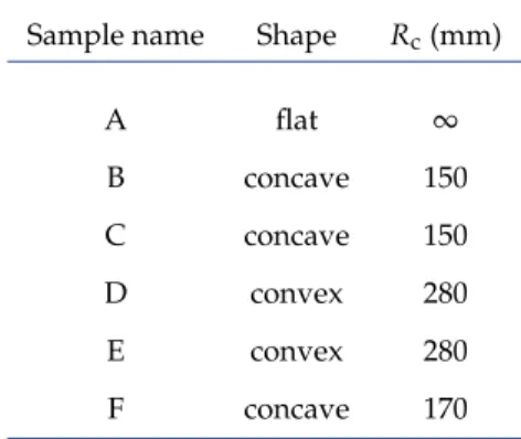
Table 1.List of CMOS samples tested in this paper, with their shape and radius of curvature (Rc).

Sample name Shape Rc(mm)

A flat ∞ B concave 150 C concave 150 D convex 280 E convex 280 F concave 170

3. CALIBRATION OF INTERNAL TEMPERATURE SEN-SOR

Some of the quantities that characterize a detector are highly de-pending on the temperature of the die itself (e.g. the dark cur-rent), thus a crucial step is to determine its temperature while the measurement is performed. CMV20000 detectors have in-ternal temperature sensors that can be used to monitor the chip temperature. Two registers – register 101 and 102 – are read-out from the chip by using the CMV20000 Evaluation Kit (Fig-ure2a). The values of these registers are related to the tempera-ture of the chip as follows:

T=l× (256×r102+r101) +q, (1)

where r102and r101are the register values. As l and q are

dif-ferent for each CMOS sensor, we must provide an independent temperature measurement of the die and relate that to the reg-ister values as in Equation1.

A. Internal temperature sensor calibration: methodology and set-up

We used a set of four thermocouples type K connected to a Quad MAX31856 board, that converts the output of the ther-mocouples in temperature values. We powered it and read it out with an Arduino MKR1000.

The thermocouples were glued to the back of four distinct copper blocks as in Figure2b. These blocks have dimensions of

Fig. 2.a: temperature calibration system installed inside the CMV20000 Evaluation Kit. The green/white cables are the thermocouples glued at the back of the copper blocks. b: schematic view from the back of the temperature calibration system where the thermocouples are glued. c: schematic view from the side of the temperature calibration system where the position of the CMOS and of the ceramic support is shown from the left.

8 mm×8 mm and a thickness of 3.2 mm. They sample the tem-perature at the back of the ceramic support of the CMV20000 chip in a region corresponding to its sensitive area (Figure2c). For the flat CMOS sensor this ceramic support is located imme-diately below the chip. The curved CMOS, however, addition-ally have the substrate used in the curving process (Section2), which is between the chip and the ceramic support. For the curved samples C, D, E and F this substrate is made of invar, that facilitates heat dissipation, for sample B (the first prototype made) it is made of plastic. A difference in the temperature cal-ibration of the samples is therefore expected.

Finally, a 3D-printed plastic structure holds the copper blocks together (Figure2). The thermal link between the back of the ceramic support and the copper blocks was enhanced by applying some thermal grease at the top of the blocks. By using this temperature calibration system – the four thermocouples with all the mechanical supports and the electronics – we have four different measurements of temperature from different ar-eas of the back side of the CMOS. In order to have an indepen-dent temperature probe of the front surface of the detectors, we also used an IR camera (FLIR I60BX, Figure3).

The internal temperature sensor of each detector was cali-brated singularly, by mounting the temperature calibration sys-tem at its back. After powering the detector on, we readout at

the same time: r102 and r101, the four thermocouples and we

acquired an image with the IR camera pointing at the front of the sensor. This image provides the temperature of the center of the CMOS sensor. We, then, let the sensor warm up (due to current flowing through it) and we repeated these steps again until it reached a stable temperature.

Fig. 3.Image from the IR camera (FLIR I60BX) used to sample the temperature of the front surface of the CMOS sensors.

B. Internal temperature sensor calibration: results

The temperature calibration system, provides a way to mea-sure the change in temperature between two different meamea-sure- measure-ments, but does not provide an estimate for the error on the absolute temperature value. To test the accuracy of the thermo-couples, we compared the temperature measured on average by the four thermocouples with the ones given by a mercury ther-mometer and a KIMO data logger (KISTOCK model KH210). We readout the temperature probes at a refrigerator tempera-ture (∼ 6o_{C) and we found that they all matched within the}

respective errors. By repeating the test at room temperature (∼27oC) the result did not change. We can, therefore, conclude that the absolute value of temperature provided by the thermo-couples is accurate within±0.5oC (the error here was the largest temperature mismatch found).

For each CMOS sensor described in this paper, we produced linear fits – as in Equation 1– by relating the values of regis-ter r102and r101to the temperature of the chip measured either

with the IR camera or with the thermocouples value, averaged over all four of them. For the flat sensor the presence of the pro-tective window in front of the chip prevented us from acquiring the IR camera images. In this case only the thermocouples mea-surements were performed.

The results of the fits are presented in Table2. The values of temperature obtained by substituting the IR camera parameters (lIRand qIR) are always larger than what we obtain by

substitut-ing the thermocouples parameters (lterand qter). The last two

columns of Table2show the parameters of the fit to the tem-perature measured by the thermocouple located at the center of the detector. Those values provide temperatures closer to the IR camera estimations, for most curved CMOS.

The difference between the value averaged over all four ther-mocouples and the value obtained by the central thermocouple can be explained by the presence of a gradient of temperature across the chip and its center being on average∼ 1oC hotter than the edges. As both the IR camera and the central thermo-couple sample the temperature at the center of the CMOS sen-sor, their agreement shows that the temperature calibration sys-tem provides an unbiased measurement. However we still find a non negligible discrepancy for sample B. Even when consid-ering its central thermocouple values, we have∼2oC constant offset between these and the IR camera measurements. This might be due to the presence of the plastic substrate between the CMOS chip and the ceramic support. Such substrate would prevent the dissipation of heat, generating in this way an offset in temperature.

As in this paper we are interested on characterizing the full sensitive surface of the detectors and not just its center, we used the temperature calibration results obtained from the average of all four thermocouples and kept the IR results as redundant test.

ter ter IR IR Cter Cter A 0.32±0.01 -357.3±13.5 – – 0.330±0.008 -371.4±10.6 B 0.32±0.01 -297.1±11.1 0.34±0.02 -311.6±16.6 0.342±0.008 -313.2±7.9 C 0.321±0.003 -293.9±3.4 0.33±0.01 -298.9±9.3 0.338±0.006 -310.1±5.9 D 0.295±0.004 -276.4±4.7 0.33±0.01 -314.5±13.1 0.311±0.002 -292.3±1.9 E 0.309±0.004 -292.7±3.9 0.307±0.003 -290.3±3.6 0.324±0.005 -308.2±4.7 F 0.333±0.006 -321.6±6.5 0.31±0.03 -300.2±28.2 0.345±0.006 -332.8±6.8

Once a reliable calibration for the internal temperature sensors was established, we used them as temperature monitor for each measurement performed during the CMOS sensors characteri-zation.

4. CHARACTERIZATION OF CMOS: TESTED QUANTI-TIES AND METHODOLOGY ADOPTED

The general aim of this paper is to characterize the CMOS sen-sors and evaluate the impact of the curving process on their per-formances. The measured characterization quantities include 6 main criteria [19,20]: gain of the detector, dark current, read-out noise (RON), pixel response non-uniformity (PRNU), dy-namic range (DR) and full well capacity (FW). These features are briefly described in the following Section.

A. Measured quantities for characterization

The dark current is due to the thermal agitation of the electrons within the semiconductor and it is extremely sensitive to the temperature of the detector itself. In Section3we established our own temperature calibration system which allowed us to calibrate the internal temperature sensor of the CMV20000 chip, used as temperature monitor during the characterization mea-surements.

The dark current is a source of "unwanted" signal that puts stringent limits to the performances of the detector and it has to be carefully characterized and subtracted to any image, to improve its quality. As the averaged number of counts on the detector grows linearly as a function of exposure time, the dark current is measured by reading out the detector at different ex-posure times in complete darkness conditions and a fit to these measurements is performed. By computing the mean signal of a dark frame, readout after 0 s of exposure time, we also obtain the bias level – a positive offset due to the constant voltage ap-plied by the electronic.

The readout noise (RON) is due to the scatter generated by the non perfectly reproducible conversion between analog to digital number, and the random fluctuation in the output sig-nal introduced by the readout electronic. The RON is obtained from the temporal noise, which in turn estimates the change of the output value of the pixels from contiguous exposures to a constant illumination level (valid also for dark frames). As the temporal noise, σtempis composed of the RON and of the shot

noise (due to the dark current or to the exposure to light) its value, when obtained from a set of dark frames at 0 s exposure time, is equivalent to the RON itself.

The gain of a detector determines how many charges col-lected in each pixel are assigned to a digital number in the im-age. The gain and the square of the temporal noise are in a linear relation as in the following Equation:

σ_temp2 =const+k(Smean−Soffset), (2)

where k is the gain in units of DN/e−and Smean−Soffsetare the

mean signal of the frame and the bias level (mentioned before) respectively. Here we assumed that the sensor is exposed to a uniform – across the detector surface – and stable illumination. For high illumination level (or longer exposure times), the PRNU starts becoming a dominant source of noise. The pix-els of a sensor have slightly different responses to incoming light and this effect generates the PRNU noise, which is di-rectly proportional to the number of electrons detected, Ne, as

in: Ne = fPRNUσPRNU. The proportionality factor is called

PRNU factor, fPRNU, and σPRNUis the PNRU noise.

In a frame, the total noise can be written as [20]:

σtot=

q

σ2

e+σRON2 +σPRNU2 (3)

where σeis the photon noise, σRON is the readout noise, and

σ_PRNUis the PRNU noise. It should be pointed out that Equa-tion3only deals with RON to first order [as indicated in19]. By considering that the PRNU noise has a spatial dependence but not a temporal one, the subtraction of two frames, obtained at the same exposure time and the same uniform level of illumina-tion, provides a new frame that contains only the RON and the photon noise. From this the σeis obtained and by substituting

it in Equation3, σPRNUand fPRNUare measured.

Finally the dynamic range – the capability of the detector to be sensitive at high and low signal levels at the same time – and the full well capacity – the amount of charges a pixel can hold before saturating – are defined as follows:

DR=20log(Smax/RON), FW=Smax−Soffset, (4)

where Smaxis the saturation limit, RON is the readout noise and

B. Data acquisition

A set of measurements was performed for each of the CMOS die listed in Section2. The exposure time used for these tests varied between 0.0002 s and the values at which saturation of the detector was reached, for exposures to uniform light – also called flat fields – and up to 0.96 s for exposures in complete darkness – or dark exposures.

The measurements were made by acquiring frames with shorter and longer exposure times in mixed order. The alter-nation of these reduces (if not eliminates altogether) the impact of systematic effects due to light level drifts or small temper-ature fluctuations (< _0.1o_{C). Thirty frames were acquired for}

each exposure time, with camera gain set to 1. For each of the 30-block frames, the values of the internal temperature sensor were readout (Section3).

The setup used for the flat field frames included an integrat-ing sphere, illuminated by a tungsten bulb located inside an-other smaller integrating sphere. The integrating sphere was placed at a distance of 1.0 m from the sensor to achieve a uni-form illumination of its surface. Care was taken to reduce the scattered light, by using light baffles along the path from the integrating sphere to the detector housing.

The measurements were performed at a room temperature of 21.0±1.0oC, where the error is considered over the acquisi-tion time for all the samples,∼ 5 days. The variation during the full testing of a single detector was±0.1oC. The temperature of the CMOS chips was monitored by the internal temperature sensor, calibrated as explained in Section3. Table3shows the temperature measured in average during the full characteriza-tion of a single detector and the errors in these estimates are the standard deviations from the average temperature measured. For sample A, C, E and F the temperature was∼35.0oC.

Table 3.Averaged temperature values for the different CMOS sensors, during the characterization measurements.

T (oC) A 34.9±0.2 B 33.1±0.2 C 35.2±0.2 D 40.1±0.5 E 35.1±0.1 F 34.9±0.1

Sample D was always at a higher temperature of 40.1±0.5oC. As we do not have a measurement of its temperature when the sensor was still flat, we do not know if this characteristic was introduced during the curving process. This different operating temperature might be due to intrinsic properties of the die. For sample B we have to consider that the measured temperature of 33.1±0.2oC (in Table3), corresponds to 35.1oC, as its plastic sub-strate creates a∼2oC bias between the real surface temperature and the measured one (see SectionB).

C. Methodology adopted for the characterization of curved CMOS

As specified in SectionBa set of 30 frames were acquired for each exposure time in the dark frames. From these, a median image was obtained and a mean dark signal level was estimated from the average over all pixels. The dark current and the bias level were, hence, obtained by fitting these estimates as func-tion of the exposure time.

The temporal noise, described in SectionA, was evaluated by building an image of the standard deviation of the 30 frames. If in the previous case we computed the median image, this time we estimated the standard deviation, among the the 30 frames, of each pixel in the image, creating a single image made of standard deviations. Then, we obtained the temporal noise for a specific exposure time, by averaging over the pixels of this standard deviation image. From this we obtained the RON as explained in SectionA.

We applied the same process to create the median image/mean signal level and the standard deviation im-age/temporal noise, also from the flat field frames. The mea-sured temporal noise and the mean signal level for several ex-posure time values were, thus, fitted according to the linear re-lation in Equation2, and the gain, k, was obtained.

The noise of an image contains also the PRNU, which does not depend on time. Thus,by subtracting two frames exposed to the same uniform light level for the same amount of time and measuring the noise of this resulting image, we obtained the PRNU noise and the PNRU factor, as detailed in SectionA. However by using only two frames we still have the influence of the temporal noise. We suppressed this effect by subtract-ing a randomly extracted frame to each of the other 29 frames acquired per exposure time and then we computed the noise,

σd. With the average of the 29 σd, scaled by a factor of 2, we

estimated the shot noise. This, thus, led to σPRNUand fPRNU,

which is usually expressed as a percentage of the mean signal (Equation3).

5. RESULTS

In this Section we show the results of the characterization of all the curved samples and we compare them to the ones from the flat sample. We use this comparison to statistically asses the impact of the curving process on the performances of the detectors.

A. Measured dark current and RON

On the left column of Figure4are shown the dark current mea-surements (as described in Section4) and the linear fits for all samples (each row in the Figure4is a different detector). For ex-posure times larger than 0.048 s the measured signal increases linearly, as the charges due to the dark current accumulate in the pixels. The black line in the plots are the linear fits to the data, from which the dark current value in DN/s (the slope of the fit) and the bias level (the intercept of the fit) are obtained.

After applying the gain to each detector (see Section B), we find the dark current values in Table4. As already men-tioned these measurements were performed at a temperature of∼ 35oC for all samples (except for sample D) and the dark current values for the curved detector samples are consistently smaller than the one of the flat detector. More specifically they differ of: sample B 28%, sample C 32%, sample E 39% and sam-ple F 38%. The higher temperature of samsam-ple D makes the com-parison of its dark current with the dark current of the other

the responses are not linear. This feature is found in all sensors, thus, we concluded that it is an intrinsic characteristic of the CMV20000 CMOS. This also implies that the measured value of the bias level is higher than the value from the fit of the dark current. We used this higher value for the bias level in the rest of the paper (it is also the one written in Table4), as we followed the definition of bias: the mean value of the median frame with the shortest exposure time acquired in darkness.

From the median image of the dark exposure with the short-est exposure time, we additionally evaluated the column tem-poral noise, by computing the standard deviation from the mean value of each column in the image. These results are plot-ted vs column number in the middle column of Figure4. The column temporal noise of the curved samples does not present any large variation with respect to the flat sample case, and it shows the same behavior with increasing noise values towards the center and decreasing values at the edges. The measure-ments of the curved sensors also present mostly smaller values with larger scatter, compared to the flat sensor values.

The column temporal noise of the C sample shows signif-icantly larger scatter due to the presence of one or more hot pixels per column. The surface of this sample is slightly de-formed, especially around the center. The deviation from a per-fect sphere is visible from Figure1. This, however, does not imply that the surface deformation has an impact on the noise of the detector, as the dark current did not show any sign of difference with respect to the other samples. As the quality of the wafer of this specific chip was graded lower with respect to the other detectors presented here, those hot pixels could have been present even before the thinning and curving process. We can not draw conclusive reason for this peculiar behavior, since the properties of the sensors, before the curving process, are un-known.

The RON was estimated from the temporal noise of the dark exposures acquired at the shortest exposure time, as explained in Section4. These values are shown in Table4.

B. Measured gain, dynamic range and full well capacity

The gain was measured as explained in Section4, from a set of flat fields where the sensors are exposed to uniform and stable illumination. The average signal measured on the frames grows linearly for exposure times larger than 0.048 s until it reaches the saturation limit of 4095 DN (set by the Analog Digital Con-verter, 12-bit per pixel) and plateaus. The saturation limit is specified in Table4for all the detectors tested. All of them reach it at 4095 DN except for sample C that saturates at 3951 DN. By using the measured saturation limit, RON and bias level, we obtained the values (in Table4) of dynamic range and full well capacity as in Equation4.

The right column of Figure4shows the squared values of the temporal noise of the detectors against the mean signal sub-tracted by the bias level [19]. The linear trend due to the accu-mulation of the charges inside the pixels (described by Equa-tion 2), appears for values of mean signal - offset between 1000 DN and 3000 DN. The black lines in the plots on the right column of Figure4are the fits to the data from which we obtain

variation found among the gain values is considered within the manufacturing scatter and therefore not pointing to any specific effect due to the curving process.

The last characteristic quantity shown in Table4is the PRNU factor, fPRNU, computed as explained in SectionC. The PRNU

factor values do not present large differences among the sam-ples, flat and curved.

6. CONCLUSIONS

The recent progress made towards the manufacturing of curved detectors represents a step forward to the creation of more com-pact and performing optical systems with very wide applica-tions. It also opens the possibility to new designs, whose re-alization was technologically impossible before. Here, we pre-sented the characterization results of a sample of five curved CMOS detectors developed within a collaboration between CEA-LETI and CNRS-LAM. These detectors are CMV20000 with 20 Mpix (manufactured by CMOSIS) and they have been curved with different shapes and radii of curvature over the full sensitive area of 24x32 mm2. The curved detector sample is composed of two concave curved down to Rc =150 mm,

another concave with Rc =170 mm and two convex with

Rc=280 mm.

Since the packaging of the detectors is the same as the origi-nal one, it is possible to plug the detectors in directly in any in-terface or camera that was already built for the flat off-the-shelf sensor. In order to perform the tests and readout the detectors, we used the CMV20000 Evaluation Kit (from CMOSIS). This also allowed us to readout the internal temperature sensors of the CMV20000 chips.

These temperature sensors were calibrated against four ther-mocouples for all the detectors tested in this paper (Section3). The thermocouples were glued at the back of small copper blocks, that were in turn thermally linked to the back of the ceramic support located below the detector sensitive area. Such thermocouples have been readout at the same time of the inter-nal temperature sensor. The measured temperature was sam-pled from room temperature (∼19o_{C) until full thermalization}

of the sensors (∼ 35−40oC). Once the calibration of the inter-nal temperature sensors was achieved, the thermocouples were removed.

In Section4we described the quantities to characterize, the setup used, and the methodology for performing the measure-ment and analyzing the results. The same characterization steps were repeated for all the sensors in the test sample. From Table4we have an overview of the results and we find them to be mostly homogeneous between the flat and curved samples. A large difference (with respect to the other detectors) in dark current is measured for sample D (one of the convex shaped). For this sample the dark current is almost 3 times larger than the dark current measured for the others, and this is due to the larger temperature that the sensor reached while performing its characterization. While all the other samples reached a stable characterization temperature of∼35.0oC, sample D was tested at∼40.0oC.

Fig. 4.Left column: the blue solid circles are the median values of the dark exposure frames as function of exposure time, the black solid lines are the fits to the data. Middle column: column temporal noise vs column number of the sensor. The vertical black line indicates the column in the middle of the frame. Right column: squared temporal noise of flat field frames as function of mean signal-offset (bias level). The black lines are the fits to the data for mean signal-offset between 1000 DN and 3000 DN. Each row of the Figure represents the measured quantities for a single detector (specified on the left side of the Figure).

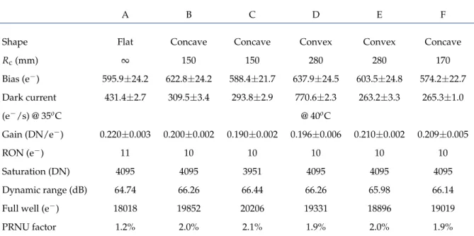
Table 4.Values for the electro-optical characterization of the flat and curved CMV20000 CMOS sensors. Note that the same method-ology has been applied to all sensors and that sample D was measured at a different temperature with respect to the others.

A B C D E F

Shape Flat Concave Concave Convex Convex Concave

Rc(mm) ∞ 150 150 280 280 170 Bias (e−_{) 595.9±24.2 622.8±24.2 588.4±21.7 637.9±24.5 603.5±24.8 574.2±22.7} Dark current 431.4±2.7 309.5±3.4 293.8±2.9 770.6±2.3 263.2±3.3 265.3±1.0 (e−/s) @ 35oC @ 40oC Gain (DN/e−) 0.220±0.003 0.200±0.002 0.190±0.002 0.196±0.006 0.210±0.002 0.209±0.005 RON (e−) 11 10 10 10 10 10 Saturation (DN) 4095 4095 3951 4095 4095 4095 Dynamic range (dB) 64.74 66.26 66.44 66.26 65.98 66.14 Full well (e−_{) 18018 19852 20206 19331 18896 19019} PRNU factor 1.2% 2.0% 2.1% 1.9% 2.0% 1.9%

When we compared the dark current value for the flat sensor, to the dark current measured for the other samples (excluding sample D), we obtained substantially lower values for the latter ones: from 28%, up to a maximum of 39% difference. A similar decrease of dark current in curved CMOS sensors was already found in other works [5,9] and has been attributed to an alter-ation of the band gap in the sensitive area of the devices due to the strain induced in the curving process. As in our case the curving process is made without fixing the edges (as in [5]) and the dimension of the sensors is much larger than their thick-nesses, some decrease in dark current is expected in our spheri-cally curved samples [10]. However it is not excluded that some amount of this difference might be due to intrinsic properties of the samples themselves. This could also explain their similar dark current values.

We also measured a smaller readout noise of 10 e−_{for all the}

curved sensors with respect to the 11 e−for the flat sensor. This smaller RON generates a larger dynamic range>_{66 dB, against}

the 64.74 dB of the flat sensor. We find no significant difference in the bias level, as the values mostly match within the errors. We also find similar behavior of the column temporal noise be-tween all sensors, where the curved samples presented smaller values, with larger scatter, compared to the flat one. From the measurements, the gains show a discrepancy from 5% to 16% between the curved sensors compared to the flat one, which might be due to an intrinsic characteristic that the chips already had before curving them.

The PRNU factors of the curved samples show an increase

of∼0.8% with respect to the value for the flat sensor. The dif-ference between these is not significant. This also holds true for sample C, that even having a deformed shape, does not present any particular degradation in its performances.

From the overall performances tested in this paper, we con-clude that the curving process shown here does not impact the main electrical characteristics of the detectors and in some cases, e.g. the dark current, it might even improve them. The astro-nomical community can particularly gain from this characteris-tic.

The next step for this work is to verify the quality of the de-tector surface, and if necessary, improve the curving technique until it reaches the required precision for astronomical applica-tions. Once this is achieved, a new prototyping phase can begin to develop curved CCDs.

Funding Information. ERC (European Research Council) (H2020-ERC-STG-2015-678777 ICARUS program), the French Research Agency (ANR) through the LabEx FOCUS ANR-11-LABX-0013. Acknowledgments. The authors acknowledge the support of the European Research council through the H2020-ERC-STG-2015-678777 ICARUS program.

REFERENCES

1. G. H. Sanders, “The Thirty Meter Telescope (TMT): An International Observatory,” J. Astrophys. Astron.34, 81–86 (2013).

2. M. Johns, C. Hull, G. Muller, B. Irarrazaval, A. Bouchez, T. Chylek, C. Smith, A. Wadhavkar, B. Bigelow, S. Gunnels, B. McLeod, and

4. C. Atkins, C. Feldman, D. Brooks, S. Watson, W. Cochrane, M. Roulet, P. Doel, R. Willingale, and E. Hugot, “Additive manufactured x-ray op-tics for astronomy,” in Society of Photo-Optical Instrumentation

En-gineers (SPIE) Conference Series, , vol. 10399 of Society of Photo-Optical Instrumentation Engineers (SPIE) Conference Series (2017),

p. 103991G.

5. B. Guenter, N. Joshi, R. Stoakley, A. Keefe, K. Geary, R. Free-man, J. Hundley, P. Patterson, D. Hammon, G. Herrera, E. SherFree-man, A. Nowak, R. Schubert, P. Brewer, L. Yang, R. Mott, and G. McKnight, “Highly curved image sensors: a practical approach for improved opti-cal performance,” Opt. Express25, 13010 (2017).

6. O. Iwert, D. Ouellette, M. Lesser, and B. Delabre, “First results from a novel curving process for large area scientific imagers,” in High Energy,

Optical, and Infrared Detectors for Astronomy V, , vol. 8453 of Proc. SPIE (2012), p. 84531W.

7. D. Dumas, M. Fendler, N. Baier, J. Primot, and E. le Coarer, “Curved focal plane detector array for wide field cameras,” Appl. Opt.51, 5419 (2012).

8. K. Tekaya, M. Fendler, K. Inal, E. Massoni, and H. Ribot, “Mechani-cal behavior of flexible silicon devices curved in spheri“Mechani-cal configura-tions,” in 14th International Conference on Thermal, Mechanical and

Multi-Physics Simulation and Experiments in Microelectronics and Mi-crosystems, (IEEE - Institute of Electrical and Electronics Engineers,

Wroclaw, Poland, 2013), pp. 7 pages – Article number 6529978. 9. K. Itonaga, T. Arimura, K. Matsumoto, G. Kondo, K. Terahata, S.

Maki-moto, M. Baba, Y. Honda, S. Bori, T. Kai, K. Kasahara, M. Nagano, M. Kimura, Y. Kinoshita, E. Kishida, T. Baba, S. Baba, Y. Nomura, N. Tanabe, N. Kimizuka, Y. Matoba, T. Takachi, E. Takagi, T. Haruta, N. Ikebe, K. Matsuda, T. Niimi, T. Ezaki, and T. Hirayama, “A novel curved cmos image sensor integrated with imaging system,” in 2014

Symposium on VLSI Technology (VLSI-Technology): Digest of Tech-nical Papers, (2014), pp. 1–2.

10. J. A. Gregory, A. M. Smith, E. C. Pearce, R. L. Lambour, R. Y. Shah, H. R. Clark, K. Warner, R. M. Osgood, D. F. Woods, A. E. DeCew, S. E. Forman, L. Mendenhall, C. M. DeFranzo, V. S. Dolat, and A. H. Loomis, “Development and application of spherically curved charge-coupled device imagers,” Appl. Opt.54, 3072 (2015).

11. P. Swain and D. Mark, “Curved CCD detector devices and ar-rays for multispectral astrophysical applications and terrestrial stereo panoramic cameras,” in Optical and Infrared Detectors for Astronomy, , vol. 5499 of Proc. SPIE J. D. Garnett and J. W. Beletic, eds. (2004), pp. 281–301.

12. K. Tekaya, M. Fendler, D. Dumas, K. Inal, E. Massoni, Y. Gaeremynck, G. Druart, and D. Henry, “Hemispherical curved monolithic cooled and uncooled infrared focal plane arrays for compact cameras,” in Infrared

Technology and Applications XL, , vol. 9070 of Proc. SPIE (2014), p.

90702T.

13. W. J. Borucki, D. Koch, G. Basri, N. Batalha, T. Brown, D. Caldwell, J. Caldwell, J. Christensen-Dalsgaard, W. D. Cochran, E. DeVore, E. W. Dunham, A. K. Dupree, T. N. Gautier, J. C. Geary, R. Gilliland, A. Gould, S. B. Howell, J. M. Jenkins, Y. Kondo, D. W. Latham, G. W. Marcy, S. Meibom, H. Kjeldsen, J. J. Lissauer, D. G. Monet, D. Morrison, D. Sasselov, J. Tarter, A. Boss, D. Brownlee, T. Owen, D. Buzasi, D. Charbonneau, L. Doyle, J. Fortney, E. B. Ford, M. J. Hol-man, S. Seager, J. H. Steffen, W. F. Welsh, J. Rowe, H. Anderson, L. Buchhave, D. Ciardi, L. Walkowicz, W. Sherry, E. Horch, H. Isaac-son, M. E. Everett, D. Fischer, G. Torres, J. A. JohnIsaac-son, M. Endl, P. MacQueen, S. T. Bryson, J. Dotson, M. Haas, J. Kolodziejczak, J. Van Cleve, H. Chandrasekaran, J. D. Twicken, E. V. Quintana, B. D. Clarke, C. Allen, J. Li, H. Wu, P. Tenenbaum, E. Verner, F. Bruhweiler, J. Barnes, and A. Prsa, “Kepler Planet-Detection Mission: Introduction and First Results,” Science.327, 977 (2010).

A. Gil de Paz, J. H. Knapen, and J. C. Lee, eds. (2017), pp. 199–201. 16. E. Muslimov, D. Valls-Gabaud, G. Lemaître, E. Hugot, W. Jahn, S. Lombardo, X. Wang, P. Vola, and M. Ferrari, “A fast, wide-field and distortion-free telescope with curved detectors for surveys at ultra-low surface brightness,” ArXiv e-prints (2017).

17. A. Kelz, S. Kamann, T. Urrutia, P. Weilbacher, and R. Bacon, “Multi-Object Spectroscopy with MUSE,” in Multi-“Multi-Object Spectroscopy in the

Next Decade: Big Questions, Large Surveys, and Wide Fields, , vol.

507 of Astronomical Society of the Pacific Conference Series I. Skillen, M. Balcells, and S. Trager, eds. (2016), p. 323.

18. B. Chambion, C. Gaschet, T. Behaghel, A. Vandeneynde, S. Caplet, S. Gétin, D. Henry, E. Hugot, W. Jahn, S. Lombardo, and M. Fer-rari, “Curved sensors for compact high-resolution wide-field designs: prototype demonstration and optical characterization,” in Society of

Photo-Optical Instrumentation Engineers (SPIE) Conference Series,

, vol. 10539 of Society of Photo-Optical Instrumentation Engineers

(SPIE) Conference Series (2018), p. 1053913.

19. J. R. Janesick, Photon Transfer DN toλ (SPIE, 2007).