Geometric Feature Extraction by a Multi-Marked Point Process

HAL Id: inria-00503140

https://hal.inria.fr/inria-00503140

Submitted on 28 Jan 2013

HAL is a multi-disciplinary open access

archive for the deposit and dissemination of

sci-entific research documents, whether they are

pub-lished or not. The documents may come from

teaching and research institutions in France or

abroad, or from public or private research centers.

L’archive ouverte pluridisciplinaire HAL, est

destinée au dépôt et à la diffusion de documents

scientifiques de niveau recherche, publiés ou non,

émanant des établissements d’enseignement et de

recherche français ou étrangers, des laboratoires

publics ou privés.

Process

Florent Lafarge, Georgy Gimel’Farb, Xavier Descombes

To cite this version:

Florent Lafarge, Georgy Gimel’Farb, Xavier Descombes. Geometric Feature Extraction by a

Multi-Marked Point Process. IEEE Transactions on Pattern Analysis and Machine Intelligence, Institute of

Electrical and Electronics Engineers, 2010, 32 (9), �10.1109/TPAMI.2009.152�. �inria-00503140�

Geometric Feature Extraction by a Multi-Marked

Point Process

Florent Lafarge, Georgy Gimel’farb and Xavier Descombes

Abstract—This paper presents a new stochastic marked point process for describing images in terms of a finite library of geometric objects. Image analysis based on conventional marked point processes has already produced convincing results but at the expense of easy parameter tuning, short computing time, and unspecific models. Our more general multi-marked point process has simpler parametric setting, yields notably shorter computing times and can be applied to a variety of applications. Both linear and areal primitives extracted from a library of geometric objects are matched to a given image using a probabilistic Gibbs model, and a Jump-Diffusion process is performed to search for the optimal object configuration. Experiments with remotely sensed images and natural textures show the proposed approach has good potential. We conclude with a discussion about the insertion of more complex object interactions in the model by studying the compromise between model complexity and efficiency.

Index Terms—Object extraction, remote sensing, texture analysis, Stochastic models, Monte Carlo simulations.

✦

1

I

Probabilistic methods are now widespread in image analysis. They have proved to be powerful tools to solve inverse optical problems such as image segmentation or image restoration [1], [2]. Since the mid-nineties, many works have extended the initial pixel based approaches to the concept of object in order to deal with feature recognition problems. In particular, stochastic models have shown good potentialities in extracting rectilinear shapes. Generally, configurations of geometric objects are sampled from probability distributions defined in config-uration space, Markov Chain Monte Carlo (MCMC) [3], [4] being one of the most popular families of samplers. In various application domains, from 3D reconstruction [5], [6] to texture modeling [7], [8], [9], the MCMC samplers are efficient for object extraction in large configuration spaces from any type of probability distributions. Stochastic models based on marked point processes are among the most efficient approaches and have al-ready led to convincing experimental results in vari-ous image analysis applications such as extraction of buildings [11], road markings [13], vascular trees [14], road networks [12], tree crowns [10] or populations of birds [15]. The marked point processes, detailed in [16], exploit random variables whose realizations are con-figurations of geometrical objects, e.g. rectangles [11],

• F. Lafarge and Georgy Gimel’farb are with the Department of Computer

Science, University of Auckland, Private Bag 92019, Auckland 1142, New Zealand. E-mail: flafarge(at)gmail.com, g.gimelfarb(at)auckland.ac.nz

• _{X. Descombes is with the Ariana Research Group, INRIA Sophia}

An-tipolis, 2004 route des Lucioles 06902 Sophia AnAn-tipolis, France. E-mail: Xavier.Descombes(at)inria.fr

Manuscript received October 19, 2008; revised April 8, 2009; accepted June 3, 2009.

Recommended for acceptance by S.-C. Zhu.

For information on obtaining reprints of this article, please send e-mail to: [email protected], and reference IEEECS Log Number TPAMI-xxxxxxx. Digital Object Identifier no. 1xxxxxxxxxxxxx.

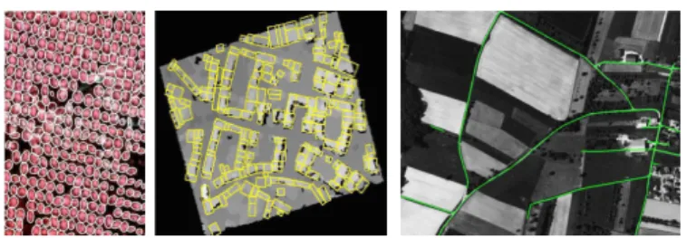
Fig. 1. Results of marked point process based models c

°INRIA. Extraction of (from left to right) tree crowns [10], building footprints [11], and road networks [12].

[13], segments [12], [14], or ellipses [10], [15]. After a probability distribution measuring the quality of each object configuration is specified, the maximum density estimator is searched for by an MCMC technique based on the birth-and-death sampler [17] coupled with the conventional simulated annealing [18]. Such processes allow the description of complex spatial interactions between the objects. As exemplified in Figure 1, image representations produced by these stochastic models are particularly suitable for solving object recognition prob-lems. However, these models have the following three drawbacks:

• Lack of generality: Each model is associated with only

a specific application (in all the above mentioned works, a marked point process is limited to a sin-gle type of objects with simple geometric shape). Moreover, the complexity of interactions between the objects defined in the model makes it impos-sible to generalize each particular model to another application.

• Lengthy computational time: Although proposition

kernels are developed to speed up the process, the birth-and-death sampler remains very slow, espe-cially at low temperatures. For example, the result

presented in Figure 1-center has been obtained in more than three hours on a 3 GHz processor.

• Trial-and-error parameter tuning: Many parameters

(up to ten in most cases) are to be used to define the interactions. They are tuned by trial and error since parameter estimation techniques do not efficiently work with such large configuration spaces. This procedure is long and complex since a Monte Carlo simulation has to be used at each iteration of the tuning.

This paper proposes a new generalized marked point process called by extension a multi-marked point process. It provides results that approach by accuracy those obtained with models based on the conventional marked point processes [10], [11], [12], [13], [14], [15], but pro-duces these results in a shorter time and can be applied to a large range of applications without changing the un-derlying model. Our proposal modifies the conventional marked point processes as follows:

• Joint sampling of multiple objects: The process must

jointly sample different types of geometric objects (e.g. linear and areal objects such as segments and polygons) in order to extend the level of generality.

• Constrained object interactions: The interactions

be-tween the objects must be simplified and reduced to only the essential ones in order to (i) significantly decrease the number of tuning parameters, (ii) ex-tend the level of generality by avoiding specific interactions, and (iii) use gradient descent based sampling.

• Introducing diffusion dynamics: Diffusion dynamics

would allow a significant acceleration of the con-vergence. The conventional marked point process based models cannot use such a dynamics because the complexity of their probability distributions (usually gradients of their Gibbs energy (see section 2.2) do not satisfy the Lipschitz continuity condi-tion [19]). The Jump-Diffusion processes introduced by Grenander et al. [20] represent a class of ran-dom samplers which efficiently combine both Monte Carlo techniques and diffusion dynamics.

This paper extends the work we presented in [21] by detailing both the multi-marked point process model and the optimization technique, as well as presenting new results and comments on various remote sensing applications and texture descriptions. The paper is orga-nized as follows. Section 2 overviews the marked point processes and proposes their extension to the multi-marked ones that deal with the different object types. Section 3 introduces a Gibbs energy model adapted to different types of geometric objects specified by a chosen mark library. The model is sampled by a Jump-Diffusion process detailed in Section 4. Experimental results for remote sensing and texture description problems are given in Section 5. Section 6 proposes a discussion about the insertion of more complex object interactions in the model by studying the compromise between model

complexity and efficiency. Basic conclusions are outlined in Section 7.

2

P

The marked point processes have been introduced in image processing by Baddeley and Van Lieshout [22], and developed and extended further in [16], [23], [24]. These stochastic models can be considered as an exten-sion of conventional Markov random fields [25] such that random variables are associated not with pixel values but with geometrical shapes describing the image. An overview of marked point processes is provided below.

2.1 Point processes

Let X be a point process living in a continuous bounded set K = [0, Xmax]×[0, Ymax] supporting an image. X is a

measurable mapping from an abstract probability space (Ω, A, P) to the set of configurations of points of K:

∀ω ∈ Ω, xi∈ K, X(ω) = {x1, ..., xn(ω)} (1)

where n(ω) represents the number of points associated with the event ω. The homogeneous Poisson process is the reference point process. Let ν(.) be a positive measure on K. A Poisson process X with intensity ν(.) verifies the two following properties:

• For every Borel set B ∈ K, the random variable

NX(B) defining the number of points of X in the

Borel set B follows a discrete Poisson distribu-tion with the mean ν(B), i.e. P (NX(B) = n) =

ν(B)n

n! e −ν(B)_.

• For every finite sequence of non intersecting

Borelian sets B1, ..., Bl, the random variables

NX(B1), ..., NX(Bl) are independent.

The Poisson process induces a complete spatial random-ness, given by the fact that the positions are uniformly and independently distributed. Its role is analogous to Lebesgue measures on Rd_.

2.2 Density and Gibbs energy

Complex point processes introducing both consistent measurements with data and interactions between points can be defined by specifying a density with respect to the distribution of a reference Poisson process. Let us consider an homogeneous Poisson process with intensity measure ν(.), and let h(.) be a non-negative function on the configuration space C. Then, the measure µ(.) having a density h(.) with respect to ν(.) is defined by:

∀B ∈ B(C), µ(B) = Z

B

h(x)ν(dx) (2)

A point process can be specified through a Gibbs energy U(x). The density h(x) of a configuration x is formulated using the Gibbs equation:

h(x) = exp −U (x)

where Z is a normalizing constant: Z =R_x∈Cexp −U (x). Generally, a Monte Carlo Markov Chain (MCMC) sam-pler coupled with a simulated annealing is used to find the maximum density estimator bx = arg max h(.) (this estimator also corresponds to the configuration minimiz-ing the Gibbs energy U (.), i.e. bx = arg min U (.) ). This optimization technique is particularly interesting since the density h(.) does not need to be normalized, and the complex computation of the normalizing constant Z is then avoided.

2.3 Marked and Multi-marked point processes

In order to model images in terms of geometrical fea-tures, it is possible to extend a point process by adding specific marks that associate a parametric object to each point. In many cases, the point corresponds to the center of mass of the object. A marked point process in S = K ×M is a point process in K where each point is associated with a mark from a bounded set M , for example, a set of radius values in case of disks.

The conventional marked point processes [10], [11], [12], [13], [14], [15] suffer from a lack of generality: they are limited to a single type of objects since the dimension of the mark space M is fixed (e.g. rectangles [11], [13], segments [12], [14], or ellipses [10], [15]). Ortner et al. [26] proposed to overcome this drawback by consider-ing two marked point processes each usconsider-ing a different type of objects (rectangles and segments). The two pro-cesses are sampled jointly by a Markov Chain Monte Carlo algorithm. However, in this approach, both energy formulations and simulated annealing tunings become too complex to manage since cooperative interactions between both processes must be taken into account. This model cannot be adapted in practice to deal with a large number of object types.

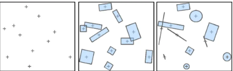
Fig. 2. Realizations of (from left to right) a point process, a marked point process of rectangles, and a multi-marked point process of rectangles/segments/circles.

We propose to generalize the conventional marked point process framework in order to jointly sample various types of geometric objects. To do so, we consider a finite library of marks allowing the definition of linear and areal features. The mark space M associated with this library is then specified as a finite union of mark bounded subsets Mq: M = Ns [ q=1 Mq (4)

where each subset Mq corresponds to one of the Ns

specific shape types. In other words, the associated marked point process is able to deal with objects having different numbers of control parameters. Such a process, that we can call by extension a multi-marked point process, implies significant changes with respect to the conven-tional approach such as restrictions on the data term (e.g. the measurement must be independent of the object type), the setting up of general interactions between the various object types, or the introduction of new propositional functions to switch the object type during the sampling.

3

P

G

The library of marks allows the representation of seven simple geometric patterns shown in Figure 3. Segments, lines, and line ends are specific to linear structures whereas rectangles, bands, band ends, and circles corre-spond to areal descriptors. All the objects have between three and five control parameters, including positional coordinates (cx, cy) of the object’s center that are

speci-fied by the point process in K. The other parameters, detailed in Table 1, represent the marks of the object types (e.g. the radius for circles; the length, width, and orientation for bands and rectangles). The parameters are defined in continuous domains, except for the object orientation defined in a discrete domain. The chosen set includes all basic objects used in the conventional marked point process based models. Thus, it is sufficient to produce detailed representations of a large range of scenes in terms of their linear and areal components.

Fig. 3. The library of marks.

TABLE 1

Parameter definition of the marks:s-the length;θ-the orientation angle;r-the radius;L, l-the height and width

respectively.

object type marks definition domains segment s, θ [smin, smax] × [0, π]

line s, θ [smin, smax] × [0, π]

line end s, θ [smin, smax] × [0, 2π]

circle r [rmin, rmax]

rectangle L, l, θ [Lmin, Lmax] × [lmin, lmax] × [0, π]

band L, l, θ [Lmin, Lmax] × [lmin, lmax] × [0, π]

band end L, l, θ [Lmin, Lmax] × [lmin, lmax] × [0, 2π]

3.2 Gibbs energy

Because the number of objects in any particular scene is unknown, and the objects have different numbers of

parameters, the configuration space C of our problem is defined as an union of subspaces Ck, each subspace

containing fixed numbers of objects of each type. A probability distribution P on the configuration space C is defined as a mixture of Pkdistributions on the subspaces

C_{k. We assume that unnormalized distributions Pkon Ck} have Gibbs densities of the form e−Uk(x) _{where U}

k is a

Gibbs energy associated with the configuration subspace C_{k (see Section 2.2).}

The energy Uk(x) takes into account both the consistency

Dk(x) between the objects and the image data and the

regularization constraint Rk(x) for the positioning of the

objects with no overlaps:

Uk(x) = Dk(x) + Rk(x); x∈ Ck (5)

3.2.1 The data coherence term

Dk(x) accumulates the local energy associated with each

object xi of the configuration x:

Dk(x) =

X

i

d(xi) (6)

where d(xi) is a measure of coherence of the object xi

with respect to the data (i.e. an image). This measure d(.) must satisfy two important conditions:

• Independence of the object type: In particular, the

object area must be taken into account in order to not favor linear or areal object types.

• Selection of ”attractive” objects: i.e. the well-fitted

objects must have a negative local energy (this feature is very important in the models using birth-and-death processes since it partly defines the object density in the scene).

In addition, d(.) must be differentiable and quickly computable in order to use diffusion dynamics during the optimization. We propose a function that is derived from the Mahalanobis distance and includes a threshold θattr > 0 that makes some objects attractive if the

function is negative: d(xi) =

( q

σ2 in+σout2 +ǫ

S(min−mout)2 − θattr if min6= mout

∞ otherwise (7)

Here, (min, σin) and (mout, σout) represent the mean pixel

intensities and standard deviations inside and outside the object, respectively (i.e. the blue and red areas on Figure 4). The width of the outside domain is fixed to 2 pixels in practice. S is the whole inside and outside area, and ǫ > 0 is an infinitesimal value allowing d(.) to be differentiable. The threshold θattr, being the only

parameter of the model, allows to select the attractive objects and tune the sensitiveness of the data fitting. This measure of coherence is based on signal homogeneity criteria inside and outside the object (See Figure 4). It could be improved by taking into account specific information such as contour accuracy or noise modeling. Nonetheless, this measure produces good experimental results as we can see on Figure 5, and the introduction

Fig. 4. Coherence measure between the object and the image data.

of additional criteria would strongly increase the com-puting time.

In addition, two variants of this measure are proposed in order to introduce radiometric information on target objects. By taking min> mout (respectively min< mout)

instead of min 6= mout in the definition domain of d(.)

(see Eq. 7), we can modify the measure in order to favor bright (respectively dark) objects with respect to the background. This variant of d(.) will be called dbright(.)

(respectively ddark(.)) and used for various experiments

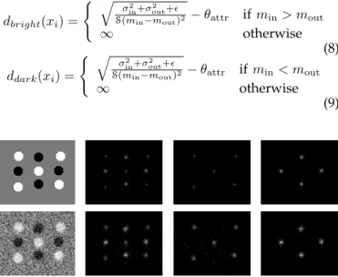
in order to obtain a more specific extraction of target objects. Figure 5 shows two sets of signal responses with disks from the d, dbright and ddark measures. The first

set corresponds to an ideal signal simulation. The black disk responses are slightly stronger than the white ones since the uniform bright grey background is closer to the white color than the black one. The second set shows the robustness of these measures with respect to noise and blur.

dbright(xi) =

( q _σ2 in+σout2 +ǫ

S(min−mout)2 − θattr if min> mout

∞ otherwise (8) ddark(xi) = ( q σ2 in+σout2 +ǫ

S(min−mout)2 − θattr if min< mout

∞ otherwise

(9)

Fig. 5. Responses of (from left to right)d,dbrightandddark

measures for a disk object on (top) exact and (bottom) noise and blur corrupted simulations.

3.2.2 The regularization constraint

Rk(x) introduces prior knowledge on the object layouts

by taking into account pairwise interactions between the objects. The conventional marked point processes use strong structural information by defining complex and

specific interactions such as inter-connections or mutual alignments of the objects [11], [12], [13], [14]. These com-plex interactions result in the above-mentioned critical problems (Section 1), such as trial-and-error tuning of many parameters. More generally, the introduction of such structural information in stochastic models requires special learning techniques such as the linear junction model presented in [27] or advanced thresholding meth-ods such as a contrario approaches [28].

To avoid these problems, we limit the interactions to the essential ones for developing a general model of the non-overlapping objects. Strong structural information can then be introduced in a subsequent analysis by develop-ing post-processdevelop-ing in order to connect the objects found. This term is expressed as follows:

Rk(x) =

X

xi,xj∈x

(eκg(xi,xj)_{− 1) (10)}

where g(xi, xj) taking values in [0, 1] quantifies the

rela-tive mutual overlap between the objects xi and xj, and

κ is a big positive real value (κ = 100) which strongly penalizes large overlaps. Under small overlaps between two objects, this prior will weakly penalize the global energy. But if the overlapping is high, this prior will act as a hardcore (i.e. a hard constraint: the prior energy takes a very high value), and the configuration will be practically banned.

4

O

J

-D

The search for an optimal configuration of objects is performed using the Jump-Diffusion process introduced by Grenander et al. [20], and used successfully in var-ious applications such as target tracking [29], [30] and image segmentation [31]. This process combines the conventional Markov Chain Monte Carlo (MCMC) al-gorithms [4] and the Langevin equations [19]. Both dynamics play different roles in the Jump-Diffusion process: the former performs reversible jumps between the different subspaces Ck, whereas the latter conducts

stochastic diffusion within each continuous subspace. The global process is controlled by a relaxation tem-perature T depending on time t and approaching zero as t tends to infinity. The estimation of the simulated annealing parameters are detailed in Section 4.3. The diffusions are interrupted by jumps following a discrete time step ∆t (in our experiments, ∆t = 50). At the very low temperature, the diffusion process plays a more important role: the time step is increased (∆t = 100) to speed up the convergence.

4.1 Jump dynamic

Reversible jumps between the different subspaces are performed according to families of moves called propo-sition kernels and denoted by Qm where m represents

the family of moves. The jump process performs a move from an object configuration x ∈ Ck to y ∈ Ck′ according

to a density Qm(x → y). Then the move is accepted with

the following probability: min µ 1,Qm(y → x) Qm(x → y) e−(Uk′(y)−Uk(x))_T ¶ (11) We use two different families of moves in order to jump between the subspaces.

• Birth-and-death kernel Q_BD allows for adding or

re-moving an object from a current object configura-tion. These transformations corresponding to jumps into the spaces of higher (birth) and lower (death) dimension are theoretically sufficient to visit the whole configuration space [16], [17]. In practice, we choose to add or remove an object following a Poisson distribution. If an object is added, its type is randomly chosen and its parameters are chosen according to uniform distributions over the parameter domains.

• Switching kernel Q_S allows us to switch the type

of an object (e.g. a circle by a rectangle). Contrary to the previous kernel, this move does not change the number of objects in the configuration. How-ever, the number of parameters can be different (e.g. three parameters for a circle are substituted by five parameters for a rectangle). This kernel creates bijections between the different types of objects [4]. The computation of both the kernels is detailed in Ap-pendix. Usually the jump processes [6], [10], [11], [12], [13], [14], [15] use a perturbation kernel that allows the exploration of each subspace by modifying only parameters of the objects. In our case, this kernel is substituted by a diffusion dynamic which is clearly faster since the exploration of the subspace is directed by the energy gradient.

4.2 Diffusion dynamic

The diffusion process between jumps controls the dy-namics of the object configuration in their respective subspaces. Stochastic diffusion (or Langevin) equations driven by Brownian motions depending on the relax-ation temperature T are used to explore the subspaces C_{k. If x(t) denotes the variables at time t, then}

dx(t) = −dUk(x) dx dt+

p

2T (t)dwt (12)

where dwt ∼ N (0, dt2). At high temperature (T >> 0),

the Brownian motion is useful in avoiding local pits. At low temperature (T << 1), the role of the Brownian motion becomes negligible and the diffusion dynamics acts as a gradient descent. Details concerning the energy gradient computation are given in Appendix.

4.3 Simulated annealing setting

Simulated annealing theoretically ensures convergence to the global optimum from any initial configuration using a logarithmic decrease of the temperature [32]. In

practice, we use a faster geometric decrease which gives an approximate solution close to the optimum [33]:

Tt= To.αt (13)

where α and T0are, respectively, the decrease coefficient

and the initial temperature. The decrease coefficient α can vary and be adapted according to the variation of the energy [34][35]. However, the time savings are usually relatively minor in practice. That is why we prefer using a constant decrease coefficient. (in our experiments, α ∈ [0.9999, 0.99999]). T0is estimated through the variation of

the energy U on random configurations. More precisely, T0 is chosen as twice the standard deviation of U at

infinite temperature [36]: T0= 2.σ(UT=∞) = 2.

q hU2

T=∞i − hUT=∞i2 (14)

where hU i is the means of the energy of the samples (several thousands of samples are necessary to obtain a good estimation - it is negligible with respect to the number of iterations of the optimization process).

5

E

The proposed model has been tested on three different types of problems: population counting (tree crown and bird detection from aerial images), structure reconstruc-tion (road network and building extracreconstruc-tion from aerial data), and natural texture representation. The remotely sensed images in the two first sets of experiments are the same as in the conventional marked point process based methods [10], [11], [12], [15]. Although the presented results are generally slightly less accurate than those obtained by the specialized marked point processes, the proposed general model allows us to deal uniformly with various problems and in much shorter time.

5.1 Population counting

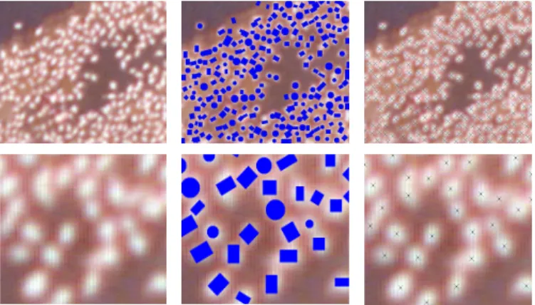
Figure 6 presents a result of the tree crown extraction by our multi-marked point process model. The main goal in this application is to count trees in large forest scenes for extracting statistics on the density of the stem. Although the shapes of trees are only roughly approximated by circles and rectangles, the trees are accurately detected. Even if no ground truth is available for this application, the accuracy of the tree locations is practically the same as obtained by [10] with elliptical objects to represent the trees. This new model allows the reduction of computational time by almost a factor three compared to [10] (77sec vs 212sec for the 240 × 350 pixel image in Figure 6).

The evolution of the object configuration during the jump-diffusion process is shown in Figure 7. At the beginning of the algorithm, i.e. when the temperature is high (red), the process explores the subspaces. Step by step, the configurations with a low energy are favored. At this exploration stage, the jump dynamic plays an important role by specifying both the number and the

Fig. 6. Tree crown extraction. (the upper row, from left to

right) The original aerial image c°IFN, our result, and the result by [10]; (the bottom row) the associated crops.

Fig. 7. Optimization process. (the upper row) Evolution of the object configuration from the initial temperature (red) to the final one (blue); (the bottom row) graphs of energy and number of objects in function of the iterations during jump-diffusion process.

type of objects. At low temperature (blue), the object configuration belongs to a subspace being close to the optimal one, and the number of objects in the scene does not evolve very much. The diffusion dynamic is useful at this stage mainly to perform a detailed adjustment of the object parameters. This dynamic is clearly faster than a single jump process with a perturbation kernel since the exploration is directed by the gradient of the energy (and not by a random search). Graphs in Figure 7 describe how the energy and the number of objects change in function of the number of iterations.

The bird detection problem is similar to the tree crown extraction: counting Flamingos in large colonies during the breeding season from large aerial images. Figure 8 presents results on a dense bird population which

Fig. 8. Bird detection. (the upper row, from left to right) The original aerial image c°Tour du Valat, our result, and ground truth; (the bottom row) the associated crops.

are qualitatively close to those obtained in [15] using a specialized marked point process with elliptical objects. The missed bird rate 3.7%, in Table 2, is comparable to the rate 2.1% obtained by the specialized bird detection model [15]. The missed birds mainly correspond to cases where a proposed object overlaps two close birds as we can see on the cropped result presented in Figure 8. The over-detection rate is quite low (< 3%) in both the models. Our model allows us to gain 25% in terms of computational time compared to [15] that uses an improved Birth-and-Death algorithm specially designed for the population counting problems.

The efficiency of the diffusion dynamics in our model is confirmed by experiments that substitute the diffu-sion stage by a uniform perturbation kernel added to our jump dynamics. Results in Table 2 underline that the diffusion dynamics is clearly both faster and more accurate than the use of a uniform perturbation kernel.

TABLE 2

Bird extraction evaluation in terms of detection rates and computing time (image size:560 × 496pixels).

missed over-detected computing time model with 3.7% 2.9% 290 sec Jump-Diffusion

model with 6.2% 4.4% 840 sec Jump

specialized bird 2.1% 2.0% 380 sec detection model[15]

5.2 Structure extraction

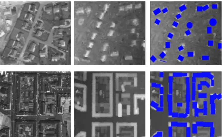
Figures 9 and 10 present results of line network and building extractions from aerial images. The obtained structures are globally slightly less accurate than those obtained by the specialized marked point processes. The road network extraction results cannot be considered as a final representation since the detected objects are not connected (contrary to [12] where special complex interactions had been defined to link the segments).

However, the detected objects are mainly lines and bands which are well fitted to roads or rivers. These objects provide a rough pattern of the network and are suf-ficiently informative to make it possible to extract the global network on the basis of their subsequent analysis (e.g. post-processing based on vectorization in order to connect the objects found). The results in Figure 9 are similar to those obtained by the active contour model presented in [37]. Our method is clearly faster than both the specialized marked point process and active contour models [12], [37] (See Table 3). Moreover, these two models have a sensitive and complex parameter tuning (more than 10 parameters for each one) compared to our algorithm.

Fig. 9. Line network extraction. (from top to bottom) Aerial images c°CNES/BRGM/IGN, the ground truth, results by our method, by [12], and by [37].

The building extraction is also workable but the object localization remains very rough compared to the spe-cialized model in [11]. This is mainly because of the over simplified data term in Eq. (7) that accounts for signal homogeneity inside and outside the object. Such a term is not relevant to this application since most of the building areas are heterogeneous due to non-flat

TABLE 3

Computing time for the line network extraction results presented on Figure 9 with a 2Ghz processor.

images our model mpp model[12] hoac model[37]

road (left) 235 sec 75 min 30 min 512 × 512 pix

river (middle) 107 sec 45 min 10 min 364 × 320 pix

road2 (right) 380 sec 155 min 60 min 892 × 652 pix

roofs. A term based on border discontinuity could be more efficient for this specific application. However, the proposed method detects main elements of the buildings and is clearly faster than the specialized marked point process in [11]: 30 minutes vs 2 hours on a 0.3 km2dense urban area using a 3 GHz processor.

Fig. 10. Building extraction. (from left to right) Peri-urban and dense urban aerial images c°IGN, the associated DEMs, and our results.

5.3 Texture representation

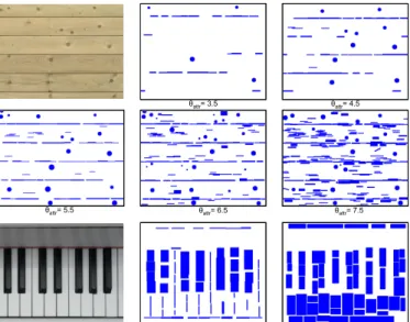
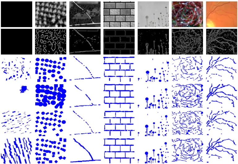
We also tested the proposed method on a number of natural textures in order to evaluate its potentialities for representing them by geometric objects. Representing textures is a partial texture reconstruction where we aim to extract texture components of interest so that they can be visual or/and statistically identified. The choice of the data measure (See Section 3.2.1) is important then for extracting the structures of interest. Such de-scriptions provide useful information for discriminated textures, even if it remains less detailed than texture synthesis methods [7], [8], [9]. The results (some of them are presented in Figure 11) are quite promising. The obtained descriptions reconstruct the overall rough structure and reveal interesting fine details on a large range of textures. Various spatially homogeneous and heterogeneous textures are successfully represented even with a chosen simple library of objects. Some natural textures perceived under spatially variant illumination and reflectance (see e.g. the metal grid and tile roof examples) are usually difficult to describe, and often

Fig. 11. Examples of natural texture representations in terms of geometrical objects.

require specific advanced techniques such as in [38]. Our method is particularly interesting for representing such textures since the fitting of objects does not depend on illumination effects. Various scales of details can be extracted in the texture structures (see e.g. the piano keyboard where the black keys are described by bands and the white key contours are represented by lines). The four last examples in Figure 11 show the limits of our model with respect to structure descriptions. In order to improve such representations, it is necessary to develop a more general energy function taking into account, in particular, typical object deviations and strong noise in

the textures (see e.g. the stone ornament and rose results). In terms of occurrence, lines and bands are the most frequent object types in the obtained texture represen-tations. They allow us to describe a large range of linear and areal structures. Rectangles and circles, which are bounded areal descriptors, are mainly selected to describe isolated components of textures. In particular, these two object types lead to convincing results on counting population problems. The three other types are less frequent, and are used in more specific structures such as metal grids.

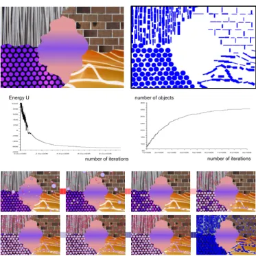
Figure 12 presents both the result obtained for an im-age with five different textures and the corresponding evolution of the object configuration during the jump-diffusion process. Even if the objects are disconnected (see e.g. brick wall or rays) and not correctly selected in some locations (see e.g. some rectangles in the disk grid), the obtained description in terms of objects clearly shows five different object layouts, and underlines good potentialities for subsequent texture discrimination and segmentation. In particular, it would be interesting to combine such object-based representations with Markov Gibbs random field models which are mostly used on the pixel-wise intensities [39] and thus do not explicitly take into account shapes and relative locations of de-picted characteristic objects. In order to deal with more complicated textures and have a description level similar to filter bank methods [40], affine-invariant descriptors [41], or wavelet based parametric models [42], the object library has to be extended by introducing new relevant shapes, especially general curved shapes or/and micro-structure elements [43]. In this perspective, learning of dominant micro-structure elements such as e.g. in [44] is promising for the automatic selection of relevant objects from training images.

Figure 13 shows a comparison with the multi-layer texton model presented in [8]. Our approach provides a good representation of the textures with few false alarms as we can see for example on the crack image where many small lines have been extracted. However it remains limited in terms of description compared to the multi-layer texton model which allows the complete reconstruction of textures by sampling different layers of texture components. The interesting point consists in comparing both the models on textures composed of a foreground layer and a homogeneous background. In this case, our model can reconstruct the textures (see the third row on Figure 13 where both the extracted objects and background have been colored using the associated intensity means in the texture image), and the obtained results are very satisfactory for a non specialized texture reconstruction model. The localization accuracy we ob-tained is similar to that of the texton model as we can see for example on the crack results. However, the brick results show that the object connection quality of the texton model is clearly better than the one we obtain. In Section 6, we propose additional object interactions which will allow the improvement of this point. The

Fig. 12. Texture representation. (the upper row, from left

to right) Original image and our result; (the middle row)

graphs of energy and number of objects in function of the iterations during jump-diffusion process; (the bottom

row) evolution of the object configuration from the initial

temperature (red) to the final one (blue).

Fig. 13. Comparison with the texton model [8]. (from top

to bottom) Textures c°UCLA, our results, our associated reconstructed textures, the foreground and background texton extractions by [8] and the associated reconstructed textures c°UCLA.

cheetah skin results underline the limits of our model when several texton layers are required for describing various texture components (i.e. big dark and small grey spots). On the contrary, the texton model leads to an accurate reconstruction on such a multi-component texture.

Figure 14 presents the impact of the model parameter θattr on the results. This parameter, which tunes the

sensitiveness of data fitting, plays an important role in the final number of objects describing the image. A low value (e.g. 3.5 or 4.5) provides representations containing few accurately localized objects. On the contrary, a high value (such as 6.5 or 7.5) gives much more dense de-scriptions but with many roughly detected objects. In our experiments, θattrhas been tuned in the interval [5.1, 5.8]

which constitutes a good compromise between the level of details of the representation and the accuracy of the object locations. An automatic estimation of θattr from a

given image represents a challenging but interesting per-spective. Several kinds of information such as the signal to noise ratio or signal co-occurrence repetitiveness in the image could be taken into account for this estimation. Figure 14 also shows results using different data fitting measures.

Fig. 14. Impact of the model parameters. (the upper rows) Impact of θattr on a natural texture representation; (the

bottom row) impact of thedbrightandddarkmeasures.

6

I

-TERACTIONS

As mentioned in Section 3.2.2, introducing specific regu-larization constraints directly impacts on three points: (i) more complex parameter tunings, (ii) higher computing times, and (iii) loss of the model generality level. How-ever, such interactions bring helpful structural knowl-edge in some applications and can allow us to obtain better results by reducing the True Negatives and the False Positives. In this section, we discuss the interest of

inserting new types of object interactions in the energy model (see Eq. 5) and analyze their efficiency on various applications.

6.1 New object interactions

According to the experiments realized in Section 5, some results suffer from both a lack of object connection and an approximated object alignment, especially for line network extraction and texture representation. We propose to introduce these two additional interactions in our energy model in the following.

6.1.1 Inter-connection

Such an interaction type can be efficiently modeled from the non-overlapping constraint defined in Section 3.2.2 by favoring the connected objects in keeping the high overlaps penalize. To to so, we introduce the parameter γattr>1 which makes attractive (respectively repulsive)

weak (resp. high) object overlaps. The modified prior is expressed as follows:

Rc_k(x) = X

xi,xj∈x

(eκg(xi,xj)_{− γ}

attr) (15)

γattr controls the balance between attraction and

repul-sion in function of object overlapping. For example, if we want to favor configurations with an overlap up to 20%, we will take γattr= exp 0.2κ.

6.1.2 Mutual alignment

This term aims at penalizing the orientation changes of neighboring elements. It is given by:

Ra_k(x) = X

xi,xj∈x

(eκg(xi,xj)_{− 1) + λ} X

xi,xj∈x

A(xi, xj) (16)

where A(xi, xj) measures the mutual alignment of the

objects xi and xj using a L1

2 norm. A(., .) takes values

in [0, 1] and λ is a parameter weighting the importance of the object alignment with respect to the non-overlapping criterion. When xi or xj is a rotation-invariant object

(i.e. a circle), we impose A(xi, xj) = a where a ∈ [0, 1]

is a parameter allowing us to tune the occurrence of rotation-invariant object with respect to non rotation invariant objects. This additional parameter is necessary for modeling alignment constraints when the object li-brary contains rotation-invariant objects.

6.1.3 Inter-connection and mutual alignment associa-tion

This prior is a simple combination of both the interaction types detailed above:

Rac_k (x) = X xi,xj∈x (eκg(xi,xj)_{− γ} attr) + λ X xi,xj∈x A(xi, xj) (17) These three priors remain more general than those used in the specialized marked point processes and are mod-eled by less parameters. In addition, they are differen-tiable which is necessary to perform diffusion dynamics.

Compared to the original model presented in Section 3, the new energies are more complex and additional computing time is required to optimize them.

6.2 Model complexity and efficiency

The prior terms detailed above have been tested on various applications. Figure 15 presents the obtained results and comparisons to the initial model and the conventional Canny edge detector [45]. Even if the Canny detector suitably extracts shapes of interest in the presented textures, such an approach is limited to pixel analysis and does not take into account the object concept. Such an edge extraction is interesting to evalu-ate the complexity of the presented images in terms of boundary accuracy, noise and shape irregularity. Simulations without data (See first column on Figure 15) show right behaviors of the proposed priors in accordance with the expectation. The inter-connection term, Rc

k, allows us to slightly improve the results by

reducing the false alarms but remains insufficient for decreasing the true negative (See the road extraction result for example). This term is clearly not adapted to population counting problems as we can see on the tree extraction result where objects are enlarged to be con-nected together. On the contrary, the mutual alignment term gives an interesting result for this application and allows us to extract more efficiently such a grid structure by regularizing the object orientation. The interest of Rc_k is quite limited for the others applications. The last term, Rac

k , gives the best results for almost all the tested

images. The combination of connection and alignment constraints strongly reduces the number of false positive and true negative as we can see on road and blood vessel extraction. This prior also brings accurate texture representations and allows us to clearly improve the results on complex cases such as the flower. Table 4 evaluates the efficiency of these three priors in terms of parameter tuning and computing time. The term Rac

k , which gives the best results, also corresponds to

the most complex parameter tuning and the highest computing time. Depending on the application context, the initial model is preferred since the tuning of the four parameters by trial and error requires time and expertise.

TABLE 4

Prior efficiency evaluation.

interactions parameters extra computing time Rc

k, connection θattr, γattr 32%

Ra

k, alignment and θattr, λ, a 48%

non-overlapping Rac

k , connection θattr, γattr, λ, a 91%

and alignment

7

C

The proposed new approach based on a multi-marked point process model allows the representation of images

in terms of simple geometric features. Although the obtained results are generally slightly less accurate than those provided by the specialized marked point process models, our approach possesses several interesting char-acteristics. First, it is more general and works efficiently on various applications such as counting population problems, structure reconstruction from remotely sensed images, and natural texture representation whereas the conventional approaches needed to exploit specialized models for each problem. Moreover, we have proposed an efficient Jump-Diffusion algorithm adapted to marked point processes that allows us to strongly reduce com-putational time with respect to the classical jump tech-niques. Finally, we have decreased the number of tuning parameters by formulating a global model and have discussed the compromise between model complexity and efficiency by analyzing the impact of additional object interactions in the model.

However, our approach is limited by the content of the mark library: the current set in Figure 3 cannot in principle provide relevant representations of complex structures such as multiple junctions or random curved shapes. In the future, we will extend the mark library and develop probabilistic models and techniques for automatic selection of relevant ”basic” objects from a given collection of training images. Another perspective would be to improve the data term of our model by using both a more efficient differentiable and quickly computable measure which takes into account specific information such as noise models or contour accuracy, and to provide an automatic estimation of the data fitting sensitiveness parameter.

A

Computation of the birth-and-death kernel

Let us consider a birth, chosen with a probability pb,

from object configurations x = (xp)p∈[1,n(x)] to y =

x∪ {xn(x)+1} where xn(x)+1 is the new added object

chosen randomly on the object space. The ratio of the kernels in the acceptance rate equation (see Eq. 11) is then expressed by:

QBD(y → x) QBD(x → y) =pd pb ν(K) n(x) + 1 (18)

where pb (respectively, pd= 1 − pb) is the probability of

choosing a birth (respectively, a death), and ν(.) is the intensity of the reference Poisson process (See Section 2.1). In our model, the probabilities of choosing a birth and a death are the same (i.e. pd= pb).

Let us consider now a death from object configurations x= (xp)p∈[1,n(x)]to y = x−{xi} where xiis the removed

object chosen randomly in the object configuration x. By the reversible assumption, the kernel ratio of the death is given by: QBD(y → x) QBD(x → y) = pb pd n(x) ν(K) (19)

Fig. 15. Efficiency of the various interactions. (from top to down) Images, Canny edge detector, results using the original model, the connection, the alignment, and the connection/alignment interaction priors. The number of objects on simulations without data (first column) has been voluntarily upper bounded in order to avoid infinite grouping of objects and then to have comprehensible results.

Computation of the switching kernel

Let us consider a jump from an object xi of type Tm(for

example, a circle) to an object bxiof type Tn(for example,

a rectangle) such that the current object configuration x = (xp)p∈[1,n(x)] is perturbed into the configuration

y = x − {xi} ∪ bxi. We then create a bijection between

the parameter spaces of the object types Tm and Tn:

xi is completed by auxiliary variables umn simulated

under a law ϕmn(.) to provide (xi, umn), and bxi by

vnm∼ ϕnm(.) into ( bxi, vmn) such that the mapping Ψmn

between (xi, umn) and ( bxi, vmn) is a bijection :

( bxi, vmn) = Ψmn(xi, umn) (20)

The ratio of the kernels in the acceptation ratio (see Eq. 11) is then expressed by:

QS(y → x) QS(x → y) = Jnmϕnm(vnm) Jmnϕmn(umn) ¯ ¯ ¯ ¯ ∂Ψmn(xi, umn) ∂(xi, umn) ¯ ¯ ¯ ¯ (21) where Jmn corresponds to the probability of choosing a

jump from the object type Tm to the object type Tn. In

our case, the object types are equiprobable. It implies

Jnm = Jmn. In our experiments, the mark library is

composed of seven object types having five different parameter sets shown in Table 1. Then, 52 _{− 5 = 20}

bijections and associated completion parameters must be computed.

Let us consider, for example, a jump from a circle (denoted T1) to a rectangle (denoted T2). We move from

xi= (cx, cy, r) to bxi = (cx, cy, L, l, θ). The parameters cx

and cy specifying the center of mass exist in both the

object types. Moreover, we can define a linear transfor-mation between the radius r ∈ [rmin, rmax] of the circle

and the length L ∈ [Lmin, Lmax] of the rectangle such

as L = Lmax−Lmin

rmax−rminr+

Lminrmax−Lmaxrmin

rmax−rmin . Thus, we need

to complete the object type T1 by u1 2 = (l, θ). We then

obtain bxi= Ψ1 2(xi, u1 2) with

Ψ1 2(X) =

 

Id2 0 02,2

02,1 L_rmax_max−−Lrminmin 02,1

02,2 0 Id2   X +   01,2 Lminrmax−Lmaxrmin

rmax−rmin

01,2

  (22)

where Idi and 0i,j are the identity matrix of size i and

the zero matrix of size i×j, respectively. Finally, we have ¯ ¯ ¯∂Ψ1 2(xi,u1 2) ∂(xi,u1 2) ¯ ¯ ¯ = Lmax−Lmin

rmax−rmin. The completion parameters

u1 2 are chosen following uniform distributions on the

parameter spaces.

Computation of the energy gradient

Let p denote a parameter of the object xi of the object

configuration x ∈ Ck. Then, the energy derivative with

respect to p is given by:

dUk(x) dp = P xk∈x dd(xk) dp + P xk,xl∈x d(eκg_(xk,xl)−1) dp = d(xi) ′ +P j∼i κg(xi, xj)′eκg(xi,xj) (23) where (.)′

= d_{d p}(.) and the notation j ∼ i corresponds to the set of objects xj such as g(xi, xj) 6= 0 (i.e. the

neighboring objects of xi). The data term is as follows:

d(xi) ′ = σ 2 in ′ + σ2 out ′ 2S(d(xi) + θattr)(min− mout)2 × " 1 − µ_S′ S + 2 min′− mout′ min− mout ¶ σ2 in+ σ2out+ ǫ σ_in2′+ σ2 out ′ # (24) If min= mout, a hardcore is associated with the energy

which means the object configuration is forbidden. The derivatives of the statistical parameters used in Eq. 24 are given by the following expressions:

min′= −Sin ′ min+ 1 S_in Z ∂Ωin I (25) mout′= −Sout ′ mout+ 1 S_out Z ∂Ωout I (26) σ2_in′= − Sin ′ σ_in2+ 1 Sin ·Z ∂Ωin (I − min)2− 2 Z Ωin min′(I − min) ¸ (27) σ2_out′= − Sout ′ σ_out2 + 1 Sout × ·Z ∂Ωout (I − mout)2− 2 Z Ωout mout′(I − mout) ¸ (28) where I is the intensity of the image, Ωin and Ωout are

the inside and outside domain, respectively, and Sinand

S_{out are the area of these domains. If we consider the} energy derivative with respect to the center of mass and orientation object parameters, the computation is simplified since the area of the object does not depend on these parameters (i.e. S′

= Sin ′ = Sout ′ = 0).

A

The first author is grateful to the French Defense Agency (DGA) for financial support. The authors thank the reviewers for the helpful comments and suggestions, the French Mapping Agency (IGN), the French Forest Inventory (IFN), the French Space Agency (CNES), the French Geological Survey (BRGM) and the Tour du Valat for the aerial and satellite images; CGtextures and the UCLA Department of Statistics for the texture images; DRIVE database for the retinal images.

R

[1] G. Winkler, Image Analysis, Random Fields and Markov Chain Monte

Carlo Methods: A Mathematical Introduction. Springer, 1995.

[2] S. Li, Markov Random Field Modeling in Computer Vision. Springer-Verlag, 1995.

[3] W. Hastings, “Monte Carlo sampling using Markov chains and their applications,” Biometrica, vol. 57(1), pp. 97–109, 1970. [4] P. Green, “Reversible Jump Markov Chains Monte Carlo

compu-tation and Bayesian model determination,” Biometrika, vol. 82(4), pp. 711–732, 1995.

[5] A. Dick, P. Torr, and R. Cipolla, “Modelling and interpretation of architecture from several images,” International Journal of Computer

Vision, vol. 60(2), pp. 111–134, 2004.

[6] F. Lafarge, X. Descombes, J. Zerubia, and M. Pierrot-Deseilligny, “Building reconstruction from a single DEM,” in IEEE Proc.

Com-puter Vision and Pattern Recognition, Anchorage, United States, 2008.

[7] Y. Wu, S. Zhu, and C. Guo, “Statistical modeling of texture sketch,” in European Conference Computer Vision, Copenhagen, Denmark, 2002.

[8] C. E. Guo, S. Zhu, and Y. Wu, “Modeling visual patterns by inte-grating descriptive and generative models,” International Journal of

Computer Vision, vol. 53, no. 1, pp. 5–29, 2003.

[9] G. Gimel’farb, Image Textures and Gibbs Random Fields. Kluwer Academic, 1999.

[10] G. Perrin, X. Descombes, and J. Zerubia, “Adaptive simulated annealing for energy minimization problem in a marked point pro-cess application,” in Proc. Energy Minimization Methods in Computer

Vision and Pattern Recognition, St Augustine, United States, 2005.

[11] M. Ortner, X. Descombes, and J. Zerubia, “Building outline extrac-tion from Digital Elevaextrac-tion Models using marked point processes,”

International Journal of Computer Vision, vol. 72, no. 2, pp. 107–132,

2007.

[12] C. Lacoste, X. Descombes, and J. Zerubia, “Point processes for unsupervised line network extraction in remote sensing,” IEEE

Trans. Pattern Analysis and Machine Intelligence, vol. 27, no. 10, pp.

1568–1579, 2005.

[13] O. Tournaire, N. Paparoditis, and F. Lafarge, “Rectangular road marking detection with marked point processes,” in Proc. conference

on Photogrammetric Image Analysis, Munich, Germany, 2007.

[14] K. Sun, N. Sang, and T. Zhang, “Marked point process for vascular tree extraction on angiogram,” in Proc. Energy Minimization Methods

in Computer Vision and Pattern Recognition, Ezhou, China, 2007.

[15] S. Descamps, X. Descombes, A. B´echet, and J. Zerubia, “Automatic flamingo detection using a multiple birth and death process,” in Proc. IEEE International Conf. on Acoustics, Speech and Signal

Processing, Las Vegas, United States, 2008.

[16] M. Van Lieshout, “Markov point processes and their applica-tions,” in Imperial College Press, London, 2000.

[17] C. Geyer and J. Moller, “Simulation and likelihood inference for spatial point processes,” Scandinavian Journal of Statistics, vol. Series B, no. 21, pp. 359–373, 1994.

[18] M. Metropolis, A. Rosenbluth, A. Teller, and E. Teller, “Equation of state calculations by fast computing machines,” Journal of Chemical

Physics, vol. 21, pp. 1087–1092, 1953.

[19] S. Geman and C. Huang, “Diffusion for global optimization,”

SIAM Journal on Control and Optimization, vol. 24(5), pp. 131–143,

1986.

[20] U. Grenander and M. Miller, “Representations of Knowledge in Complex Systems,” Journal of the Royal Statistical Society, vol. 56, no. 4, pp. 1–33, 1994.

[21] F. Lafarge and G. Gimel’farb, “Texture representation by geomet-ric objects using a jump-diffusion process,” in Proc. British Machine

Vision Conference, Leeds, United Kingdom, 2008.

[22] A. Baddeley and M. Van Lieshout, “Stochastic geometry models in high-level vision,” Statistics and Images, vol. 1, pp. 233–258, 1993. [23] H. Rue and A. Syverseen, “Bayesian object recognition with baddeleys delta loss,” Advances in Applied Probability, vol. 30, pp. 64–84, 1998.

[24] A. Pievatolo and P. Green, “Boundary detection through dynamic polygons,” Journal of the Royal Statistical Society, vol. 60, no. B, pp. 609–626, 1998.

[25] S. Geman and D. Geman, “Stochastic relaxation, Gibbs distribu-tions and the Bayesian restoration of images,” IEEE Trans. Pattern

Analysis and Machine Intelligence, vol. 6, no. 6, pp. 721–741, 1984.

[26] M. Ortner, X. Descombes, and J. Zerubia, “A marked point process of rectangles and segments for automatic analysis of digital eleva-tion models,” IEEE Trans. Pattern Analysis and Machine Intelligence, vol. 30, no. 1, pp. 105–119, 2008.

[27] T. Wu, G. Xia, and S. Zhu, “Compositional boosting for computing hierarchical image structures,” in IEEE Proc. Computer Vision and

Pattern Recognition, Minneapolis, United States, 2007.

[28] A. Desolneux, L. Moisan, and J.-M. Morel, From Gestalt Theory to

Image Analysis: A Probabilistic Approach. Springer, 2008.

[29] A. Srivastava, M. Miller, and U. Grenander, “Multiple target direction of arrival tracking,” IEEE Trans. Signal Processing, vol. 43, no. 5, pp. 282–285, 1995.

[30] A. Srivastava, U. Grenander, G. Jensen, and M. Miller, “Jump-Diffusion Markov processes on orthogonal groups for object pose estimation,” Journal of Statistical Planning and Inference, vol. 103, no. 1/2, pp. 15–37, 2002.

[31] F. Han, Z. Tu, and S. Zhu, “Range Image Segmentation by an Effective Jump-Diffusion Method,” IEEE Trans. Pattern Analysis and

Machine Intelligence, vol. 26, no. 9, pp. 1138–1153, 2004.

[32] P. Van Laarhoven and E. Aarts, Simulated Annealing : Theory and

Applications. Boston, United States: D. Reidel, 1987.

[33] P. Salamon, P. Sibani, and R. Frost, Facts, Conjectures, and

Improve-ments for Simulated Annealing. Philadelphia, United States: SIAM Monographs on Mathematical Modeling and Computation, 2002. [34] J. Varanelli, “On the aacceleration of the simulated annealing,”

Ph.D. dissertation, University of Virginia, Charlottesville, United States, 1996.

[35] H. Haario and E. Saksman, “Simulated annealing process in general state space,” Advances in Applied Probability, no. 23, pp. 866–893, 1991.

[36] S. White, “Concepts of scale in simulated annealing,” in Proc. IEEE

International Conference on Computer Design, 1984.

[37] M. Rochery, I. Jermyn, and J. Zerubia, “Higher Order Active Contours,” International Journal of Computer Vision, vol. 69, no. 1, pp. 27–42, 2006.

[38] M. Chantler, M. Petrou, A. Penirsche, M. Schmidt, and G. McGun-nigle, “Classifying surface texture while simultaneously estimating illumination direction,” International Journal of Computer Vision, vol. 62(1-2), pp. 83–96, 2005.

[39] G. Gimel’farb, “Texture modeling by multiple pairwise pixel interactions,” IEEE Trans. Pattern Analysis and Machine Intelligence, vol. 18, no. 11, pp. 1110–1114, 1996.

[40] M. Varma and A. Zisserman, “A statistical approach to texture classification from single images,” International Journal of Computer

Vision, vol. 62(1-2), pp. 61–81, 2005.

[41] S. Lazebnik, C. Schmid, and J. Ponce, “A sparse texture represen-tation using local affine regions,” IEEE Trans. Pattern Analysis and

Machine Intelligence, vol. 27, no. 8, pp. 1265–1278, 2005.

[42] J. Portilla and E. Simoncelli, “A parametric texture model based on joint statistics of complex wavelet coefficients,” International

Journal of Computer Vision, vol. 40, no. 1, pp. 49–71, 2000.

[43] B. Julesz, “Textons, the elements of texture perception and their interactions,” Nature, vol. 290, pp. 91–97, 1981.

[44] S. Zhu, C. E. Guo, Y. Wang, and Z. Xu, “What are textons?”

International Journal of Computer Vision, vol. 62, no. 1/2, pp. 121–143,

2005.

[45] J. Canny, “A computational approach to edge detection,” IEEE

Trans. Pattern Analysis and Machine Intelligence, vol. 8, no. 6, pp.

679–698, 1986.

PLACE PHOTO HERE

Florent Lafarge received the BSc degree in aeronautics from the French School of Aero-nautics in 2004 and the MSc degree in applied mathematics from the University of Toulouse, France, in the same year. From 2004 to 2007, he prepared the PhD degree at the INRIA and at the French Mapping Agency. He received the PhD degree in applied mathematics from the Ecole Nationale Sup ´erieure des Mines de Paris, in 2007. From 2007 to 2008, he was a research visitor at the University of Auckland, New Zealand. He is now working as a postdoctoral researcher at the CERTIS laboratory of the Ecole Nationale des Ponts et Chauss ´ees, Paris, France. His research interests are probabilistic modeling in image processing, stereo vision techniques and 3D reconstruction processes.

PLACE PHOTO HERE

Georgy Gimel’farb received the M.S. degree (with honors) in electrical engineering from the Kiev Polytechnic Institute, Ukraine, in 1962, the Ph.D. degree in engineering cybernetics from the Institute of Cybernetics, Academy of Sciences of the Ukraine, in 1969, and the D.Sc.(Eng) degree in control in engineering from the Higher Certifying Commission of the USSR, Moscow, Russia, in 1991. After a long time with the Institute of Cybernetics and the International Training and Research Centre of Information Technologies and Systems (Kiev, Ukraine), since July 1997 he has been with the Department of Computer Science of the University of Auckland (Auckland, New Zealand), where he is currently an Associate Professor of computer science. His research interests are in the areas of prob-abilistic image modeling, texture analysis, computational stereo vision, and 3D image matching and recognition. Dr. Gimel′_{farb was a Track} Co-chair of the 19th_{International Conference on Pattern Recognition (ICPR}

2008), Tampa, Florida, USA. He is a recipient of the 1997 State Award of Ukraine in Science and Technology.

PLACE PHOTO HERE

Xavier Descombes received the bachelors de-gree in telecommunications from the Ecole Na-tionale Superieure des Telecommunications de Paris (ENST) in 1989, the master of science de-gree in mathematics from the University of Paris VI in 1990, the PhD degree in signal and image processing from the ENST in 1993, and the ”habilitation” from the University of Nice-Sophia Antipolis in 2004. He has been a postdoctoral researcher at ENST in 1994, at the Katolieke Universitat Leuven in 1995, and at the Institut National de Recherche en Informatique et en Automatique (INRIA) in 1996 and a visiting scientist in the Max Planck Institute of Leipzig in 1997. He is currently at INRIA as a research director. His research interests include Markov Random Fields, stochastic geometry, and stochastic modeling in image processing.