SLIDE: A Useful Special Case of the CARDPATH Constraint

HAL Id: lirmm-00329876

https://hal-lirmm.ccsd.cnrs.fr/lirmm-00329876

Submitted on 13 Oct 2008

HAL is a multi-disciplinary open access

archive for the deposit and dissemination of

sci-entific research documents, whether they are

pub-lished or not. The documents may come from

teaching and research institutions in France or

abroad, or from public or private research centers.

L’archive ouverte pluridisciplinaire HAL, est

destinée au dépôt et à la diffusion de documents

scientifiques de niveau recherche, publiés ou non,

émanant des établissements d’enseignement et de

recherche français ou étrangers, des laboratoires

publics ou privés.

SLIDE: A Useful Special Case of the CARDPATH

Constraint

Christian Bessière, Emmanuel Hébrard, Brahim Hnich, Zeynep Kiziltan, Toby

Walsh

To cite this version:

Christian Bessière, Emmanuel Hébrard, Brahim Hnich, Zeynep Kiziltan, Toby Walsh. SLIDE: A

Use-ful Special Case of the CARDPATH Constraint. ECAI: European Conference on Artificial Intelligence,

Jul 2008, Patras, Greece. pp.475-479. �lirmm-00329876�

SLIDE: A Useful Special Case

of the CARDPATH Constraint

Christian Bessiere

and Emmanuel Hebrard

and Brahim Hnich

and Zeynep Kiziltan

and Toby Walsh

Abstract. We study the CARDPATHconstraint. This ensures a given constraint holds a number of times down a sequence of variables. We show that SLIDE, a special case of CARDPATHwhere the slid constraint must hold always, can be used to encode a wide range of sliding sequence constraints including CARDPATHitself. We con-sider how to propagate SLIDEand provide a complete propagator for CARDPATH. Since propagation is NP-hard in general, we identify special cases where propagation takes polynomial time. Our experi-ments demonstrate that using SLIDEto encode global constraints can be as efficient and effective as specialised propagators.

1

INTRODUCTION

In many scheduling problems, we have a sequence of decision vari-ables and a constraint which applies down the sequence. For exam-ple, in the car sequencing problem, we need to decide the sequence of cars on a production line. We might have a constraint on how often a particular option is met (e.g. 1 out of 3 cars can have a sun-roof). As a second example, in a nurse rostering problem, we need to decide the sequence of shifts worked by nurses. We might have a constraint on how many consecutive night shifts any nurse can work. Such con-straints have been classified as sliding sequence concon-straints [7]. To model such constraints, we can use the CARDPATHconstraint. This ensures that a given constraint holds a number of times down a se-quence of variables [5]. We identify a special case of CARDPATH which we call SLIDE, that is interesting for several reasons. First, many sliding sequence constraints, including CARDPATH, can easily be encoded using this special case. SLIDEis therefore a “general-purpose” constraint for encoding sliding sequencing constraints. This is an especially easy way to provide propagators for such global con-straints within a constraint toolkit. Second, we give a propagator for enforcing generalised arc-consistency on SLIDE. By comparison, the previous propagator for CARDPATHgiven in [5] does not prune all possible values. Third, SLIDEcan be as efficient and effective as spe-cialised propagators in solving sequencing problems.

1_{LIRMM (CNRS / U. Montpellier), France, email: bessiere@lirmm.fr.} Sup-ported by the ANR project ANR-06-BLAN-0383-02.

2_{4C, UCC, Ireland, email: ehebrard@4c.ucc.ie.}

3 _{Izmir Uni. of Economics, Turkey, email: brahim.hnich@ieu.edu.tr.} Sup-ported by the Scientific and Technological Research Council of Turkey (TUBITAK) under Grant No. SOBAG-108K027.

4_{CS Department, Uni. of Bologna, Italy, email: zeynep@cs.unibo.it.} 5 _{NICTA and UNSW, Sydney, Australia, email: toby.walsh@nicta.com.au.}

Funded by the Australian Government’s Department of Broadband, Com-munications and the Digital Economy, and the ARC.

2

CARDPATH AND SLIDE CONSTRAINTS

A constraint satisfaction problem consists of a set of variables, each with a finite domain of values, and a set of constraints specifying allowed combinations of values for given sets of variables. We use capital letters for variables (e.g.X), and lower case for values (e.g. d). We write D(X) for the domain of variable X. Constraint solvers

typically explore partial assignments enforcing a local consistency property. A constraint is generalised arc consistent (GAC) iff when a variable is assigned any value in its domain, there exist compatible values in the domains of all the other variables of the constraint.

The CARDPATHconstraint was introduced in [5]. IfC is a

con-straint of arity k then CARDPATH(N, [X1, . . . , Xn], C) holds iff

C(Xi, . . . , Xi+k−1) holds N times for 1 ≤ i ≤ n − k + 1. For

example, we can count the number of changes in the type of shift with CARDPATH(N, [X1, . . . , Xn], 6=). Note that CARDPATH can

be used to encode a range of Boolean connectives sinceN ≥ 1

gives disjunction,N = 1 gives exclusive or, and N = 0 gives

nega-tion. We shall focus on a special case of the CARDPATHconstraint where the slid constraint holds always. SLIDE(C, [X1, . . . , Xn])

holds iffC(Xi, . . . , Xi+k−1) holds for all 1 ≤ i ≤ n − k + 1.

That is, a CARDPATHconstraint in whichN = n − k + 1. We

also consider a more complex form of SLIDEthat applies only ev-eryj variables. More precisely, SLIDEj(C, [X1, . . . , Xn]) holds iff

C(Xij+1, . . . , Xij+k) holds for 0 ≤ i ≤ n−k_j . By definition

SLIDEjforj = 1 is equivalent to SLIDE.

Beldiceanu and Carlsson have shown that CARDPATHcan encode a wide range of constraints like CHANGE, SMOOTH, AMONGSEQ and SLIDINGSUM[5]. As we discuss later, SLIDEprovides a simple way to encode such sliding sequencing constraints. It can also en-code many other more complex sliding sequencing constraints like REGULAR[16], STRETCH[13], and LEX[7], as well as many types of chanelling constraints like ELEMENT[19] and optimisation con-straints like the soft forms of REGULAR[20]. More interestingly, CARDPATHcan itself be encoded into a SLIDEconstraint. In [5], a propagator for CARDPATHis proposed that greedily constructs up-per and lower bounds on the number of (un)satisfied constraints by posting and retracting (the negation of) each of the constraints. This propagator does not achieve GAC. We propose here a complete prop-agator for enforcing GAC on SLIDE. SLIDEthus provides a GAC propagator for CARDPATH. In addition, SLIDEprovides a GAC prop-agator for any of the other global constraints it can encode. As our experimental results reveal, SLIDEcan be as efficient and effective as specialised propagators.

We illustrate the usefulness of SLIDE with the AMONGSEQ constraint which ensures that values occur with some given fre-quency. For instance, we might want that no more than 3 out of every sequence of 7 shift variables are a “night shift”. More

precisely, AMONGSEQ(l, u, k, [X1, . . . , Xn], v) holds iff between

l and u variables in every sequence of k variables take value

in the ground set v [8]. We can encode this using SLIDE. More precisely, AMONGSEQ(l, u, k, [X1, . . . , Xn], v) can be encoded

as SLIDE(D_l,uk,v, [X1, . . . , Xn]) where Dl,uk,v is an instance of the

AMONGconstraint [8].Dk,v

l,u(Xi, . . . , Xi+k−1) holds iff between l

andu variables take values in the set v. For example, suppose 2 of

every 3 variables along a sequenceX1. . . X5should take the value

a, where X1 = a and X2, . . . , X5 ∈ {a, b}. This can be encoded

as SLIDE(E, [X1, X2, X3, X4, X5]) where E(Xi, Xi+1, Xi+2)

en-sures two of its three variables takea. This SLIDEconstraint ensures thatE(X1, X2, X3), E(X2, X3, X4) and E(X3, X4, X5) all hold.

Note that each ternary constraint is GAC. However, enforcing GAC on the SLIDEconstraint setsX4= a as there are only two satisfying

assignments and neither haveX4 = b.

3

SLIDE WITH MULTIPLE SEQUENCES

We often wish to slide a constraint down two or more sequences of variables at once. For example, suppose we want to ensure that two vectors of variables,X1toXnandY1toYndiffer at every index. We

can encode such a constraint by interleaving the two sequences and sliding a constraint down the single sequence with a suitable offset. In our example, we simply post SLIDE2(6=, [X1, Y1, . . . , Xn, Yn]).

As a second example of sliding down multiple sequences of vari-ables, consider the constraint REGULAR(A, [X1, . . . , Xn]). This

en-sures that the values taken by a sequence of variables form a string accepted by a deterministic finite automatonA [16]. This global

con-straint is useful in scheduling, rostering and sequencing problems to ensure certain patterns do (or do not) occur over time. It can be used to encode a wide range of other global constraints including: AMONG [8], CONTIGUITY[15], LEXand PRECEDENCE[14].

To encode the REGULAR constraint with SLIDE, we intro-duce variables, Qi to record the state of the automaton. We

then post SLIDE2(F, [Q0, X1, Q1, . . . , Xn, Qn]) where Q0 is set

to the starting state, Qn is restricted to accepting states, and

F (Qi, Xi+1, Qi+1) holds iff Qi+1 = δ(Xi, Qi) where δ is the

transition function of the automaton. If we decompose this encoding into the conjunction of slid constraints, we get a set of constraints similar to [6]. Enforcing GAC on this encoding ensures GAC on REGULARand, by exploiting functionaliy ofF , takes O(ndq) time

whered is the number of values for Xiandq is the number of states

of the automaton. This is asymptotically identical to the specialised REGULARpropagator [16]. This encoding is highly competitive in practice with the specialized propagator [2].

One advantage of this encoding is that it gives explicit access to the states of the automaton. Consider, for example, a rostering problem where workers are allowed to work for up to three consecutive shifts. This can be specified with a simple REGULARconstraint. Suppose now we want to minimise the number of times a worker has to work for three consecutive shifts. To encode this, we can post an AMONG constraint on the state variables to count the number of times we visit the state representing three consecutive shifts, and minimise the value taken by this variable. As we shall see later in the exper-iments, the encoding also gives an efficient incremental propagator. In fact, the complexity of repeatedly enforcing GAC on this encoding of the REGULARconstraint down the whole branch of a backtracking search tree is justO(ndq) time.

4

SLIDE WITH COUNTERS

We may want to slide a constraint on a sequence of variables comput-ing a count. We can use SLIDEto encode such constraints by incre-mentally computing the count in an additional sequence of variables. Consider, for example, CARDPATH(N, [X1, . . . , Xn], C). For

sim-plicity, we considerk = 2 (i.e., C is binary). The generalisation to

otherk is straightforward. We introduce a sequence of integer

vari-ablesMiin which to accumulate the count. We encode CARDPATH

as SLIDE2(G, [M1, X1, . . . , Mn, Xn]) where M1 = 0, Mn = N ,

andG(Mi, Xi, Mi+1, Xi+1) is defined as: if C(Xi, Xi+1) holds

thenMi+1 = Mi+ 1, otherwise Mi+1 = Mi. GAC on SLIDE

ensures GAC on CARDPATH.

As a second example, consider the STRETCH constraint [13]. Given variables X1 to Xn taking values from a set of shift

types τ , a set π of ordered pairs from τ × τ , and functions shortest(t) and longest(t) giving the minimum and maximum

length of a stretch of typet, STRETCH([X1, . . . , Xn]) holds iff each

stretch of typet has length between shortest(t) and longest(t);

and consecutive types of stretches are in π. We can encode

STRETCHas SLIDE2(H, [X1, Q1, . . . , Xn, Qn]) where Q1 = 1 and

H(Xi, Xi+1, Qi, Qi+1) holds iff (1) Xi= Xi+1,Qi+1= 1 + Qi,

andQi+1 ≤ longest(Xi); or (2) Xi 6= Xi+1,hXi, Xi+1i ∈ π,

Qi≥ shortest(Xi) and Qi+1 = 1. GAC on SLIDEensures GAC on STRETCH.

5

OTHER EXAMPLES OF SLIDE

There are many other examples of global constraints which we can encode using SLIDE. For example, we can encode LEX [7] us-ing SLIDE. LEXholds iff a vector of variables[X1..Xn] is

lexico-graphically smaller than another vector of variables[Y1..Yn]. We

introduce a sequence of Boolean variables Bi to indicate if the

vectors have been ordered by position i − 1. Hence B1 = 0.

We then encode LEXas SLIDE3(I, [B1, X1, Y1, . . . , Bn, Xn, Yn])

whereI(Bi, Xi, Yi, Bi+1) holds iff (Bi= Bi+1 = 0 ∧ Xi = Yi)

or(Bi = 0 ∧ Bi+1 = 1 ∧ Xi < Yi) or (Bi = Bi+1 = 1).

This gives us a linear time propagator as efficient and incremen-tal as the specialised algorithm in [12]. As a second example, we can encode many types of channelling constraints using SLIDElike DOMAIN[17], LINKSET2BOOLEANS[7] and ELEMENT[19]. As a final example, we can encode “optimisation” constraints like the soft form of the REGULARconstraint which measures the Hamming or edit distance to a regular string [20]. There are, however, con-straints that can be encoded using SLIDEwhich do not give as ef-ficient and effective propagators as specialised algorithms (e.g. the global ALLDIFFERENTconstraint [18]).

6

PROPAGATING SLIDE

A constraint like SLIDEis only really useful if we can propagate it efficiently and effectively. The simplest possible way to propa-gate SLIDEj(C, [X1, . . . , Xn]) is to decompose it into a sequence

of constraints,C(Xij+1, . . . , Xij+k) for 0 ≤ i ≤ n−k_j and let the

constraint solver propagate the decomposition. Surprisingly, this is enough to achieve GAC in many cases. For example, we can achieve GAC in this way on the SLIDEencoding of the REGULARconstraint. If the constraints in the decomposition overlap on just one variable then the constraint graph is Berge acyclic [4], and enforcing GAC on the decomposition of SLIDEjachieves GAC on SLIDEj. Similarly,

the constraint being slid is monotone. A constraintC is monotone

iff there exists a total ordering≺ of the values such that for any two

valuesv, w, if v ≺ w then v can replace w in any support for C. For

instance, the constraints AMONGand SUMare monotone if either no upper bound, or no lower bound is given.

Theorem 1 Enforcing GAC over each constraint in the decomposi-tion of SLIDEjachieves GAC on SLIDEjif the constraint being slid

is monotone.

Proof: For an arbitrary value v ∈ D(X), we show that if every

constraint is GAC, then we can build a support forX = v on SLIDEj.

For any variable other thanX, we choose the smallest value in the

total order. This is the value that can be substituted for any other value in the same domain. A tuple built this way satisfies all the constraints being slid since we know that there exists a support for each (they are GAC), and the values we chose can be substituted for this support. 2 In the general case, when constraints overlap on more than one variable (e.g. in the SLIDEencoding of AMONGSEQ), we need to do more work to achieve GAC. We distinguish two cases: when the arity of the constraint being slid is not fixed, and when the arity is fixed. We show that enforcing GAC in the former case is NP-hard. Theorem 2 Enforcing GAC on SLIDE(C, [X1, . . . , Xn]) is

NP-hard when the arity ofC is not fixed even if enforcing GAC on C

is itself polynomial.

Proof: We give a reduction from 3-SAT in N variables and M

clauses. We introduce variables Xij for 1 ≤ i ≤ N + 1 and

1 ≤ j ≤ M . For each clause j, if the clause is xa∨ ¬xb∨ xc, then

we setX1j ∈ {xa, ¬xb, xc} to represent the values that make this

clause true. For each clausej, we set X_i+1j ∈ {0, 1} for 1 ≤ i ≤ N

to represent a truth assignment. Hence, we duplicate the truth assignment for each clause. We now build the following constraint SLIDE(C, [X11, .., X 1 N +1, .., X j 1, .., X j N +1, .., X M 1 , .., X M N +1])

whereC has arity N + 1. We construct C(Y1, . . . , YN +1) to hold

iff Y1 = xd and Y1+d = 1, or Y1 = ¬xd and Y1+d = 0. (in

these two cases, the value assigned toY1 represents the literal that

makes clausej true), or Yi ∈ {0, 1} and Yi = Yi+N +1(in this

case, the truth assignment is passed down the sequence). Enforcing GAC onC is polynomial and an assignment satisfying the SLIDE constraint corresponds to a satisfying assignment for the original 3-SAT problem. 2

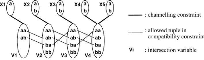
When the arity of the constraint being slid is not great, we can en-force GAC on SLIDEusing dynamic programming (DP) in a similar way to the DP-based propagators for the REGULARand STRETCH constraints [16, 13]. A much simpler method, however, which is just as efficient and effective as dynamic programming is to exploit a variation of the dual encoding into binary constraints [10] based on tuples of support. Such an encoding was proposed in [1] for a par-ticular sliding constraint. Here we show that this method is more general and can be used for arbitrary SLIDEconstraints. Using such an encoding, SLIDEcan be easily added to any constraint solver. We illustrate the intersection encoding by means of an example.

Consider again the AMONGSEQ example in which 2 of ev-ery 3 variables of X1. . . X5 should take the value a, where

X1 = a and X2, . . . , X5 ∈ {a, b}. We can encode this as

SLIDE(E, [X1, X2, X3, X4, X5]) where E(Xi, Xi+1, Xi+2) is an

instance of the AMONGconstraint that ensures two of its three vari-ables takea. If the sliding constraint has arity k, we introduce an

intersection variable for each subsequence of k − 1 variables of

SLIDE. The first intersection variable V1 has a domain containing

: intersection variable ab aa ba bb ab aa ba bb a X1 b a X2 b a X4 b a X5 b a X3 ab aa bb ba ab aa V2 V3 V4 V1 compatibility constraint : channelling constraint : allowed tuple in Vi

Figure 1. Intersection encoding

all tuples fromD(X1) × . . . × D(Xk−1). The jth intersection

vari-ableVjhas domain containingD(Xj) × . . . × D(Xj+k−2). And

so on untilVn−k+2. In our example in Fig 1, this givesD(V1) =

D(X1) × D(X2), . . . , D(V4) = D(X4) × D(X5). We then post

bi-nary compatibility constraints between consecutive intersection vari-ables. These constraints ensure that the two intersection variables assign(k − 1)-tuples that agree on the values of their k − 2

com-mon original variables (like constraints in the dual encoding). They also ensure that thek-tuple formed by the two (k − 1)-tuples

sat-isfies the corresponding instance of the slid constraint. For instance, in Fig 1, the binary constraint betweenV1 andV2 does not allow

the pairhab, aai because the second argument of ab for V1(valueb

forX2) is in conflict with the first argument ofaa for V2(valuea for

X2). That same constraint betweenV1andV2does not allow the pair

hab, bbi because the tuple abb is not allowed by E(X1, X2, X3).

Enforcing AC on such compatibility constraints prunesaa and bb

fromV2, ab and bb from V3, andba and bb from V4. Finally, we

post binary channelling constraints to link the tuples to the original variables. One such constraint for each original variable is sufficient. For example, we can have a channelling constraint betweenV4and

X4which ensures that the first argument of the tuple assigned toV4

equals the value assigned toX4. Enforcing AC on this channelling

constraint prunesb from the domain of X4. We could instead post a

channelling constraint betweenV3andX4ensuring that the second

argument inV3equalsX4. The AMONGSEQconstraint is now GAC. Theorem 3 Enforcing AC on the intersection encoding of SLIDE

achieves GAC inO(ndk_{) time and O(nd}k−1_{) space where k is the}

arity of the constraint to slide andd is the maximum domain size.

Proof: The constraint graph associated with the intersection encoding is a tree. Enforcing AC on this therefore achieves GAC. Enforcing AC on the channelling constraints then ensures that the domains of the original variables are pruned appropriately. As we introduce O(n) intersection variables, and each can contain O(dk−1_{) tuples, the intersection encoding requires O(nd}k−1₎

space. Enforcing AC on a compatibility constraint between two intersection variablesVi andVi+1 takesO(dk) time as each tuple

in the intersection variableVihas at mostd supports which are the

tuples ofVi+1that are equal toVion theirk − 2 common arguments.

Enforcing AC on O(n) such constraints therefore takes O(ndk₎

time. Finally, enforcing AC on each of the O(n) channelling

constraints takesO(dk−1_{) time as they are functional. Hence, the}

total time complexity isO(ndk_{). 2}

Arc consistency on the intersection encoding simulates pairwise consistency on the decomposition. It does this efficiently as inter-section variables represent in extension ’only’ the interinter-sections. This is sufficient because the constraint graph is acyclic. This encoding is also very easy to implement in any constraint solver. It has good

incremental properties. Only those constraints associated with a vari-able which changes need to wake up.

The intersection encoding of SLIDEjforj > 1 is less expensive

to build than forj = 1 as we need intersection variables for

subse-quences of less thank − 1 variables. For 1 ≤ j ≤ k/2, we introduce

intersection variables for subsequences of variables of lengthk − j

starting at indices1, j + 1, 2j + 1... whose domains contain (k −

j)-tuples of assignments. Compatibility and channelling constraints are defined as withj = 1. If j > k/2, two consecutive intersection

vari-ables (for two subsequences ofk − j variables) involve less than k

variables of the SLIDEj. The compatibility constraint between them

cannot thus ensure the satisfaction of the slid constraint. We therefore introduce intersection variables for subsequences of length ⌈k/2⌉

starting at indices1, j + 1, 2j + 1... and for subsequences of length ⌈k/2⌉ finishing at indices k, j + k, 2j + k... The compatibility

con-straint between two consecutive intersection variables representing the subsequence starting at indexpj + 1 and the subsequence

fin-ishing at indexpj + k ensures satisfaction of the (p + 1)th instance

of the slid constraint. The compatibility constraint between two con-secutive intersection variables representing subsequence finishing at indexpj + k and the subsequence starting at index (p + 1)j + 1

ensures the consistency of the arguments in the intersection of two instances of the slid constraint.

7

EXPERIMENTS

We now demonstrate the practical value of SLIDE. Due to space limits, we only report detailed results on a nurse scheduling prob-lem, and summarise the results on balanced incomplete block design generation and car sequencing problems. Experiments are performed with ILOG Solver 6.2 on a 2.8GHz Intel computer running Linux.

We consider a Nurse Scheduling Problem [9] in which we gener-ate a schedule of shift duties for a short-term planning period. There are three types of shifts (day, evening, and night). We ensure that (1) each nurse takes a day off or is assigned to an available shift; (2) each shift has a minimum required number of nurses; (3) each nurse’s work load is between specific lower and upper bounds; (4) each nurse works at most 5 consecutive days; (5) each nurse has at least 12 hours of break between two shifts; (6) the shift assigned to a nurse does not change more than once every three days. We con-struct four different models, all with variables indicating what type of shift, if any, each nurse is working on each day. We break symme-try between the nurses with lex concstraints. The constraints (1)-(3) are enforced using global cardinality constraints. Constraints (4), (5) and (6) form sequences of respectively 6-ary, binary and ternary con-straints. Since (4) is monotone, we simply post the decomposition in the first three models. This achieves GAC by Theorem 1. The mod-els differ in how (5) and (6) are propagated. Indecomp, they are decomposed into conjunction of slid constraints. Inamongseq, (5) is decomposed and (6) is enforced using the AMONGSEQconstraint of ILOG Solver (called IloSequence). The combination of (5) and (6) are enforced by SLIDEinslide. Finally, inslidec, we

use SLIDEfor the combination of (4), (5), and (6).

We test the models using the instances available at

http://www.projectmanagement.ugent.be/nsp.php in which nurses

have no maximum workload, but a set of preferences to optimise. We ignore these preferences and post a constraint bounding the maximum workload to at most 5 day shifts, 4 evening shifts and 2 night shifts per nurse and per week. Similarly, each nurse must have at least 2 rest days per week. We solve three samples of instances involving 25, 30 and 60 nurses to schedule over 28 days.

We use the same variable ordering for all models so that heuristic choices do not affect results. We schedule the days in chronological order and within each day we allocate a shift to every nurse in lexi-cographical order. Initial experiments show that this is more efficient than the minimum domain heuristic. However, it restricts the variety of domains passed to the propagators, and thus hinders any demon-stration of differences in pruning. We therefore also use a more ran-dom heuristic. We allocate within each day a shift to every nurse randomly with20% frequency and lexicographically otherwise.

#solved bts1 _time1 _bts2 _time2 25 nurses, 28 days (99 instances)

decomp 99 301 0.13 301 0.13

amongseq 99 301 0.19 301 0.19

slide 99 301 0.19 301 0.19

slidec 99 295 0.68 295 0.68

30 nurses, 28 days (99 instances)

decomp 68 7101 2.80 15185 5.29

amongseq 67 7101 4.31 7150 4.33

slide 70 3303 1.99 4319 2.53

slidec 75 1047 2.13 11014 10.02

60 nurses, 28 days (100 instances)

decomp 51 5999 4.38 5999 4.38

amongseq 51 5999 7.10 5999 7.10

slide 52 5300 5.61 8479 7.21

slidec 58 2157 7.52 4501 12.07

Table 1. Nurse scheduling with lexicographical variable ordering (1_on instances solved by all methods,2_{on instances solved by the method).}

#solved bts1 time1 bts2 time2 25 nurses, 28 days (99 instances)

decomp 86 35084 7.69 41892 10.06

amongseq 85 35401 14.43 35401 14.43

slide 97 1699 1.00 1547 0.92

slidec 97 457 0.58 438 0.56

30 nurses, 28 days (99 instances)

decomp 20 68834 11.94 69550 12.75

amongseq 20 68834 18.89 69550 19.83

slide 42 378 0.18 8770 7.29

slidec 43 365 0.95 12857 6.76

60 nurses, 28 days (100 instances)

decomp 3 122406 71.06 250427 142.90

amongseq 2 122406 119.40 122406 119.40

slide 27 562 0.65 2367 2.19

slidec 34 542 3.96 1368 6.38

Table 2. Nurse scheduling with random variable ordering (1_{on instances} solved by all methods,2_{on instances solved by the method).}

Tables 1 and 2 report the mean runtime and fails to solve the in-stances with 5 minutes cutoff. Between the first three models, the best results are due toslide. We solve more instances with slide, as well as explore a smaller tree. By developing a propagator for a generic constraint like SLIDE, we can increase pruning without hurting efficiency. Note that slide always performs better than

amongseq. A possible reason is that AMONGSEQcannot encode constraint (6) as directly as SLIDE. As in previous models, we need to channel into Boolean variables and post AMONGSEQ on them. This may not give as effective and efficient pruning. SLIDEthus of-fers both modelling and solving advantages over existing sequencing constraints. Note also thatslidecsolves additional instances in the

time limit. This is not suprising as the model slides the combination of the constraints (4), (5), and (6). Recall that the sliding constraint of (4) is 6-ary. It is pleasing to note that the intersection encoding performs well even in the presence of such a high arity constraint.

We also ran experiments on Balanced Incomplete Block Designs (BIBDs) and car sequencing. For BIBD, we use the model in [12] which contains LEX constraints. We propagate these either using the specialised algorithm of [12] or the SLIDEencoding. As both propagators maintain GAC, we only compare runtimes. Results on large instances show that the SLIDEmodel is as efficient as the LEX

model. For car sequencing, we test the scalability of SLIDEon large arity constraints and large domains using80 instances from CSPLib.

Unlike a model usingIloSequence, our SLIDEmodel does not combine reasoning about overall cardinality of a configuration with the sequence of AMONGconstraints. Hence, it is not as efficient:26

instances were solved with SLIDEwithin the five minute cutoff, com-pared to39 withIloSequence. However,9 of the instances solved

with SLIDEwere not solved byIloSequence. The memory over-head of the SLIDEpropagator was not excessive despite the slid con-straints having arity5 and domains of size 30. The SLIDEmodel used on average22Mb of space, compared to 5Mb forIloSequence.

8

RELATED WORK

Pesant introduced the REGULARconstraint, and gave a propagator based on dynamic programming to enforce GAC [16]. As we saw, the REGULARconstraint can be encoded using a simple SLIDE con-straint. In this simple case, the dynamic programming machinery of Pesant’s propagator is unnecessary as the decomposition into ternary constraints does not hinder propagation. We have found that SLIDE is as efficient as REGULARin practice [2]. Furthermore, our encod-ing introduces variables for representencod-ing the states. Access to the state variables may be useful (e.g. for expressing objective func-tions). Although an objective function can be represented with the COSTREGULAR constraint [11], this is limited to the sum of the variable-value assignment costs. Our encoding is more flexible, al-lowing different objective functions like the min function used in the example in Section 3.

Beldiceanu, Carlsson, Debruyne and Petit have proposed specify-ing global constraints by means of deterministic finite automata aug-mented with counters [6]. They automatically construct propagators for such automata by decomposing the specification into a sequence of signature and transition constraints. This gives an encoding sim-ilar to our SLIDEencoding of the REGULARconstraint. There are, however, a number of advantages of SLIDEover using an automaton. If the automaton uses counters, pairwise consistency is needed to guarantee GAC (and most constraint toolkits do not support pairwise consistency). We can encode such automata using a SLIDEwhere we introduce an additional sequence of variables for each counter. SLIDE thus provides a GAC propagator for such automata. Moreover, SLIDE has a better complexity than a brute-force pairwise consistency algo-rithm based on the dual encoding as it considers only the intersection variables, reducing the space complexity by a factor ofd.

Hellsten, Pesant and van Beek developed a GAC propagator for the STRETCHconstraint based on dynamic programming similar to that for the REGULARconstraint [13]. As we have shown, we can en-code the STRETCHconstraint and maintain GAC using SLIDE. Sev-eral propagators for the AMONGSEQare proposed and compared in [21, 3]. Among these propagators, those based on the REGULAR con-straint do the most pruning and are often fastest. Finally, Bartak has proposed a similar intersection encoding for propagating a sliding scheduling constraint [1] We have shown that this method is more general and can be used for arbitrary SLIDEconstraints.

9

CONCLUSIONS

We have studied the CARDPATHconstraint. This slides a constraint down a sequence of variables. We considered SLIDEa special case of CARDPATHin which the slid constraint holds at every position. We demonstrated that this special case can encode many global sequenc-ing constraints includsequenc-ing AMONGSEQ, CARDPATH, REGULARin a

simple way. SLIDEcan therefore serve as a “general-purpose” con-straint for decomposing a wide range of global concon-straints, facilitat-ing their integration into constraint toolkits. We proved that enforc-ing GAC on SLIDEis NP-hard in general. Nevertheless, we identi-fied several useful and common cases where it is polynomial. For instance, when the constraint being slid overlaps on just one vari-able or is monotone, decomposition does not hinder propagation. Dynamic programming or a variation of the dual encoding can be used to propagate SLIDEwhen the constraint being slid overlaps on more than one variable and is not monotone. Unlike the previous proposed propagator for CARDPATH, this achieves GAC. Our exper-iments demonstrated that using SLIDEto encode constraints can be as efficient and effective as specialised propagators. There are many directions for future work. One promising direction is to use binary decision diagrams to store the supports for the constraints being slid when they have many satisfying tuples. We believe this could im-prove the efficiency of our propagator in many cases.

REFERENCES

[1] R. Bartak, ‘Modelling resource transitions in constraint-based schedul-ing’, in Proc. of SOFSEM 2002: Theory and Practice of Informatics. (2002).

[2] C. Bessiere, E. Hebrard, B. Hnich, Z. Kiziltan, C.-G. Quimper and T. Walsh, ‘Reformulating global constraints: the SLIDE and REGU-LAR constraints’, in Proc. of SARA’07. (2007).

[3] S. Brand, N. Narodytska, C.-G. Quimper, P. Stuckey and T. Walsh, ‘En-codings of the SEQUENCE Constraint’, in Proc. of CP’07. (2007). [4] C. Beeri, R. Fagin, D. Maier, and M. Yannakakis, ‘On the desirability of

acyclic database schemes’, Journal of the ACM, 30, 479–513, (1983). [5] N. Beldiceanu and M. Carlsson, ‘Revisiting the cardinality operator and

introducing cardinality-path constraint family’, in Proc. of ICLP’01. (2001).

[6] N. Beldiceanu, M. Carlsson, R. Debruyne, and T. Petit, ‘Reformulation of global constraints based on constraints checkers’, Constraints, 10(4), 339–362, (2005).

[7] N. Beldiceanu, M. Carlsson, and J-X. Rampon, ‘Global constraints cat-alog’, Technical report, SICS, (2005).

[8] N. Beldiceanu and E. Contejean, ‘Introducing global constraints in CHIP’, Mathl. Comput. Modelling, 20(12), 97–123, (1994).

[9] E.K. Burke, P.D. Causmaecker, G.V. Berghe and H.V. Landeghem, ‘The state of the art of nurse rostering’, Mathl. Journal of Scheduling, 7(6), 441–499, (2004).

[10] R. Dechter and J. Pearl, ‘Tree clustering for constraint networks’,

Arti-ficial Intelligence, 38, 353–366, (1989).

[11] S. Demassey, G. Pesant, and L.-M. Rousseau, ‘A cost-regular based hybrid column generation approach’, Constraints, 11(4), 315–333, (2006).

[12] A. Frisch, B. Hnich, Z. Kiziltan, I. Miguel, and T. Walsh, ‘Global con-straints for lexicographic orderings’, in Proc. of CP’02. (2002). [13] L. Hellsten, G. Pesant, and P. van Beek, ‘A domain consistency

algo-rithm for the stretch constraint’, in Proc. of CP’04. (2004).

[14] Y.C. Law and J.H.M. Lee, ‘Global constraints for integer and set value precedence’, in Proc. of CP’04. (2004).

[15] M. Maher, ‘Analysis of a global contiguity constraint’, in Proc. of the

CP’02 Workshop on Rule Based Constraint Reasoning and Program-ming, (2002).

[16] G. Pesant, ‘A regular language membership constraint for finite se-quences of variables’, in Proc. of CP’04. (2004).

[17] P. Refalo, ‘Linear formulation of constraint programming models and hybrid solvers’, in Proc. of CP’00. (2000).

[18] J-C. R´egin, ‘A filtering algorithm for constraints of difference in CSPs’, in Proc. of AAAI’94. (1994).

[19] P. Van Hentenryck and J.-P. Carillon, ‘Generality versus specificity: An experience with AI and OR techniques’, in Proc. of AAAI’88. (1988). [20] W-J. van Hoeve, G. Pesant, and L-M. Rousseau, ‘On global warming :

Flow-based soft global constaints’, Journal of Heuristics, 12(4-5), 347– 373, (2006).

[21] W-J. van Hoeve, G. Pesant, L-M. Rousseau, and A. Sabharwal, ’Revis-iting the sequence constraint’ in Proc. of CP’06. (2006).