Experimental investigation of the variability of concrete durability properties

HAL Id: hal-00845982

https://hal.archives-ouvertes.fr/hal-00845982

Submitted on 18 Jul 2013

HAL is a multi-disciplinary open access archive for the deposit and dissemination of sci-entific research documents, whether they are pub-lished or not. The documents may come from teaching and research institutions in France or

L’archive ouverte pluridisciplinaire HAL, est destinée au dépôt et à la diffusion de documents scientifiques de niveau recherche, publiés ou non, émanant des établissements d’enseignement et de recherche français ou étrangers, des laboratoires

Experimental investigation of the variability of concrete

durability properties

Abdelkarim Aît-Mokhtar, Jean Michel Torrenti, Farid Benboudjema, Bruno

Capra, Myriam Carcasses, Jean-Baptiste Colliat, François Cussigh, Thomas

de Larrard, Jf Lataste, Stéphane Poyet, et al.

To cite this version:

Abdelkarim Aît-Mokhtar, Jean Michel Torrenti, Farid Benboudjema, Bruno Capra, Myriam Carcasses, et al.. Experimental investigation of the variability of concrete durability properties. Cement and Concrete Research, Elsevier, 2013, 45, pp. 21-36. �10.1016/j.cemconres.2012.11.002�. �hal-00845982�

Experimental investigation of the variability of concrete durability

1

properties.

2

A. Aït-Mokhtara, R. Belarbia, F. Benboudjemab, N. Burlionc, B. Caprad, M. Carcassèse, J-B. Colliatb, F. Cussighf, F. Debye, F. Jacquemotg, T. de 3

Larrardb, J-F. Latasteh, P. Le Bescopi, M. Pierrei, S. Poyeti, P. Rougeaug, T. Rougelotc, A. Selliere, J. Séménadissef, J-M. Torrentij, A. Trabelsia, Ph. 4

Turcrya, H. Yanez-Godoyd 5

6

a

Université de La Rochelle, LaSIE FRE-CNRS 3474, Avenue Michel Crépeau, F-17042 La Rochelle Cedex 1, France. 7

b

LMT/ENS Cachan/CNRS UMR 8535/UPMC/PRES UniverSud Paris, 61 Avenue du Président Wilson, F-94235 Cachan, France. 8

c

Laboratoire de Mécanique de Lille, Boulevard Paul Langevin, Cité Scientifique, F-59655 Villeneuve d’Ascq Cedex, France. 9

d

Oxand, 49 Avenue Franklin Roosevelt, F-77210 Avon / Fontainebleau, France. 10

e

Université de Toulouse, UPS, INSA, LMDC (Laboratoire Matériaux et Durabilité des Constructions), 135 Avenue de Rangueil, F-31077 Toulouse 11

Cedex 4, France. 12

f

Vinci Construction France, Direction des Ressources Techniques et du Développement Durable, 61 Avenue Jules Quentin, F-92730 Nanterre 13

Cedex, France. 14

g

CERIB, Rue des Longs Réages, BP 30059, F-28231 Epernon, France. 15

h

Université Bordeaux 1, I2M CNRS UMR5295, Avenue des facultés, Bât. B18, F-33400 Talence, France. 16

i

CEA, DEN, DPC, SECR, Laboratoire d’Etude du Comportement des Bétons et des Argiles, F-91191 Gif sur Yvette Cedex, France. 17

j

Université Paris-Est, IFSTTAR, 58 Boulevard Lefebvre, F-75732 Paris Cedex 15, France. 18

19

Abstract

20

One of the main objectives of the APPLET project was to quantify the variability of concrete properties to allow for a probabilistic 21

performance-based approach regarding the service lifetime prediction of concrete structures. The characterization of concrete variability was the 22

subject of an experimental program which included a significant number of tests allowing the characterization of durability indicators or 23

performance tests. Two construction sites were selected from which concrete specimens were periodically taken and tested by the different 24

project partners. The obtained results (mechanical behavior, chloride migration, accelerated carbonation, gas permeability, desorption 25

isotherms, porosity) are discussed and a statistical analysis was performed to characterize these results through appropriate probability density 26

functions. 27

28

Keywords: concrete – durability indicators – performance tests – variability. 29

30

1. Introduction / context

31

The prediction of the service lifetime of new as well as existing concrete structures is a global challenge. Mathematical models are needed to 32

assess to allow for a reliable prediction of the behavior of these structures during their lifetime. The French APPLET project was undertaken in 33

order to improve these models and improve their robustness [1]. The main objectives of this project were to quantify the various sources of 34

variability (material and structure) and to take these into account in probabilistic approaches, to include and to understand in a better manner 35

the corrosion process, in particular by studying its influence on the steel behavior, to integrate knowledge assets on the evolution of concrete 36

and steel properties in order to include interface models between the two materials, and propose relevant numerical models, to have robust 37

predictive models to model the long term behavior of degraded structural elements, and to integrate the data obtained from monitoring or 38

inspection. 39

Within this project, working group 1 (WG1) has taken into consideration the variability of the material properties for a probabilistic 40

concretes was the subject of an experimental program with a significant number of tests allowing the characterization of indicators of durability 42

or tests related to durability. After the presentation of the construction sites where the concrete specimens were produced in industrial 43

conditions (using ready mix plants), the obtained results of the different tests (mechanical behavior, chloride migration, carbonation, 44

permeability, desorption isotherms, porosity) are discussed and probability density functions are associated to these results. 45

2. Case studies

46

The objective of the project was the characterization of the variability of concretes produced in industrial conditions. This variability is due to 47

the natural variability of the constituents of concrete, to errors in constituents weighing, to quality of vibration and compaction, to the initial 48

concrete temperature, to environmental conditions, etc. For the supply of specimens, the project takes advantage from the support of Vinci 49

Construction France. Two construction sites where two concretes were prepared continuously during at least 12 months regularly provided 50

specimens to the various participants for the execution of their tests: works for the south tunnel in Highway A86 (construction site A1) and for a 51

viaduct near Compiègne (north of Paris - construction site A2). 52

The first specimen denoted A1-1 was cast on 6th March 2007 at the tunnel construction site (Table 1), and then specimens were prepared and 53

provided with a frequency of about one week. The concrete was a C50/60 (characteristic compressive strength at 28 days) containing Portland 54

cement (CEM I) and fly-ashes used for the construction of the slab separating the two lanes from the tunnel of Highway A86 (Table 1). The 55

concrete was prepared using the concrete plant on site by the site workers. Forty batches were made on this first construction site. The last 56

specimen was cast on the 31st March 2008. In fact, for each date, 15 specimens (cylinders with a diameter of 113 mm and a height of 226 mm; 57

note that these shape and dimensions are accepted by the European standards EN 12390 and the French version of the ENV 206-1) were 58

produced and dispatched to the 7 laboratories participating in the project. 59

At the second construction site a concrete C40/50 was produced containing CEM III cement which was used for the construction of the 60

supports (foundations, piles) of the viaduct of Compiegne (Table 1). The first specimens (A2-1) were produced the 6th of November 2007 at the 61

viaduct construction site. The concrete was also prepared by the site workers using a ready mix concrete. However, from batch A2-21 on, due to 62

work constraints another composition corresponding to the same concrete quality was used to improve the concrete workability (denoted A2/2). 63

Finally, forty batches were produced, each composed of 14 specimens dispatched to the 7 laboratories involved. The last batch was produced the 64

21st of January 2009. 65

66

Table 1 - Concrete mixes (per m3 of concrete). 67

Site A1 A2/1 A2/2

Cement C CEM I 52.5 - 350 kg CEM III/A 52.5L LH - 355 kg

Additions A Fly ash - 80 kg Calcareous filler - 50 kg

Water W 177 L 176 L 193 L

W/C 0.51 0.50 0.54

68

It must be added here that all the specimens used in this project were prepared on the two sites by the site workers simultaneously to the 69

fabrication of the slabs and supports of the construction sites A1 and A2, respectively. In the authors’ mind, the concrete specimens are then 70

made of “realcrete” and are believed to be more or less representative of the materials that can be encountered within the considered 71

corresponding structural elements because the impact of some worksite features (for instance presence of reinforcement, structural element 73

dimensions and height of chute) could not be reproduced using small specimens. 74

75

3. Experimental results

76

3.1. Compressive and tensile strengths

77

This part of the research aims at proposing a characterization of the mechanical behavior of each studied batch by standard tests to 78

determine the tensile strength (by a splitting test), and also the compressive strength and Young's modulus (through a compression test). The 79

tests were performed at LMT of the Ecole Normale Supérieure de Cachan. For each batch, a cylindrical 113×226 mm specimen is devoted to 80

compression test, while the splitting test is performed on a cylindrical specimen of 113 mm in diameter and 170 mm in height (the upper part of 81

the specimen is used for porosity and pulse velocity measurements). 82

For the compression test, the specimen is mechanically grinded before being placed in press. The specimen is equipped with an extensometer 83

(three LVDTs positioned at 120 degrees attached to a metal ring, which is fixed on the concrete specimen by set screws) to measure the 84

longitudinal strain of the specimen during the loading phase assumed to be elastic, between 5 and 30% of the failure load in compression. Three 85

cycles of loading and unloading are performed in the elastic behavior region of the concrete, with a loading rate of 5 kN/s (the rate is the same 86

for unloading). Young’s modulus is determined by linear regression on five points placed on the curve corresponding to the third unloading, 87

according to the protocol proposed by [2]. Then, after removing the extensometer, the specimen is loaded until failure. 88

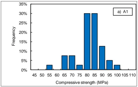
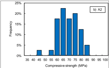
Table 2 and Figure 1 to Figure 3 present an overview of the results derived from the mechanical tests (mean value, standard deviation, 89

coefficient of variation1 and number of specimens tested). It can be observed that the compressive strength is much higher than expected 90

according to the compressive strength class and to the achieved values of compressive strength at 28 days (measured on site). This is due to the 91

fact that the specimens were tested after one year of curing in saturated lime water resulting in a higher hydration degree which improves the 92

strength. The magnitude of the coefficient of variation is similar for the compressive and tensile strengths: around 10%. However, the variability 93

observed for Young's modulus is significantly lower (between 5 and 7%). 94 95 0% 5% 10% 15% 20% 25% 30% 35% 45 50 55 60 65 70 75 80 85 90 95 100 105 110 F re q u e n c y

Compressive strength (MPa)

0% 5% 10% 15% 20% 25% 35 40 45 50 55 60 65 70 75 80 85 90 95 100 F re q u e n c y

Compressive strength (MPa)

b) A2

Figure 1 – Distribution of the compressive strength measured in laboratory (LMT) after 1 year curing. 96 97 0% 5% 10% 15% 20% 25% 30% 35% 2.5 3.0 3.5 4.0 4.5 5.0 5.5 6.0 6.5 7.0 7.5 F re q u e n c y

Tensile strength (MPa)

0% 5% 10% 15% 20% 25% 30% 35% 40% 45% 2.5 3.0 3.5 4.0 4.5 5.0 5.5 6.0 6.5 7.0 F re q u e n c y

Tensile strength (MPa)

b) A2

Figure 2 – Distribution of the tensile strength measured in laboratory (LMT) after 1 year curing. 98 99 0% 5% 10% 15% 20% 25% 30% 37 39 41 43 45 47 49 51 53 55 F re q u e n c y

Elastic modulus (GPa)

0% 5% 10% 15% 20% 25% 30% 35% 31 33 35 37 39 41 43 45 47 49 F re q u e n c y

Elastic modulus (GPa)

b) A2

Figure 3 – Distribution of the elastic modulus measured in laboratory (LMT) after 1 year curing. 100

101

Table 2 - Mechanical tests for 3 concrete mix designs: mean values, coefficient of variation and number of specimens tested for the 102

compressive (fc) and tensile (ft) strengths and Young’s modulus (E).

103

Site Number fc [MPa] ft [MPa] E [GPa]

Mean COV (%) Mean COV (%) Mean COV (%)

A1 40 83.8 10.5 4.9 13.2 46.8 6.2

A2-1 20 75.6 11.3 5.1 9.7 40.8 7.0

A2-2 20 68.2 9.0 4.8 9.3 40.8 5.4

104

The magnitude of the coefficient of variation is similar to what Mirza et al. [3] and Chmielewski & Konokpa [4] have observed for the 105

variability of the compressive strength for “monitored” concrete (produced with great care), but their strengths were lower than those of the 106

APPLET project materials. For high-performance concrete, having a compressive strength that is similar to that observed within this study, the 107

variability observed by Torrenti [5] and Cussigh et al. [6] is approximately two times lower than it is here. 108

Simultaneously, the compressive strengths were also measured on site at age of 28 days. The specimens used were fabricated and kept in the 109

same way as the ones that were sent to the involved laboratories. The tests were performed by Vinci Construction France using the same test 110

conditions as detailed above. 116 specimens were tested for the construction site A1 and 114 for the construction site A2 (that is to say three 111

different specimens from the same batch were tested at the same time except for some batches for which only two specimens were used). The 112

results obtained for the variability are very similar to the previous ones (Table 3 and Figure 4). 113 114 0% 5% 10% 15% 20% 25% 30% 37 40 43 46 49 52 55 58 61 64 67 70 73 76 F re q u e n c y

0% 5% 10% 15% 20% 25% 34 37 40 43 46 49 52 55 58 61 64 67 70 73 76 79 F re q u e n c y

Compressive strength at 28 days (MPa) b) A2 site

Figure 4 – Distribution of the compressive strength (at 28 days) measured on site by Vinci Construction France. 115

116

Table 3 – Compressive strength measured on site by Vinci Construction France: number of tests (Nb), mean value and coefficient of variation 117 (COV). 118 Site Nb fc [MPa] Mean COV (%) A1 40 58.2 7.3% A2-1 20 57.8 11.1% A2-2 20 52.6 11.1% 119

3.2. Chloride migration

Non-steady state migration tests have been performed at LMDC (Toulouse University) in order to measure the chloride migration coefficient. 121

For the two selected construction sites, an overview of the results will be presented in the following sections. 122

The principle of the test method is described in the standard NT Build 492 [7]. The specimens were kept in water until the start of the test. 123

The experiments were performed for similar maturity of each specimen in the same series in order not to introduce on the results the effect of 124

the evolution of the concrete. Due to the equipments and the constraints of organizing this extensive significant experimental campaign, 125

experiments were launched at an age of 3 months for the A1 series and an age of 12 months for A2. Furthermore, it should be noted that logistic 126

problems were encountered: some deadlines were not respected and in these situations, the test was not conducted. Consequently, on the 40 127

initially planned, only 30 specimens from the A1 series and 31 from the A2 series were tested. 128

At the date of test, the specimen is then prepared. Once out of the storage room, specimens are cut to retain only a cylinder Ø113mm of 129

50mm height. The test specimen is taken from the central part of the specimen by cutting the top 50 millimeters from the free surface. The 130

concrete surface closest to the latter is then exposed to chlorides (Figure 5). 131 132 Free surface 50 mm 110 mm 50 mm Exposed surface 133

Figure 5 – Specimen preparation for the chloride migration test. 134

135

The specimen is then introduced in a rubber sleeve, and after clamping, sealing is ensured by a silicone sealant line. At first a leakage test is 136

which receives the sleeve) corresponds to the upstream compartment. The upper compartment contains the catholyte solution, i.e. a solution of 138

10% sodium chloride by mass (about 110 grams per liter) whereas the downstream compartment is filled with the anolyte solution, 0.3 M 139

sodium hydroxide. These solutions are stored in the conditioned test room at 20 °C. In each compartment an electrode is immersed, which is 140

externally connected through a voltage source so that the cathode, immersed in the chloride solution, is connected to the negative pole and the 141

anode, placed in the extending part of the sleeve, is connected to the positive pole. An initial voltage of 30 V is applied to the specimen. This 142

voltage is then adjusted to achieve a duration test of 24 hours depending on the magnitude of the current flowing through the cell as a result of 143

the initial voltage of 30 V. The correction is proposed in the standard NT Build 492 [7]. For A1 specimens, for the entire series the voltage used for 144

the test is 35 V whereas 50 V is applied for the entire A2 series. 145

After 24 hours, the specimen is removed to be split in two pieces. Silver nitrate AgNO3 is then sprayed onto the freshly fractured concrete

146

surface. The white precipitate of silver chloride appears after ten minutes revealing the achieved chloride penetration front. At the concrete 147

surface where chlorides are not present silver nitrate will not precipitate but will quickly oxidize and then turn black after a few hours. The 148

chloride penetration depth in concrete xd is then measured using a slide caliper using an interval of 10 mm to obtain 7 measured depths. To avoid

149

edge effects, a distance of 10 mm is discarded at each edge. Moreover, if the front ahead of a measuring point is obviously blocked by an 150

aggregate particle, then the associated measured depth is rejected. Then the migration coefficient Dnssm (non steady state migration) (m²/s) is

151

calculated using the following formula: 152 153













155

where U is the magnitude of the applied voltage (V), T the temperature in the anolyte solution (°C), L the thickness of the specimen (mm), xd the

156

average value of the chloride penetration depth (mm) and t the test duration (h). All the results are shown in Figure 6 which shows the migration 157

coefficient obtained for the specimens from the A1 series. 158

The measured values vary around a mean value of 4.12×10-12 m²/s. The potential resistance against chloride ingress is then high. This can be 159

easily explained by the formulation of this C50/60 concrete where fly ash was used, which is known to significantly reduce the diffusion 160

coefficient [8]. The minimum value observed is 3.11×10-12 m²/s and the maximum amounts to 5.59×10-12 m²/s which corresponds to a ratio of 161

1.8. The difference may seem relevant but basically corresponds to a divergence in concrete porosity of about 1.5% if the migration coefficients 162

are estimated from basic models [9]. The standard deviation is equal 0.53×10-12 m²/s; this corresponds to a coefficient of variation of 12.4% 163

(Table 4). 164

0% 5% 10% 15% 20% 25% 30% 35% 40% 2.61 3.11 3.61 4.10 4.60 5.10 5.59 6.09 F re q u e n c y Dnssm(x10-12m2/s) 166

Figure 6 – Histogram of the migration coefficient from the A1 series. 167

168

For the A2 series the experiments could not be conducted on specimens A2-12 to A2-20. The migration experiments have been resumed from 169

A2-21, which corresponds to the modified mix design of the A2 series. The mean migration coefficients determined for the complete A2 series is 170

2.53×10-12 m²/s with a standard deviation of 0.55×10-12 m2/s corresponding to a coefficient of variation of 21.9%. Compared to the concrete of 171

the A1 series, the resistance of this concrete against chloride ingress is significantly higher. The average value is even smaller however for this A2 172

series concrete specimens were tested at a later age, i.e. one year instead of three months for A1. The second concrete (A2) would certainly 173

achieve more modest results at a younger age because of the slow hydration kinetics for this type of cement containing blast furnace slag. 174

In the same way as for the A1 series, all these results may be grouped in a histogram. In contrast, as A2 series contains two mix design 175

formulations, the results must be treated in two subsets. In addition, the first formulation contains only 11 results, whereas the histogram of the 176

second formulation of this A2 reflects 20 experimental values (Figure 7). The mean migration coefficient of the second formulation of the A2 177

series amounts to 2.45×10-12 m²/s with a standard deviation of 0.47×10-12 m²/s, which corresponds to a coefficient of variation of 19.4% (Table 4). 178

It should be noted that the mean value and coefficient of variation are lower for the second formulation of the A2 series. This corresponds to 179

observations on site (higher variability of the workability for A2-1) that has decided the Vinci Company to modify the formulation. 180 181 0% 5% 10% 15% 20% 25% 30% 35% 40% 1.38 1.81 2.24 2.68 3.11 3.54 3.97 F re q u e n c y Dnssm(x10-12m2/s) 182

Figure 7 – Histogram of the migration coefficient for the A2-2 series. 183

184

The variability is higher than for the A1 series since the coefficient of variation increases from 12.4% to 19.5% (and even larger if A2-1 185

consider is considered). 186

Table 4 – Migration coefficient: number of tests (Nb), mean value and coefficient of variation (COV). 188 Site Nb Dnssm [10 -12 m2/s] Mean COV (%) A1 30 2.53 12.4% A2-1 11 2.67 25.4% A2-2 20 2.45 19.4% 189

3.3. Water Vapour desorption isotherm

190

Water vapour sorption-desorption isotherms tests were performed at the LaSIE at La Rochelle University [10]. This test characterizes water 191

content in a porous medium as a function of relative humidity at equilibrium state. It expresses the relationship between the water content of 192

the material and relative humidity (RH) of the surrounding air for different moisture conditions defined by a RH ranging from 0 to 100%. 193

The method undertaken in this study for the assessment of desorption isotherms is based on gravimetric measurements [11, 12]. Specimens 194

were placed in containers under isothermal condition (23 ± 1°C). The relative humidity of the ambient air is regulated using saturated salt 195

solutions. For each of the following moisture stages: RH = 90.4%, 75.5%, 53.5%, 33%, 12% and 3%, a regular monitoring of mass specimen in time 196

was performed until equilibrium was obtained characterized by a negligible variation of relative mass. The weighing of specimens was performed 197

inside the container as to result into the least disturbance of the relative humidity during measurements. The equilibrium is assumed to be 198

achieved if the hereafter criterion is satisfied: 199 200 % 005 . 0 ) 24 ( ) 24 ( ) ( _    h t m h t m t m (2) 201 202

where m(t) is the mass measured at the moment t and m(t + 24h) is the measured mass 24 hours later. 203

The test started with specimens which were initially saturated. To achieve the saturation, the adopted procedure consists in storing the 204

cylindrical specimens Ø113×226mm under water one day after mixing during at least 4 months. Besides, this procedure promotes a high degree 205

of hydration of cement. At the age of 3 months, these specimens were sawn in discs of 113 mm diameter and 5 ± 0.5 mm thickness. In these 206

discs a 4 mm diameter hole was drilled allowing mass measurements to be made inside the controlled RH environment with an accuracy of 0.001 207

g. At construction site A1, 3 specimens 113×226mm per batch were used and in the case of construction site A2, only the first concrete 208

composition (i.e. A2-1) was studied with 3 specimens per batch and overall, 180 specimens were studied. 209

Figure 8 shows the isothermal desorption curves for compositions A1 and A2-1. The water contents at equilibrium for the different RH levels 210

were calculated on the basis of dry mass measured at the equilibrium state for 3% RH. The so-obtained desorption isotherms belong to type IV 211

according to the IUPAC classification [13]. These are characterized by two inflections which are often observed for such a material [12]. 212

Desorption is thus multi-molecular with capillary condensation over a broad interval, which highlights a pore size distribution with several modes 213

(i.e. with several inflections points. For a given RH, concrete mixture A2-1 has higher average water content, especially for RH levels above 50%. 214

This is rather consistent with the mix proportions since mixture A2-1 has higher initial water content than mixture A1. 215

0 1 2 3 4 5 6 0 20 40 60 80 100 W a te r c o n te n t (% ) Relative humidity (%) A1 A2-1 217

Figure 8 – Average isothermal desorption curves for mixtures A1 and A2-1. 218

219

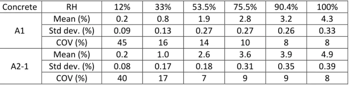
Table 5 gives the average water content values calculated at equilibrium with the different tested humidity environments and the 220

corresponding standard deviations and coefficients of variation. The coefficient of variation for 3 specimens from a single batch is approximately 221

equal to 10% for RH levels between 100 and 33% and equal to 20% for RH = 12%. The coefficients of variation determined over the complete 222

construction period (given in Table 5) are higher than the coefficients of variation for a single batch. The observed dispersion is not only due to 223

the randomness of test measurements, but also due to variability of material properties under site conditions [14]. It should be recalled that 224

mixtures were made in real ready-mix concrete plants. 225

Table 5 – Water vapour desorption isotherm: average values, standard deviations (Std dev.) and coefficients of variations (COV) of water 227

contents at equilibrium (throughout the construction period). 228 Concrete RH 12% 33% 53.5% 75.5% 90.4% 100% A1 Mean (%) 0.2 0.8 1.9 2.8 3.2 4.3 Std dev. (%) 0.09 0.13 0.27 0.27 0.26 0.33 COV (%) 45 16 14 10 8 8 A2-1 Mean (%) 0.2 1.0 2.6 3.6 3.9 4.9 Std dev. (%) 0.08 0.17 0.18 0.31 0.35 0.39 COV (%) 40 17 7 9 9 8 229

As shown in Figure 9, the statistical distributions of the water contents at equilibrium can be adequately modeled by normal probability 230

density functions. The parameter values of the normal probability density functions determined through regression analysis are given in Table 5. 231

232

234

3.4. Carbonation

235

The carbonation tests were performed at the CERIB and at the LaSIE (University of La Rochelle). For more details, the reader is referred to 236

[15]. From each construction site (A1 and A2), cylindrical specimens, 113mm in diameter and 226mm in height were sampled from different 237

batches. On site A1, 1 specimen per batch was sampled from the last 10 batches. On site A2, 3 specimens per batch were taken from 40 238

subsequent batches. After water curing during at least 28 days, each specimen was sawn at mid-height in order to obtain a disc, 113mm in 239

diameter and 50mm in height. 240

The protocol of the accelerated carbonation test is described in the French Standard XP P18-458. Concrete discs were first oven-dried at 45 ± 241

5°C during 14 days. After this treatment, the lateral side of the disks was covered by adhesive aluminum in order to ensure an axial CO2 diffusion

242

during the carbonation test. The discs were then placed in a chamber containing 50 ± 5% CO2 at 20 ± 2°C and 65% RH. After 28 days in this

243

environment, the concrete discs were split into two parts. A pH indicator solution, i.e. phenolphthalein, was sprayed on the obtained cross 244

sections in order to determine carbonation depth. The reported carbonation depth is the mean value of 24 measured depths per disc. 245

Table 6 gives an overview of the results of the accelerated carbonation tests. The average carbonation depth of A1 concrete is less than that 246

of A2 concretes. This can be attributed to the difference in binder type used in the concrete mixtures: slag substitution is known to enhance 247

carbonation [16, 17]. A significant difference can also be observed between the two mixtures from construction site A2. This difference might be 248

explained by a higher connectivity of the porous structure induced by the air-entraining effect of the plasticizer used for the second mixture A2-249

2. 250

The variability of the results is rather high. Figure 10 shows the statistical distribution of the carbonation depth in the case of construction site 251

A2. The distribution can be reasonably described by a normal probability density function (cf. §4.2). 252

253

Table 6 – Mean value, standard deviation and coefficient of variation of the carbonated depth. 254

Carbonation depth A1 A2-1 A2-2 A2

Mean value (mm) 4.3 7.6 12.6 10.1 Standard deviation (mm) 1.6 2.6 1.5 3.3 COV 37% 35% 12% 33% 255 0% 5% 10% 15% 20% 25% 30% F re q u e n c y Carbonation depth (mm) A2-1 A2-2 256

Figure 10 - Statistical distribution of the accelerated carbonation depths throughout the complete construction period (site A2). 257

3.5. Electrical resistivity

259

The electrical resistivity of concrete is generally a parameter measured on concrete structures to assess the probability of reinforcement 260

corrosion. However, because of its dependence on the porosity of the material [18], developments have been made for the assessment of 261

concrete transfer properties [19-21]. It appears increasingly as a durability indicator [18, 22]. 262

The investigations done within the APPLET program, aim at assessing the reliability of resistivity measurements for concretes properties, by 263

performing tests on 113×226mm cylindrical specimens using the resistivity cell technique in the laboratory. It consists in introducing an electrical 264

current of known magnitude in a concrete specimen and measuring the potential difference thus generated between two sensors on the 265

opposite specimen faces. Preliminary investigations have been done to study the influence of conditioning parameters on electrical resistivity 266

measurements. Finally, a light process has been defined to store specimens before resistivity measurement in the laboratory [23]. 267

The measurements have been performed at I2M in University Bordeaux1 (specimens having an age of 3 months, after continuous submersion 268

in water) and at LMT (specimens of 1 year , after continuous submersion in a saturated lime solution), according to a protocol defined to 269

distinguish different levels of variability [23]. The repeatability and reproducibility of laboratory measurement have been evaluated for each 270

specimen; the variability of the material within a batch (2 batches consisting of 20 specimens each are studied), and the variability of the material 271

during a year of casting (2 formulations studied from 40 specimens of test) are determined. 272

It is observed (Figure 11) that concrete A1 presents different ranges according to the laboratory: between 111 and 236 Ωm for 90 days old 273

concrete, and between 282 and 431 Ωm for 1 year-old concrete. This difference can essentially be attributed to the ageing, as was already 274

observed on concretes containing fly ash [24]. 275

276 0% 5% 10% 15% 20% 25% 30% 35% 40% F re q u e n c y Resistivity (Ω·m)

I2M (Univ. Bordeaux) LMT (ENS Cachan)

a) A1

277

Figure 11 – Resistivity distribution for concrete A1 (the specimens used at I2M were 90 days old whereas the age was 1 year at LMT). 278

0% 5% 10% 15% 20% 25% 30% 35% 40% F re q u e n c y Resistivity (Ω·m)

I2M (Univ. Bordeaux) LMT (ENS Cachan)

b) A2

280

Figure 12 – Resistivity distribution for concrete A2 (the specimens used at I2M were 90 days old whereas the age was 1 year at LMT). 281

282

Concrete A2 (Figure 12) does not present this difference despite the age difference and although the cement contains a significant amount of 283

slag. It is noted that both databases express a similar behavior even if measurements on 1 year old concrete show an expected light increase in 284

resistivity. However, for the distribution tail (towards the high resistivity values) the measured values range from 266 to 570 Ωm at an age of 90 285

days, and from 324 to 898 Ωm at an age of 1 year. These results show the difficulty to compare concretes using their resistivity values. Electrical 286

resistivity is a parameter which is very much influenced by the conditions during measurements (saturation degree of the specimen, 287

temperature, the nature of the saturation fluid). An overview of the variability assessment for both concretes is given in Table 7. 288

Table 7 – Electrical resistivity (Ωm): variability observed in laboratory. 290

Organism/Laboratory I2M LMT I2M LMT

Concrete A1 A1 A2 A2

Device used Resistivity cell Resistivity cell Resistivity cell Resistivity cell

Mean value 166.8 352.5 391.2 461.7

Mean repeatability r 0.005 - 0.007 -

Mean reproducibility R 0.015 0.006 0.012 0.007

Variability within a batch * Vb 0.023 0.076 0.036 0.035

Variability between batches VB 0.176 0.114 0.182 0.296

Age at measurements 90 days 1 year 90 days 1 year

* 590 days * at each term * 436 days * at each term

291

Variability linked to measurements is the repeatability (which characterizes the equipment), and the reproducibility (which also estimates the 292

noise due to the protocol). Whatever the concrete and laboratory are, it is concluded that these variabilities are good. They are indeed less than 293

2 % and underline that in laboratory the measurement results are accurate. The variability within a batch (Vb) is generally less than 5 % (except 294

for one year old concrete A1 which remains however less than 8 %). The variability between batches (VB) is determined to be less than 20 % 295

(except for the one year old concrete A2 which reaches 29.6 %, but this can be explained by the modification of the mix design during the 296

construction period). 297

Whatever the laboratory or the set of specimens considered, the variability is always ranked consistently: r <R <Vb <VB. The values of r and R 298

being low, variability Vb and VB are therefore only representative of the material variability. So, it is surprising to observe relatively large range, 299

for materials the engineer considers to be homogeneous and identical. These measurements show: (1) within a batch there are significant 300

differences between specimens; (2) for a single concrete cast regularly during one year, variability is less than 20%. 301

The differences observed between laboratories emphasize the importance of measurement conditions. Only measurements performed under 302

controlled conditions, regardless of the type of the specimen, should be considered. Any change in the conditioning (for instance temperature, 303

saturation or age) influences the resistivity values measured. 304

Resistivity measurements have also been done on a wall on site, made of A1 concrete, at an age of 28 days. On site value of reproducibility is 305

slightly higher than for the laboratory measurements (4.8%). 306

These results illustrate that the conditions of on-site measurements are less controlled. Even though this study is not sufficient to link the 307

variability of the concrete specimens to the concrete structural elements, it is however observed that on-site measurement and laboratory 308

techniques are consistent [23]. 309 310

3.6. Porosity

For the A1 construction site, specimens are denoted A1-x where x is the batch number (from 1 to 40). For the A2 construction site, as 2 313

different concrete mixes were studied (20 weeks for the first mix, then 20 weeks for the second), the specimens are denoted A2-y-x, where y is 314

the mix number (1 or 2) and x the batch number (specimen numbers range from A2-1-1 to A2-1-20, then A2-2-21 to A2-2-40). The determination 315

of porosity is studied through cylindrical specimens (diameter: 113 mm – height: about 50 mm) sawn from the bottom part of the bigger 316

cylindrical moulded specimens. This study was performed at the LMT. In particular, these tests aimed at analyzing the variability with respect to 317

the batch number (one batch per week); that is to say the ‘temporal variability’ of a given concrete. 318

Secondly, the variability of porosity inside a given concrete batch is also studied. Additional cylindrical moulded specimens of batch A1-13 and 319

A2-1-1 are cast. The porosity is determined on small cylindrical specimens (diameter: 37 mm – height: about 74 mm) cored from those cylindrical 320

moulded specimens. A total of 39 specimens are cored from batch A1-13, and 6 from batch A2-1-1. This study was performed in the LML (Lille 1 321

University). 322

Such small diameter (37 mm) or small height (50 mm) was chosen to limit the duration of the drying process and the needed time for the 323

experimentation. The specimens, until testing, were always kept immersed in lime saturated water at 20 ± 2°C for at least 6 months (12 months 324

for specimens used for temporal variability) to ensure a sufficient maturity and a very limited evolution of the microstructure. These storage 325

conditions tend also to saturate the porous network of the material. 326

In order to achieve a full water saturation state, AFPC-AFREM protocol [25] recommends maintaining an underpressure of 25 millibars for 4 327

hours and then to place the specimens under water (with the same underpressure) for 20 hours. Tests conducted at LMT highlight that for such 328

specimens kept under water during a long period, the effect of low underpressure (25 millibars) on water saturation will be negligible on water 329

saturation. Therefore, specimens used by LMT were only saturated during the immersion in lime-saturated water. 330

The same conclusions were drawn at LML. The additional saturation protocol is adapted from recommendations of AFPC-AFREM [25], mainly 331

by increasing the saturation time with underpressure. Specimens were placed in a hermetically closed box with a slight underpressure of 300 332

millibars and achievement of the saturation is assumed to be achieved when the mass variation is less than 0.1% per week. In both cases, the 333

mass change due to this saturation under vacuum is negligible (mass change in 3 weeks amounts to only 0.15%), and considering specimens to be 334

completely water saturated after at least 6 months of continuous immersion appears to be valid. This mass at saturation is noted msat. Then, the

Finally, specimens are stored in an oven until mass equilibrium (change in mass less than 0.1% per week). The specimens used for the so-337

called ‘temporal variability’ are dried in an oven at 105°C until mass equilibrium as recommended in the AFPC-AFREM protocol [25]. The protocol 338

is adapted for LML tests. The drying is conducted at 60°C until equilibrium, then the temperature is increased to 90°C and then to 105°C to study 339

the effect of the drying temperature on experimental variability. The mass at a dried state (at a temperature T) is noted moven-T. The porosity at

340

the temperature T is called (T) and can be determined as follows (equation 3). 341 342 hydro sat T oven sat m m m m T     ) (  (3) 343 344 3.6.2 Results 345

Figure 13 presents the distribution of porosity for the 40 specimens (directly dried at 105°C) received from the A1 construction site, from 346

batch 1 to 40. This allows studying ‘temporal variability’ of the same concrete mix for several batches. In the same way, Figure 14 shows the 347

distribution of porosity for the A2-1 mix (batch 1 to 20) and Figure 15 for the A2-2 mix (batch 21 to 40), measured by direct drying at 105°C. The 348

average porosity, standard deviation and coefficient of variation are recapitulated in Table 8. 349

The porosity of A1 concrete is lower than for A2 concretes, as the composition and designed strengths are clearly different. The coefficient of 350

variation for A1 and A2-1 mixes appears to be two times higher than for A2-2 (7.92% and 9% versus 3.96%). This could be partly explained by the 351

low sensitivity of the A2-2 concrete to the small changes in composition (due to the gap between theoretical and real formulation). 352

Secondly, the study aims at quantifying more precisely the variability inside one particular batch (batches A1-13 and A2-1-1). Figure 16 353

presents the distribution of porosity on the 39 specimens from the batch A1-13 dried at 60°C (Figure 16a), then 90°C (Figure 16b) and finally 354

105°C (Figure 16c) from the batch A1-13. The values of average porosity, standard deviation, coefficient of variation and minimum and maximum 355

values are summed up in Table 9. The effect of temperature on porosity is clearly seen with an increase of the measured porosity from 10.1% to 356

11.5% between 60 and 105°C, but the statistical dispersion remains identical for the 3 tested temperatures. The role of drying temperature on 357

statistical dispersion is, as a consequence, negligible. Table 10 is the analogue of Table 9 but now for the 6 specimens from the A2-1-1 batch. The 358

same tendency is confirmed for specimens from the A2-1-1 batch, even if variability is lower (3.5% versus 6.44% at 60°C). This could be attributed 359

to a lower material variability. 360

Eventually, a last comparison between the protocol of LMT (direct drying at 105°C) and LML (stepwise drying at 105°C) can be made regarding 361

the porosity of A1-13 batch. It appears that the measured porosity is not the same (12.4% by LMT on 1 specimen, average of 11.5% by LML on 39 362

specimens). However, as the values of porosity on the 39 specimens range from 9.7 to 13.6%, it cannot be concluded that porosity is actually 363

different. Moreover, additional tests have been performed at the LML to check the effect on porosity of stepwise or direct drying at 105°C. 364

Porosity is always higher when specimens are immediately dried at 105°C rather than in steps at 60, 90 and then 105°C (porosity of 12.2% by 365

direct drying at 105°C versus 11.5% ) [26]. As a consequence, it seems that the two protocols used by the LML or LMT can provide a reliable 366

characterization of porosity and its variability, provided that the drying method is clearly mentioned. 367

0% 5% 10% 15% 20% 25% 9 .5 5 % 9 .8 5 % 1 0 .1 5 % 1 0 .4 5 % 1 0 .7 5 % 1 1 .0 5 % 1 1 .3 5 % 1 1 .6 5 % 1 1 .9 5 % 1 2 .2 5 % 1 2 .5 5 % 1 2 .8 5 % 1 3 .1 5 % 1 3 .4 5 % 1 3 .7 5 % 1 4 .0 5 % 1 4 .3 5 % 1 4 .6 5 % 1 4 .9 5 % 1 5 .2 5 % 1 5 .5 5 % 1 5 .8 5 % 1 6 .1 5 % 1 6 .4 5 % F re q u e n c y Porosity 369

Figure 13 – Porosity distribution of A1 specimens (from batch 1 to 40) immediately dried at 105°C. The line is the fitted normal probability 370

density function. Note that in this case, the normal probability density function does not fit well the results. 371

0% 5% 10% 15% 20% 25% 30% 35% 1 0 .2 5 % 1 0 .7 5 % 1 1 .2 5 % 1 1 .7 5 % 1 2 .2 5 % 1 2 .7 5 % 1 3 .2 5 % 1 3 .7 5 % 1 4 .2 5 % 1 4 .7 5 % 1 5 .2 5 % 1 5 .7 5 % 1 6 .2 5 % 1 6 .7 5 % 1 7 .2 5 % 1 7 .7 5 % 1 8 .2 5 % 1 8 .7 5 % F re q u e n c y Porosity 373

Figure 14 – Porosity distribution of A2-1 specimens (from batch 1 to 20) immediately dried at 105°C. The line is the fitted normal probability 374

density function. 375

0% 5% 10% 15% 20% 25% 30% 35% 40% 45% 1 0 .2 5 % 1 0 .7 5 % 1 1 .2 5 % 1 1 .7 5 % 1 2 .2 5 % 1 2 .7 5 % 1 3 .2 5 % 1 3 .7 5 % 1 4 .2 5 % 1 4 .7 5 % 1 5 .2 5 % 1 5 .7 5 % 1 6 .2 5 % 1 6 .7 5 % 1 7 .2 5 % 1 7 .7 5 % 1 8 .2 5 % 1 8 .7 5 % F re q u e n c y Porosity 376

Figure 15 – Porosity distribution of A2-2 specimens (from batch 21 to 40) immediately dried at 105°C. The line is the fitted normal probability 377

density function. 378

379

Table 8 – Statistical data on porosity versus concrete mix. 380

Concrete mix A1 A2-1 A2-2

Average 12.9% 14.4% 14.1% Standard deviation 1.02% 1.29% 0.56% Coefficient of variation 7.92% 9.00% 3.96% Minimum 11.1% 12.7% 12.9% Maximum 14.4% 18.2% 15% 381

Table 9 – Statistical data on porosity versus drying temperature (39 specimens of batch A1-13). 382

Drying temperature 60°C 90°C 105°C

Average 10.1% 10.9% 11.5%

Coefficient of variation 6.44% 6.35% 6.49%

Minimum 8.5% 9.2% 9.7%

Maximum 11.8% 12.8% 13.6%

383

Table 10 – Statistical data on porosity versus drying temperature (6 specimens of batch A2-1). 384 Drying temperature 60°C 90°C 105°C Average 12.1% 12.9% 13.4% Standard deviation 0.43% 0.46% 0.47% Coefficient of variation 3.50% 3.57% 3.54% 385 386 387 0% 5% 10% 15% 20% 25% 30% 35% 8. 65 % 8. 95 % 9. 25 % 9. 55 % 9. 85 % 10 .15 % 10 .45 % 10 .75 % 11 .05 % 11 .35 % 11 .65 % 11 .95 % 12 .25 % 12 .55 % 12 .85 % 13 .15 % 13 .45 % 13 .75 % Freq ue ncy Porosity a) Specimens A1-13 Drying at 60 C

0% 5% 10% 15% 20% 25% 30% 8. 65 % 8. 95 % 9. 25 % 9. 55 % 9. 85 % 10 .15 % 10 .45 % 10 .75 % 11 .05 % 11 .35 % 11 .65 % 11 .95 % 12 .25 % 12 .55 % 12 .85 % 13 .15 % 13 .45 % 13 .75 % Freq ue ncy Porosity b) Specimens A1-13 Drying at 60 then at 90 C 0% 5% 10% 15% 20% 25% 8. 65 % 8. 95 % 9. 25 % 9. 55 % 9. 85 % 10 .15 % 10 .45 % 10 .75 % 11 .05 % 11 .35 % 11 .65 % 11 .95 % 12 .25 % 12 .55 % 12 .85 % 13 .15 % 13 .45 % 13 .75 % Freq ue ncy Porosity c) Specimens A1-13 Drying at 60, 90 then 105 C

Figure 16 – Porosity distribution of A1-13 dried at: (a) 60°C, (b) then 90°C and (c) ultimately 105°C. The line is the fitted normal probability 388

density function. 389

3.7. Leaching

391

The characterization of concrete variability in relation to leaching was performed at LMT and will be described in the following section. Other 392

complementary experiments were also conducted simultaneously at CEA to check the influence of temperature and tests conditions. These tests 393

are not described in this article. For more details, the reader is referred to [27, 28]. 394

The measurements performed in LMT within the APPLET project are accelerated tests using ammonium nitrate solution [29]. After a storage 395

of about one year in lime saturated water, the specimens are immersed in a 6 mol/L concentrated NH4NO3 solution. The specimens are

396

immersed in the ammonium nitrate solution 8 by 8, every 8 weeks. For security reasons, the containers with the aggressive solution and the 397

specimens are kept outside the laboratory, and thus subjected to temperature variations. Therefore, a pH and temperature probe is placed in the 398

container, so as to register once an hour the pH and temperature values in the ammonium nitrate solution. If the pH of the solution reaches the 399

threshold value of 8.8, the ammonium nitrate solution of the container is renewed. 400

Before immersion in the ammonium nitrate solution, the specimens had been sandblasted to remove a thin layer of calcite formed on the 401

specimen surface during the storage phase, which might slow down or prevent the degradation of the specimens. The degradation depths are 402

measured at 4 experimental terms for each specimen: 4, 8, 14 and 30 weeks. For each experimental time intervals, the specimens are taken from 403

the containers, and a slice is sawn, on which the degradation depth is revealed with phenolphthalein. The thickness of the slice is adapted to the 404

experimental interval (the longer the specimen has been immersed in ammonium nitrate solution, the larger the slice). The rest of the concrete 405

specimen is then placed back in the ammonium nitrate solution container. Phenolphthalein is a pH indicator through colorimetric reaction: the 406

colorimetric threshold of the phenolphthalein, and therefore remains grey. Actually, it seems that the degradation depth revealed with 408

phenolphthalein is not exactly the position of the portlandite dissolution front [30], but the ratio between both is not completely acknowledged; 409

this is the reason why in this study for practical reasons the degradation depth is considered to be equal to the one revealed by phenolphthalein. 410

In Figure 17 one can observe the degradation depths revealed with phenolphthalein for the 4 experimental terms on the very same specimen. 411

412

28 days 56 days 98 days 210 days

Figure 17 - Degradation depths observed on the same specimen (batch 38 of A1 concrete) at the 4 experimental time intervals of the 413

ammonium nitrate leaching test. 414

415

For every experimental test interval, each specimen is scanned to obtain a digital image of the sawn slice of concrete after spraying with 416

phenolphthalein. The degradation depth is then numerically evaluated over about a hundred radiuses. For these measurements, special care has 417

been taken to avoid the influence of aggregates particles: the degradation has been measured on mortar exclusively. The average coefficient of 418

variation of the degradation depth measured on a concrete specimen (about a hundred values) is 13% at 28 days, 12% at 56 days, 10% at 98 days 419

and finally 8% at 210 days. This decreasing coefficient of variation is partly explainable by the fact that the radius of the sound concrete 420

decreases with time, therefore the perimeter for the measurement of the degradation depth decreases as well. 421

In Table 10, for every concrete mix and each experimental test interval (4, 8, 14 and 30 weeks), a comparison is made between the average 422

degraded depth, the coefficient of variation as well as the number of considered specimens. It can be noted that the degradation seems to be 423

faster for the concrete of the second construction site than for the first one. However, all specimens do not undergo the same temperature 424

history during the leaching test (since the specimens are immersed in the ammonium nitrate solution at rate of 8 specimens every 8 weeks). 425

Therefore, the variability observed on the degradation depths, and presented in Table 11, includes the influence of temperature variations and, 426

thus, is not considered representative of the variability of the material. 427 428 0% 5% 10% 15% 20% 25% F re q u e n c y

Degraded depth aty 210 days (mm) a) A1

0% 5% 10% 15% 20% 25% 30% 35% F re q u e n c y

Degraded depth aty 210 days (mm) A2-1 A2-2 b) A2

Figure 18 – Degraded depth distribution at 96 days (accelerated degradation using ammonium nitrate). 429

430

Table 11 – Degradation depths observed in the accelerated leaching test: number of specimens tested (Nb), mean value and coefficient of 431

variation. 432

28 days 56 days 96 days 210 days

Site Nb Mean COV Mean COV Mean COV Mean COV

A1 40 4.2 20.8% 6.3 19.4% 8.8 16.8% 14.6 10.1%

A2-1 20 4.6 10.9% 7.0 8.1% 9.8 8.0% 15.9 8.1%

A2-2 20 6.0 12.0% 10.2 12.7% 12.8 9.9% 17.0 9.8%

433

In order to eliminate the influence of temperature in the interpretation of the accelerated leaching tests, so as to assess the material 434

variability, two modelling approaches have been proposed. The first approach is a global macroscopic modelling based on the hypothesis that 435

the leaching kinetics are proportional to the square root of time and thus that the process is thermo-activated. This means that an Arrhenius law 436

can be applied on the slope of the linear function giving the degradation depth with regard to the square root of time (4). The basic idea of this 437

approach is to determine, from the degradation depths measured at the four experimental intervals for every specimen, one scalar parameter 438

representative of the kinetics of the degradation but independent from the temperature variations experienced by the specimen during the test. 439

This scalar parameter is denoted k0 in equation (4) See [27] for more details.

440 441

   

The second approach is presented in more detail in de [31]: it is a simplified model for calcium leaching under variable temperature in order 444

to simulate the tests performed within the APPLET project. This approach is based on the mass balance equation for calcium (5) [32, 33], under 445

the assumption of a local instantaneous chemical equilibrium, and combined with thermo-activation laws for the diffusion process and the local 446

equilibrium of calcium. It appears that among the input parameters of this model, the most influential on the leaching kinetics are the porosity  447

and the coefficient of tortuosity coefficient τ, which is a macroscopic parameter to model the influence of coarse aggregates on the kinetics of 448

diffusion through the porous material [34]. This tortuosity coefficient, although not directly measurable by experiments, is nevertheless 449

identifiable by inverse analysis. The main difference between τ and the parameter k0 of the global thermo-activation of the leaching process is

450

that τ is by definition independent from both temperature and porosity. 451 452







 



Table 12 summarizes the variability that has been observed for the materials studied within the APPLET program through the accelerated 455

leaching test. In this table one may consider the mean value and coefficient of variation for the material porosity , the coefficient τ and the 456

parameter of the global thermo-activation of the leaching process k0. It appears that the tortuosity is significantly lower for the first concrete

457

formulation (site A1) slower degradation kinetics), but for the two formulations of the second site, the coefficient has exactly the same mean 458

value, and only the variability decreases (which was the objective sought by the readjustment of the concrete formulation). This equality 459

between the two formulations of the second construction operation could not be foreseen through the degradation depths (Table 11) or the 460

parameter k0 (Table 12). This difference in the mean values for k0 (whereas the mean values for τ are identical) may be interpreted as the

461

influence of the porosity, which is a highly important parameter on the kinetics of degradation, and that this is integrated in parameter k0 but not

462

in the coefficient of tortuosity coefficient τ. 463 464 0% 5% 10% 15% 20% 25% 30% 35% 40% 45% F re q u e n c y Tortuosity a) A1

0% 5% 10% 15% 20% 25% 30% 35% 40% F re q u e n c y Tortuosity A2-1 A2-2 b) A2

Figure 19 – Tortuosity distribution (using ammonium nitrate). 465 466 0% 5% 10% 15% 20% 25% 30% F re q u e n c y k0(mm/d0,5) a) A1

0% 5% 10% 15% 20% 25% 30% 35% 40% 45% 50% F re q u e n c y k0(mm/d0,5) A2-1 A2-2 b) A2

Figure 20 – Accelerated degradation kinetics distribution (using ammonium nitrate). The solid lines are guides for the eyes only (normal 467

probability density function). 468

469

Table 12 – Measured and identified variability of the porosity , the coefficient of tortuosity coefficient τ and the parameter k0 of global

470

thermo-activation of the leaching process. 471

Porosity  Tortuosity τ Kinetics k0 [mm/d0.5]

Nb Average COV Average COV Average COV

A1 40 12.9% 7.9% 0.134 15.1% 6.82 5.6% A2-1 20 14.4% 9.0% 0.173 24.5% 8.17 16.2% A2-2 20 14.1% 4.0% 0.173 17.5% 7.25 8.3% 472

3.8. Permeability

The gas permeability of the concrete produced at the first construction site (A1 site) was characterized at CEA using a Hassler cell: this is a 474

constant head permeameter which is very similar to the well-known Cembureau device [35]. The specimens to be used with this device are 475

cylindrical with a diameter equal to 40 mm, and their height can range from a few centimeters up to about ten. The device can be used to apply 476

an inlet pressure up to 5 MPa (50 atm). The gas flow rate is measured after percolation through the specimen using a bubble flow-meter. The 477

percolation of the gas through the specimen is ensured using an impervious thick casing (neoprene) and a containment pressure up to 6 MPa 478

(60 atm). Note that the latter is independent of the inlet pressure. This device has been used at the CEA for more than ten years for gas 479

permeability measurements [36-38].The difference between the Cembureau and Hassler cells was investigated in another program: the two 480

apparatus showed very similar results [39]. 481

The specimens to be tested (Ø40 mm) were obtained by coring the large specimens (Ø113×226 mm) cast at the first construction site (A1). 482

Both ends of each cored specimen (Ø40×226 mm) were sawn off and discarded. The remaining part was then cut to yield three specimens 483

(Ø40×60 mm, cf. Figure 21). A maximal number of nine specimens could be obtained from each Ø113 mm specimen. According to our experience 484

in concrete permeability measurements, these dimensions (Ø40×60 mm) are sufficient to ensure representative and homogeneous results. Note 485

that the large specimens (Ø113×226 mm) were kept under water (with lime at 20°C) for eleven months before use as to ensure optimal 486

hydration and prevent carbonation. 487

220

mm

110 mm 40

60

489

Figure 21 – Preparation of the specimens for the gas permeability measurements. 490

491

Before the permeability characterization, the specimens were completely dried at 105°C (that is to say until constant weight) according to the 492

recommendations [25, 35]. This pre-treatment is known to induce degradation of the hardened cement paste hydrates. Yet it appeared as the 493

best compromise between representativeness, drying complexity and duration. From a practical point of view, the complete drying was achieved 494

in less than one month. After the drying, the specimens were let to cool down in an air-conditioned room at 20°C ± 1°C in a desiccator above 495

silica gel (in order to prevent any water ingress). 496

After this pretreatment the permeability tests were performed using nitrogen (pure at 99.995%) in an air-conditioned room (20°C ± 1°C) in 497

which the specimens were in thermal equilibrium. The measurement of the gas flow rate at the outlet (after percolation through the specimen) 498

and when the steady state was reached (constant flow-rate) allowed the evaluation of the effective permeability Ke [m2] [40]. The intrinsic

499

permeability was then estimated using the approach proposed by Klinkenberg [40, 41]. The latter allows the estimation of the impact of the gas 500

slippage phenomenon on the measured effective permeability Ke: in practice the effective permeability Ke is a linear function of the intrinsic

501

permeability K [m2] and the inverse of the test average pressure P [Pa]: 502 503         P K Ke  1 (6) 504 505

where β is the Klinkenberg coefficient [Pa] which accounts for the gas slippage. From a practical point of view at least three injection steps 506

(typically 0.15, 0.30 and 0.60 MPa) were used to estimate the intrinsic permeability K. A unique value of the confinement pressure was used for 507

all the tests: 1.5 MPa. One Ø113 mm specimen per batch was used and the first nine batches collected from the first construction site (A1) were 508

characterized (a total of 75 tests were performed). The results are presented in Figure 21. The open symbols and horizontal error bars stand for 509

the results of each cored specimen and the average value of each batch, respectively. 510

The concrete intrinsic permeability was found to be ranging between 2.4×10-17 and 9.8×10-17 m2 with an average value equal to 5.6×10-17 m2 511

(by averaging the average values for all the nine batches). This is in good agreement with the results obtained by [37] using the same 512

preconditioning procedure and a similar concrete (CEM I, w/c = 0.43): 6.6×10-17 m2. The standard deviation is equal to 1.2×10-17 m2; which gives a 513

coefficient of variation equal to 22%. This value is of the same order of magnitude than for the other transport properties investigated in this 514

study. 515

0 2 4 6 8 10 12 0 1 2 3 4 5 6 7 8 9 10 In tri n s ic p e rm e a b ili ty (x 1 0 -17 ) [m ²] Batch number 517

Figure 21 – Intrinsic permeability (using nitrogen) of the first nine batches (construction site A1). Each circle corresponds to an experimental 518

value obtained using a cored specimen. The horizontal bar stands for the mean value for each batch. 519

520

The results emphasize the important variability which can be encountered within a Ø113 mm specimen: for instance for batch 5, the 521

permeability was found to vary by a factor of 2. This variability is very unusual with regard to our experience in permeability measurements of 522

laboratory concretes. It is believed that the specimens manufacturing on site by the site workers in industrial conditions (time constraints, large 523

concrete volume to be placed) did result in the decrease of the concrete placement quality compared to laboratory fabrication [42, 43]. This 524

point was supported by the presence of large air voids (about one centimeter large) within the specimens which could be occasionally detected 525

during the coring operations. These voids are also believed to contribute to the permeability increase [44]. 526

Note that the intrinsic variability of the test itself was estimated; a permeability test was repeated ten times using the same specimen (after a 527

test the specimen was removed from the permeameter, left in a desiccator for at least one day and then tested again). The measurements 528

standard deviation was equal to 0.17×10-17 m2 (for an average value equal to 4.1×10-17 m2). The coefficient of variation is about 4%, which is far 529

less than the variability observed. For clarity, in figure 21 the uncertainty related to the test corresponds to the symbol height. 530

Simultaneously, experiments were conducted at LML: permeability was measured using cylindrical specimens (diameter: 37 mm – height: 531

about 74 mm) cored from bigger moulded specimens of the A1 construction site (batch A1-13). The specimens, until testing, were always kept 532

immersed in lime saturated water at 20 ± 2°C. Permeability was measured by gas (argon) percolation in a triaxial cell on small specimens dried in 533

oven at 90°C or at 90 then at 105°C until mass equilibrium. The choice of argon as a percolating gas is due to its inert behavior with cement, 534

allowing an adequate measure of the material permeability. The whole experimental permeability measurement device is composed of a triaxial 535

cell that allows the application of a confining pressure on the specimen through oil injection. The specimen is equipped with a drainage disc 536

(stainless steel with holes and lines ensuring a one-dimensional homogenous gas flow at the surface of the specimen) at each end. The specimen 537

is then placed in the bottom section of the cell where the gas pressure Pi will be applied. A drainage head, to allow flowing of gas to the exterior 538

of the cell (atmospheric pressure Pf) after the percolation through the specimen, is placed on the upper part of the specimen. Then a protective 539

jacket is put around the specimen and the drainage devices to isolate the specimen where gas flows from confining oil ingress. A sketch of this 540

permeability cell is presented in Figure 22. 541

543

Figure 22 - Sketch of the triaxial cell for permeability measurements at LML. 544

545

The measurement procedure and determination of permeability is performed as follows. Once the specimen is in the triaxial cell, confining 546

pressure is increased and kept constant to 4 MPa. Then, the gas is injected at a pressure of about 2 MPa, and the downstream pressure Pf is in

547

equilibrium with atmospheric pressure (0 MPa in relative pressure). This injection is directly done by the reducing valve of the gas bottle, which 548

also feeds a buffer circuit. This phase is pursued until a permanent gas flow inside the specimen is achieved. This is detected by a stabilization of 549

the injection pressure Pi. At this moment, the reducing valve is closed, and only the buffer circuit provides gas to the specimen. As a

550

consequence, a drop of pressure appears since gas continues to flow through the specimen. The permeability is deduced from the time Δt 551

needed to get a given change ΔP of the injection pressure. This decrease of injection pressure should remain low to ensure the quasi-permanent 552

flow hypothesis. The volume of the buffer circuit V is known by preliminary tests, and with the perfect gas hypothesis, the effective permeability 553

Ke is calculated using: