Robust changes and sources of uncertainty in the projected hydrological regimes of Swiss catchments
Nans Addor (1), Ole Rössler (2), Nina Köplin (2,*), Matthias Huss (3), Rolf Weingartner (2) and Jan Seibert (1,4)
(1) Department of Geography, University of Zurich, CH-8057 Zurich, Switzerland (2) Oeschger Centre for Climate Change Research & Department of Geography, University of Bern, CH-3012 Bern, Switzerland
(3) Department of Geosciences, University of Fribourg, CH-1700 Fribourg, Switzerland
(4) Department of Earth Sciences, Uppsala University, SE-752 36 Uppsala, Sweden (*) now at: Swedish Meteorological and Hydrological Institute, SE-601 76
Norrköping, Sweden
Corresponding author: [email protected] Published in "Water Resources Research doi: 10.1002/2014WR015549, 2014" which should be cited to refer to this work.
2 Abstract
Projections of discharge are key for future water resources management. These projections are subject to uncertainties, which are difficult to handle in the decision process on adaptation strategies. Uncertainties arise from different sources such as the emission scenarios, the climate models and their post-processing, the hydrological models and natural variability. Here we present a detailed and quantitative uncertainty assessment, based on recent climate scenarios for Switzerland (CH2011 data set) and covering catchments representative for mid-latitude alpine areas. This study relies on a particularly wide range of discharge projections resulting from the factorial
combination of 3 emission scenarios, 10 to 20 regional climate models, 2 post-processing methods and 3 hydrological models of different complexity. This enabled us to decompose the uncertainty in the ensemble of projections using analyses of variance (ANOVA). We applied the same modeling setup to 6 catchments to assess the influence of catchment characteristics on the projected streamflow and focused on changes in the annual discharge cycle. The uncertainties captured by our setup originate mainly from the climate models and natural climate variability, but the choice of emission scenario plays a large role by the end of the century. The
respective contribution of the different sources of uncertainty varied strongly among the catchments. The discharge changes were compared to the estimated natural decadal variability, which revealed that a climate change signal emerges even under the lowest emission scenario (RCP2.6) by the end of the century. Limiting emissions to RCP2.6 levels would nevertheless reduce the largest regime changes at the end of the 21st century by approximately a factor of two, in comparison to impacts projected for the high emission scenario SRES A2. We finally show that robust regime changes
3
emerge despite the projection uncertainty. These changes are significant and are consistent across a wide range of scenarios and catchments. We propose their identification as a way to aid decision-making under uncertainty.
4 1. Introduction
Designing adaptation strategies to a changing climate implies making decisions on the basis of an uncertain knowledge of future conditions. Uncertainties in climate
projections are being investigated on the basis of consequent coordinated experiments such at the global Coupled Model Intercomparison Projects (CIMPs, Taylor et al., 2012) or the European ENSEMBLES project (van der Linden and Mitchell, 2009). A clearly-defined setup, with an agreement on, for instance, emission scenarios or the simulated region, makes simulations comparable and allows for detailed uncertainty assessments (Fischer et al., 2012; Knutti and Sedláček, 2012). The main sources of uncertainties investigated in such studies are the emission scenario, the model formulation and parameterization, and the natural climate variability (Hawkins and Sutton, 2010). Studies exploring the future consequences of climate change on catchment discharge deal with additional sources of uncertainty, namely the
hydrological models and the downscaling or bias correction method. A key challenge is then to quantify the contribution of each of these sources to the uncertainty of the discharge projections (Bosshard et al., 2013).
A common approach is to produce simulations based on a model chain in which a set of climate projections forces various impact models. Each element of the chain influences the simulated impact and thereby contributes to its uncertainty. Uncertainty propagation is then explored by applying an ensemble approach, i.e., by varying the elements of the chain and by interpreting the resulting projection variability as uncertainty. This method was successfully applied in a number of cases (e.g., Bosshard et al., 2013; Dobler et al., 2012; Finger et al., 2012; Horton et al., 2006;
5
Prudhomme and Davies, 2009; Wilby and Harris, 2006). These studies and others constitute a solid basis for the exploration of uncertainty in discharge projections. They were conducted in a variety of locations, using different climate and
hydrological models and considered a wide breadth of hydrological parameters. This diversity provides us with a wealth of in-depth analyses but, at the same time, makes a comparison of results difficult. While there seems to be a general agreement on the dominant contribution of climate models to the uncertainty in discharge projections, different conclusions were drawn about the contribution of the hydrological models for example. Because of the diversity of the setups employed, the causes for these differences are hard to identify. It is in particular unclear whether these results reflect more the differences between the model chains or between the study basins. Further, as most studies focused on one to two catchments, the generalization of their results to other areas and the assessment of their robustness is difficult (Gupta et al., 2014).
Our study brings together three research groups applying their models to the same six catchments and relying on the same set of climate projections as input. Using the same setup for all catchments allows for the separation of the influence of the catchments from that of the other elements of the model chain. Another novel aspect is the use of climate projections under an intervention scenario (RCP2.6). Whereas most studies deal with one single scenario, or with scenarios involving no climate policy intervention, we investigate the impacts under the scenario RCP2.6 that implies stringent efforts to reduce emissions with the objective to keep global temperature increase below 2°C. We hence extend previous uncertainty studies by including, in a systematic way, a larger set of emission scenarios and by covering a wider range of catchment types. In this paper the following questions are addressed: Where does the
6
uncertainty in discharge projections come from and how does this partitioning change with catchment characteristics? Do robust changes in regime emerge despite
projection uncertainty? Would limiting emissions to RCP2.6 levels lead to significant reductions of the impacts on discharge?
2. Data and methods
2.1. Experimental design
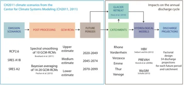
We combined 3 emission scenarios, 3 regional climate model estimates (based on 10 to 20 climate model runs), 2 post-processing methods and 3 hydrological models in a factorial way, leading to a total of 54 model chains applied to 6 catchments and 3 future periods, 2020-2049, 2045-2079 and 2070-2099 (Figure 1). In total, 972 hydrological projections of 30 years each were produced and analyzed. The factorial design of this modeling experiment reduces the risk of sampling artifacts, i.e., of reporting a result which only stems from a particular combination of models and is not representative of the other possible combinations. Further, it allows us to disentangle the contribution of the different elements of the model chain to the ensemble variance, and to quantify the eventual interactions between these factors.
2.2. Catchments
Discharge was simulated in six mesoscale catchments in Switzerland, which are representative of the main discharge types in mid-latitude alpine regions. These basins were shown to react differently to climate change by Köplin et al. (2012), who
7
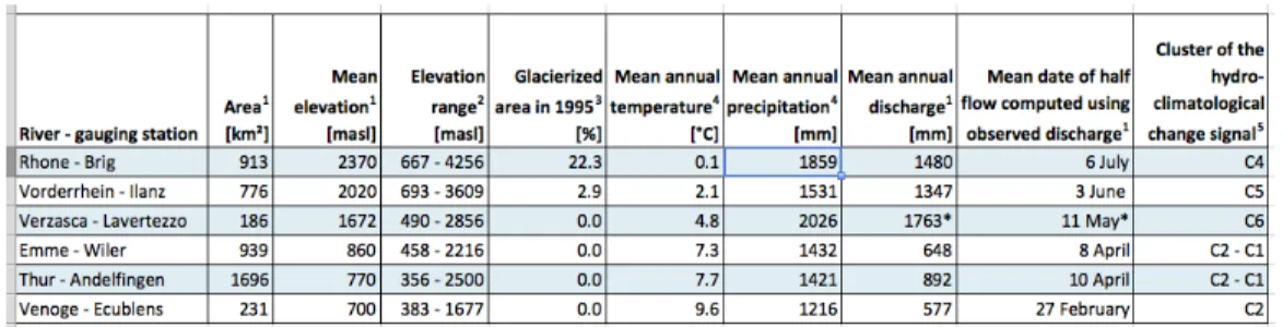
clustered 186 Swiss mesoscale catchments into 7 response types (Figure 2). Their mean elevation covers the range 700-2370 m a.s.l., their size varies between 231 and 1696 km2 and two of them are partially glacierized. They can be characterized as humid, as their evaporation is mainly energy-limited. The Venoge River flows on the plateau at the foothills of the Jura, a comparatively low-elevation mountain chain. Emme and Thur basins have their headwaters in the pre-Alps, whereas Rhone and Vorderrhein are alpine catchments, dominated by snow and ice-melt. The Verzasca basin is located on the southern side of the Alps. Further information on the catchment characteristics are provided in Table 1.
Dams are present in most of the large Swiss alpine catchments. According to the Swiss Committee on Dams (www.swissdams.ch), three dams are upstream of the Brig gauging station for the Rhone catchment and seven are upstream of Ilanz for the Vorderrhein catchment. The reservoirs are in average larger in Vorderrhein
catchment. Their total volume is about 31 x 106 m3 for the Rhone and 260 x 106 m3 for Vorderrhein, which corresponds to ~2.3% and ~24.9%, respectively, of the mean annual discharge at the gauging station for these two basins. The other four study basins, located at lower elevation, are essentially unregulated.
2.3. Climate projections
We used climate projections of the CH2011 data set (CH2011, 2011) from the Center for Climate Systems Modeling (C2SM). This recently released data set consists of two types of projections for Switzerland, both based on the climate model runs of the
8
ENSEMBLES project (van der Linden and Mitchell, 2009) and both relying on the delta change approach. According to this technique, projections are produced by combining observations to additive (multiplicative) factors for temperature (precipitation). These factors were assessed in a deterministic way by spectral
smoothing of 10 general circulation and regional climate model (GCM-RCMs) chains, and in a probabilistic way by a Bayesian multi-model approach combining 20 runs until 2050, and then 14 runs until 2099, respectively. CH2011 projections are not transient but available as mean temperature and precipitation changes over 2020-2049, 2045-2074 and 2070-2099, 1980-2009 being the reference period. This defines the periods over which hydrological simulations were run. The delta change factors were estimated from GCM-RCM simulations run with a daily time step. These factors were provided for each day of the year (365 values) and, once combined with station observations, yielded projections at the station scale. The interpolation within the catchments was performed by the hydrological models using the methods listed in Table 2. As the delta change method does not capture changes in variance, we restricted our analysis to the changes in the annual discharge cycle and did not consider extremes.
The production of the projections by the CH2011 team and their use to force
hydrological models in this study can be summarized as follows. For the deterministic data set, the delta change factors were determined for each of the 10 GCM-RCM chains by spectral smoothing. This technique enables the isolation of the precipitation and temperature annual cycles by removing fluctuations arising from natural
variability, that may results in artifacts in the estimated climate change signal (see Bosshard et al., 2011 for more details). Hydrological simulations were run for each of
9
the 10 GCM-RCM chains and then the lower (minimum of the 10), medium (median) and upper (maximum) estimates of discharge changes were derived. For the
probabilistic data set, the 14 to 20 GCM-RCM chains were combined into probability distributions using a Bayesian multi-model combination algorithm. As this algorithm requires data to be normally distributed, precipitation data were transformed to their square-root before their processing, and re-transformed after it. Similarly, the internal decadal variability was subtracted before the multi-model combination and was then re-added. The delta change factors corresponding to the 2.5, 50 and 97.5% quantiles were then extracted from the posterior distributions, after data re-transformation and the re-addition of the internal variability (see Fischer et al. (2012) and Zubler et al. (2014) for more details on the method and on its application to the alpine range, respectively). These projections, corresponding to the lower, medium and upper climate estimates, were used to force the hydrological models. Hence, in the deterministic case, each discharge simulation was driven by a single GCM-RCM chain, whereas in the probabilistic case, it was driven by, for e.g., the median of the GCM-RCM chains. The name of the climate models used and of the institutions responsible for the simulations are provided in Bosshard et al. (2011, Table 1) and Fischer et al. (2012, Figure 1).
The CH2011 projections were produced for three possible evolutions of greenhouse gas emissions and concentration: SRES A1B, SRES A2 and RCP2.6. The first two storylines were defined in the Special Report on Emissions Scenarios (SRES, Nakicenovic and Swart, 2000) and used in the framework of CMIP3. The third storyline is the Representative Concentration Pathway RCP2.6 (Meinshausen et al., 2011) used for the more recent CMIP5 (Taylor et al., 2012). A1B is a mid-range
10
emission scenario that was chosen for the ENSEMBLES simulations. To gain insights into lower and higher emissions pathways without the computational cost of rerunning the climate models under these scenarios, the CH2011 team used pattern scaling to generate projections under the climate stabilization scenario RCP2.6 and under the more extreme A2 scenario (CH2011, 2011; Fischer et al., 2012). This technique is a statistical emulator relying on the principal assumption is that any regional change is related to the global mean temperature signal in a linear way. Pattern scaling was applied to generate both precipitation and temperature projections at the regional scale, using scaling factors derived from temperature changes at the global scale (see Eq. 12 in Fischer et al., 2012). The accuracy of the pattern-scaled projections
primarily depends on the validity of the underlying assumption of linear relationship. Tebaldi and Arblaster (2014) concluded that it is broadly valid for CMIP3 and CMIP5 models and report geographical patterns of change consistent across different
emission scenarios. They also review limitations of the method and emphasize in particular that pattern-scaled projections are more reliable for temperature than for precipitation, at large than at small spatial scales and are likely less reliable in presence of feedbacks or when the focus is on extreme events. In this study, in absence of systematic GCM-RCM runs under A2 and RCP2.6, we consider the use of pattern-scaled projections as an adequate way to perform a first assessment of
sensitivities in hydrological simulations to greenhouse gas emission scenarios.
To summarize, the projections under A1B were obtained from GCM-RCM
simulations run under this scenario. In contrast, the projections under A2 and RCP2.6 do not rely on climate model runs under these scenarios, but were obtained using pattern-scaling. Further, whereas A1B and A2 are non-intervention scenarios,
11
considerable efforts are deployed under RCP2.6 to mitigate emissions. It follows that under this scenario, a global temperature increase by the end of the 21st century higher than 2°C relative to 1850–1900 is considered unlikely (i.e., 0 - 33% probability, IPCC, 2013). Note that in the CH2011 data set, RCP2.6 is referred to as RCP3PD, these two names corresponding to the same scenario (Meinshausen et al., 2011). We opted for RCP2.6, as it is named in the IPCC Fifth Assessment Report (IPCC, 2013).
The CH2011 setup does not allow for the separation of the GCM-RCM uncertainty into climate model uncertainty and natural climate variability. Climate model uncertainty is potentially reducible via a better understanding of global warming processes and models improvement, whereas natural climate variability is a stochastic and intrinsic part of the climate system, and is irreducible. Characterizing the future natural climate variability could for instance be achieved using projections from the same climate model started from different initial conditions (Deser et al., 2012) or by employing a weather generator constrained by GCM-RCM projections (Fatichi et al., 2014).
2.4. Hydrological modeling
Three hydrological models were used to evaluate the sensitivity of discharge projections to model structure, resolution and calibration: HBV (Seibert and Vis, 2012), PREVAH (Viviroli et al., 2009b) and WaSiM (Schulla, 2013). HBV and PREVAH are semi-distributed (HBV was applied using 100-m elevation zones and PREVAH using hydrological response units, HRU), whereas WaSiM is run on a 250x250m2 grid. HBV and PREVAH are based on a similar reservoir structure, while
12
WaSiM uses a more process-oriented approach. HBV and WaSiM were calibrated, whereas PREVAH parameter values were obtained by regionalization (Viviroli et al., 2009a). PREVAH simulations hence represent natural discharge conditions even in catchments with major reservoirs. The hydrological models are contrasted in more details in Table 2 and their coupling to the glacier model is discussed in section 2.5.
The reservoirs and the dam operations were not explicitly implemented in the hydrological models. Although their implementation might have enabled a better reproduction of the observed discharge under current climate, considerable uncertainties exist about the evolution of energy consumption and about the
importance of hydro-power production in comparison to other energy sources by the end of the century. One way to account for these uncertainties would be to formulate scenarios depicting different socio-economic developments at the Swiss and the international level, possibly in a similar fashion as the SRES emission scenarios (Nakicenovic and Swart, 2000). In this study, however, we restrain our attention to the uncertainties stemming from the future emissions and the models used to produce hydrological projections, and assume that the simulated discharge corresponds to natural discharge. This assumption is realistic in the Rhone catchment, where the total reservoir volume corresponds to only ~2.3% of the annual discharge, but is less robust in the Vorderhein catchment, which is more heavily managed (~24.9%). In the four other catchments, the discharge is not significantly affected.
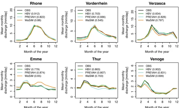
Initial results indicated that the performance of the hydrological models under present climate was overall good, and that they successfully capture the main features of the annual discharge cycles (Figure 3). Note that the models performance in the
13
Vorderrhein catchment is slightly impeded by discharge perturbations induced by hydro-power production. Differences between simulated and observed annual cycle over the reference period (1980-2009) are assumed to be constant in the future. The overall approach relies on the assumption of time stationarity of the biases in the climate and hydrological simulations, although evidence for nonstationaries exist (Maraun, 2012; Merz et al., 2011). We hence defined changes in discharge as the differences between the projected discharge and the discharge simulated using 1980-2009 meteorological observations. We considered the annual cycle as captured by monthly averages and computed seasonal averages for summer (June, July and August, referred to as JJA in continuation) and winter (December, January and February, DJF). Further, we investigated the earlier occurrence of peak river runoff in spring to summer, one of the most prominent discharge changes in a warmer climate in snow-dominated regions. This shift in seasonality is generally attributed to two main factors: the higher proportion of precipitation falling as rain instead of snow, and earlier snow melt and consecutive glacier melt (e.g., Barnett et al., 2005). To consider the combined effect of these two processes using one metric relying on discharge data, we considered the half-flow date (HFD) introduced by Court (1962), i.e., the date on which the cumulative discharge since the beginning of the hydrological year (starting on October 1) exceeds half of the total annual discharge. This date is often preferred to that of the maximum daily discharge, which can result from a punctual precipitation event. The HFD has been broadly used to investigate the effects of climate change on streamflow timing (e.g., Cortés et al., 2011; Stewart et al., 2005). Although Whitfield (2013) recently pointed out that HFD is not a reliable indicator of the timing of snowmelt, we use it here from a more general perspective
precipitation-14
dominated regimes (pluvial). In other words, we use HFD as a regime metric, with a later HFD corresponding to higher elevation and more snow-dominated regimes. This relation appears clearly from HFD computed using observed discharge in the six catchments (Table 1).
2.5. Modeling of glacier retreat and contribution to discharge
Ice melt significantly modifies the hydrological regime of glacierized catchments as it acts as a source of runoff after the disappearance of the snow cover (Barnett et al., 2005). The representation of glaciers in hydrological models is important to
realistically simulate discharge during the summer months, and changes therein with respect to atmospheric warming (e.g., Horton et al., 2006). The hydrological models applied in this study include modules for glacier melt but do not describe the more complex processes of dynamic changes in glacier thickness and size over time. Therefore, glacier melt was simulated in two steps. Glacier retreat was first modeled under the different climate projections and the resulting extent was provided as input to the three hydrological models. The contribution of glacier melt to discharge was then simulated in a second step by the hydrological models, i.e., not by the glacier model itself. Below, we provide more details and references about the modeling of glacier retreat and of the contribution of glacier melt to discharge.
The changes in future glacier coverage in the catchments were assessed by combining different glaciological models at high spatial resolution. The present glacier ice thickness distribution exerting an important control on the rate of glacier retreat and volume loss was evaluated. We used a model (Huss and Farinotti, 2012) to invert
15
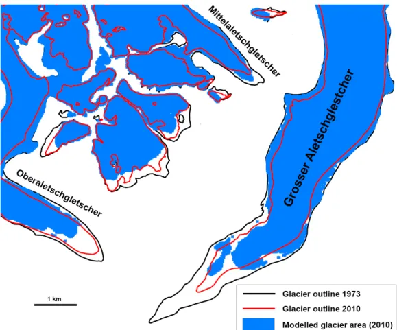
local ice thickness from glacier surface topography using the principles of ice flow dynamics. Glacier extent for the year 2010 was obtained from an inventory of all glacierized surfaces (Fischer et al., in press). Surface mass balances and 3D glacier geometry changes were calculated using a detailed glacier model (Huss et al., 2010b). This model was run at daily resolution on a 25m grid and takes into account snow accumulation distribution, the influence of radiation on ice melting according to Hock (1999) and calculated glacier retreat based on a mass-conservation approach. The glaciological model was calibrated with a variety of field data covering the entire 20th century (Huss et al., 2010a). Annual mass balances from the 50 glaciers were then extrapolated to every single glacier in the catchment by applying a multiple regression approach. Thus, glacier-specific transient annual series of the glacier mass budget were obtained and used to drive the model for every glacier (152 in the Rhone catchment, 105 in the Vorderrhein catchment). The model was validated over the period 1973-2010 for which the change in glacier extent is known. The overall change in ice-covered area is captured within 5%, and the retreat rates of the glacier termini are reproduced in general although some differences for individual sites are evident (Figure 4). Finally, the glacier model was forced until 2100 with the same climate scenarios as the three hydrological models. We also applied the same approach to downscale the climate data to individual glaciers. From the transient model runs we then extracted glacier ice coverage for 2035, 2060 and 2085 and assumed it to be constant over each of the 30-year period.
These glacier simulations were used as input for the three hydrological models. Again, the prescribed glacier extent is the same in each case, but the melt and the resulting contribution to discharge were computed separately by each model. HBV
16
relies on a degree-day approach considering temperature as the only driver of snow and ice melt. In the version used here, two multiplicative factors were added to the basic formulation of the degree-day approach in order to reflect the influence of exposure on snow and ice melt, and to account for the lower albedo on ice than on snow (Konz and Seibert, 2010). Melt water is transferred to the ground water reservoirs, the outflow of which being then routed to the catchment outlet using a triangular weighting function. PREVAH and WaSiM are principally based on the temperature-index method developed by Hock (1999), which is an extension of the degree-day method. It involves melt factors for snow and ice, and importantly, it includes radiation coefficients for snow and ice, and accounts for direct solar radiation. Melt water is routed to the underlying catchment using three linear reservoirs with different storage coefficients, for ice, firn and snow, respectively.
2.6. ANOVA
We chose the projection variance as an estimate of their uncertainty, and used an analysis of variance (ANOVA) technique to quantify the contribution of the different sources of uncertainty to the final uncertainty. The uncertainty partitioning relied on the following model
∆ (Eq. 1)
which expresses the change in discharge (∆ ) as the mean change ( ) modulated by the main effects of four factors, the emission scenario ( , i=RCP2.6, A1B, A2), the climate model estimate ( , j=lower, medium, upper), the post-processing (P ,
17
k=deterministic, probabilistic), the hydrological model ( , l=HBV, PREVAH,
WaSiM), as well as the sum of the significant interactions between these factors ( ) and the residual error . The interaction terms allow accounting for non-additive effects, i.e., for situations in which the combined effect of two factors is not the sum of their individual effects. We only considered first-order interactions, i.e.,
interactions between two factors, as accounting for and interpreting higher order interactions is hard to physically justify. The assessment of the significance of first-order interactions, and their inclusion or not in the ANOVA model, was based on F-tests. The sum of squares of each element (main effects, interactions and error term) was divided by the total sum of squares of ∆ to compute the fraction of variance explained by this element (von Storch and Zwiers, 2001; Bosshard et al., 2013). This analysis was performed for each catchment, future period and for both summer (JJA) and winter (DJF) projections.
2.7. Natural variability under present climate
To assess the significance of the projected temperature, precipitation and discharge changes, we compared them with an estimate of the natural variability obtained by bootstrapping of observations. This estimate can be seen as noise (N) and was used to normalize the change of discharge (S), transforming it into a unitless signal-to-noise ratio (S/N as e.g., in Hawkins and Sutton, 2012). We followed Bosshard et al. (2011) to estimate N and constructed 100 30-year time series by re-sampling years with replacement from the 1980-2009 records. This approach relies on the assumption that a baseline distribution can be estimated from these 30 years and that realizations equally likely under this climate can be created by resampling from this distribution.
18
Then, 500 pairs of synthetized time series were randomly selected and the differences between these pairs computed. The standard deviation among these 500 differences was then used as an estimate of N. In the following, N is considered as the typical difference between two time series in absence of climate change, i.e., as a result of climate internal variability. Therefore, the standard deviation among the 500
differences of the annual, seasonal and monthly means were computed, respectively. N was computed at the seasonal scale (winter and summer) for precipitation and temperature, and at the yearly, seasonal and monthly scale for discharge. As periods of 30 years were considered, N reflects the natural variability over decadal time scales. The years used to construct the 100 time series and the subsequent 500 combinations were identical for the six catchments to account for inter-site
correlations. The Verzasca is the only exception, as its discharge record begins shortly before the beginning of hydrological year 1990, the 30-year time series were
synthetized by bootstrapping measurements from the 1990-2009 period.
3. Results
3.1. Changes in the annual regimes and in glacier coverage
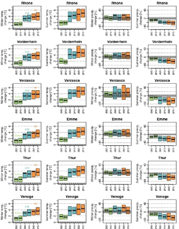
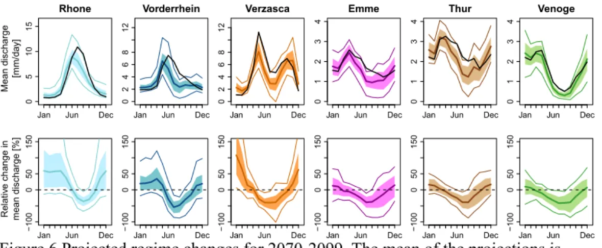
For each catchment, the agreement among the model chains of our setting is depicted Figure 6 for 2070-2099. The ensemble confirms climate change impacts on discharge already reported in previous studies on Swiss catchments (Bosshard et al., 2013; Bundesamt fu r Umwelt BAFU, 2012; Horton et al., 2006; Köplin et al., 2012) and in addition reveals strong model agreement for three of these impacts by the end of the century. Firstly, for all catchments, lower summer (JJA) flows are projected by
19
more than 90% of the model chains, irrespective of the emission scenario, climate model, post-processing or hydrological model. This is mainly related to a summer precipitation decrease (Köplin et al., 2012), as the changes in actual
evapotranspiration were found to play a secondary role (Adam et al., 2009; Köplin et al., 2013). Secondly, more than 85% of the simulations indicate an earlier timing of spring-summer peak discharge, as a consequence of temperature increase. Thirdly, larger winter (DJF) flows are projected by about two thirds of the runs in three lowest basins, and by more than 80% of them in the three highest basins. This mainly results from the higher fraction of liquid to solid precipitation during winter, leading to higher direct runoff. Note that the smaller snow storage causes lower melt peaks, especially at higher elevations. Winter precipitation might increase and contribute to higher winter discharge, but this remains uncertain, as the projected changes mostly fall within the estimated range of natural variability (Figure 5). Note that in contrast, the temperature changes simulated at the regional scale clearly emerge from noise in both winter and summer, as already reported by Bosshard et al. (2011) and Fischer et al. (2012). Although the expected changes in the Swiss plateau (Venoge) and pre-alpine catchments (Emme, Thur) are comparatively small in absolute terms, the relative changes are considerable (bottom row
Figure 6). In particular, the discharge during the low flow period, in summer, is likely to decrease by 25 to 50% for these three catchments.
The distributed modeling of glacier retreat forced by the probabilistic climate scenarios led to the projections summarized in Figure 7. By the end of the century, and for the medium climate scenario, the glacierized area in the Rhone catchment is projected to be reduced to ~45% of its 2010 extent under RCP2.6, and to ~27% under
20
A1B and A2. In the Vorderrhein catchment, the relative loss is higher, the glaciers are expected to retreat to ~17% and ~7% of their 2010 area, respectively, and only cover a few km2 by the end of the century. The uncertainty stemming from the GCM-RCMs is represented by the shaded areas and is large under each emission scenario. For instance, in the Rhone catchment, the lower and upper climate estimates (95% confidence interval) under RCP2.6 lead to a remaining glacierized area stretching from 26% to 68% of its 2010 value. Note that the uncertainties related to the formulation and the parameter values of the glacier model were not assessed in this paper.
3.2. Uncertainty decomposition
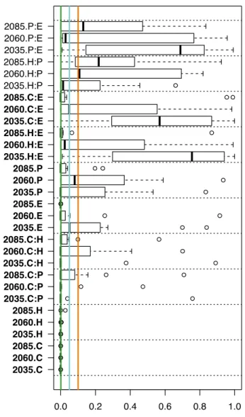
To quantify the respective contribution of the four uncertainty sources to the uncertainty captured by our experiment, analyses of variance (ANOVA) were performed, which allowed for uncertainty partitioning for each of the three future periods and for each catchment. We first assessed the significance of the main effects and interactions of the ANOVA model. For each main effect or first-order interaction, the null hypothesis is that its coefficients are all null, e.g., that the emission scenario has no influence on the projected discharge change (Ei=0 for all i in Eq. 1). The
hypothesis was evaluated using F-tests, and their p-values were summarized in Figure 8. We kept all the main effects and most of the interactions, including the interactions
H:E and C:E because they are in most cases significant for the middle and end of
century projections. The interactions P:E and H:P were excluded because they are not significant in most cases.
21
The uncertainty stemming from the GCM-RCMs, i.e., the combination of model uncertainty and natural climate variability, dominates in general (Figure 9). Our setup shows that the relative importance of this source varies with catchment characteristics. While the projection uncertainty is principally driven by the GCM-RCMs in the non-glacierized catchments, the hydrological models explain as much variance and sometimes more than the GCM-RCMs in the partially galcierized catchments, Rhone and Vorderrhein. The different hydrological models lead to different projections in these catchments, in particular for the change in Rhone summer discharge, with HBV and WaSiM simulating a much larger (~2.8 mm/day) mean decrease than PREVAH (~0.5 mm/day). For the other catchments, the hydrological models explain little of the variance, which means that, in these catchments, the differences in model structure, resolution and calibration barely influence the discharge projections.
The fraction of variance explained by the emission scenarios increases with time, for both seasons and in all catchments, and so does the significance of the emission scenario factor in the ANOVA model (Figure 8). This source of uncertainty explains a higher fraction of variance in summer than in winter, but is usually not the dominant one by the end of the century for the catchments investigated. The difference in complexity between the two post-processing methods, and the different sets of climate models they rely on, appears to have little influence. Finally, the variance explained by the interactions needs to be considered, in particular in summer.
3.3. Emergence of the climate change signal from natural discharge variability
22
The annual discharge cycles of the time series constructed by boot-strapping are shown in Figure 10. Overall, the variability is higher in lower elevation basins, as illustrated by the higher dispersion of the 100 constructed time series around the cycle directly derived from observations When computed for each month, the variability corresponds in average to 7 to 19% of the discharge on the same month, with higher values typically reached in higher-elevation catchments. A clear exception to this relation is the Verzasca, which exhibits a rather high variability given its elevation. This relationship between elevation and variability translates to HFD, which present higher variability at lower elevation. It ranges from 1.8 days in the Rhone catchment to 8.1 days for the Venoge, the Verzasca being again an outlier with a value of 11.8 days. As noted earlier, higher elevation catchments are associated to a later HFD.
Estimating the natural discharge variability in the six catchments allows for the investigation of the emergence of the climate change signal. It already emerges from noise in certain months of the first future period (2020-2049) in the alpine catchments (Rhone and Vorderrhein) and irrespectively of the emission (Figure 11). The impacts become more severe with time and our results indicate that at the end of the century, the climate change signal clearly emerges from natural variability for all catchments in summer, even if emissions are limited to the lowest level (RCP2.6). The S/N ratios are higher in the higher-elevation catchments.
3.4. Sensitivity of the impacts on discharge to the emission scenarios
We explored the influence of the emission scenarios on the hydrological regime by computing the average discharge change for each emission scenario, catchment and
23
future period. As expected from the analyses of variance, the differences between the emission scenarios increase with time (Figure 11). These differences are negligible for the first future period (2020-2049), the impacts occurring independently of the
emission policy or lack thereof. Differences between the intervention (RCP2.6) and the non-intervention (A1B and A2) scenarios become clear for the 2045-2074 projections, when impacts increase (not shown). By the end of the century (2070-2099), a further increase of the climate change impacts is projected, but there is only little difference between A1B and A2, which is consistent with the similarity of their temperature and precipitation projections for the study basins (Figure 5). An
important result is that, according to our simulations, following the intervention scenario would reduce the largest impacts on the regime (in summer and winter) by the end of the century by about a factor of two.
4. Discussion
4.1. A large but inevitably incomplete set of model chains
This study relies on a large set of model chains, with 3 emission scenarios, 10-20 GCM-RCMs, 2 post-processing methods and 3 hydrological models combined factorially and applied to 6 catchments. We nevertheless acknowledge that model sampling is neither complete nor random, which is a general barrier to a full
uncertainty sampling (Knutti et al., 2010). The models are also equally-weighted, in a finite number and somewhat interdependent (see the discussion on climate models in Masson and Knutti, 2011, and the hydrological model characteristics in Table 2). It thus cannot be excluded that some agreement between the simulations stems from
24
model similarities, such as a common bias among the climate or hydrological models, and hence should not be interpreted as low uncertainty. It is debatable whether adding more chains would change our characterization of the projection uncertainty, improve our understanding of future catchment discharge and provide a stronger support for decision-making under uncertainty. Here we argue that even though sets of model chains are inevitably incomplete, the use of a wide and balanced set of combinations provides new insights into the influence of the catchment on the uncertainty of the discharge projections, relates to fundamental questions on the relation between model complexity and performance and helps to find robust features that can better support decision-making. These points are discussed below.
4.2. How much do catchments determine uncertainty partitioning?
The decomposition of variance revealed that the discharge uncertainty is in general dominated by the uncertainty from the GCM-RCM projections, which is in agreement with previous studies (Wilby and Harris, 2006; Prudhomme and Davies, 2009; Dobler et al., 2012; Bosshard et al., 2013; Huss et al., 2013). Our setup further allows for the investigation of changes in the uncertainty partitioning from catchment to catchment (Figure 9).
The hydrological models explain a considerable portion of the variance in the Rhone and Vorderrhein catchments, but their influence is much smaller in the other
catchments. In our view, this results from key characteristics of these two catchments that differentiate them from the others: their nival to glacial regime, their more complex topography and the presence of dams. In alpine catchments, a realistic
25
regime representation is conditioned by the realistic simulation of accumulation and melt processes of snow, and of ice in glacierized catchments. These processes are subject to structural uncertainties (they are formulated in different ways in the
hydrological models, see Table 2) and parametric uncertainties (parameter estimation is performed using different methods, see Table 2, and is challenging as a result of equifinality (Beven, 2006) and of the highly multi-dimensional parameter space (Kirchner, 2006)). Overall, the value of parameters regulating snow and ice is poorly constrained when model calibration is performed on the basis of simulated discharge alone. This can lead to compensation errors, which then contribute to differences in the discharge simulated by the different models. Clearly, structural and parametric uncertainties also influence discharge simulations in lower-elevation catchments, but the potential for compensation errors resulting in misallocations of water between glacier, snow and runoff is arguably larger at higher elevation, where storage of water as ice and snow is higher. A better agreement between the models might be achieved by multi-criteria calibration, involving for instance the incorporation of glacier mass balance and snow cover extent retrieved from satellite imagery, as implemented by Parajka and Blöschl (2008) and Finger et al. (2012). This would enable snow and ice mass balances to be more realistically simulated, an aspect not evaluated by
calibration methods based on discharge simulations alone. Another characteristic influencing uncertainty partitioning is topography. Although the hydrological models are forced by the same climate projections, the more complex topography in higher altitude catchments leads to higher errors in the interpolation of these projections, an operation performed by the hydrological models. Finally, the discharge perturbations induced by hydropower production during the calibration period decrease the
26
implemented in this study. These numerous factors contribute to explain why the uncertainty stemming from the hydrological models is higher in the alpine catchments.
Catchments also influence the importance of the emission scenario. In winter it is lower in the Thur, Emme and Venoge basins (mainly precipitation-driven) than in the higher elevation basins, Rhone, Vorderrhein and Verzasca (more temperature-driven). This is consistent with the climate projections for winter, which are similar under the three emission scenarios for precipitation, but differ for temperature (Figure 5). The difference between low and high-elevation catchments is reduced in summer, when both precipitation and temperature changes depend strongly on the emission scenarios.
The influence of the post-processing method and the set of GCM-RCM chains they rely upon does not seem to depend on catchment characteristics and is weak in all cases. This reflects the great similarity of the projections from the deterministic and probabilistic data sets for the study basins (Figure 5). The differences in the projected discharges could however be stronger for extremes (Wilby and Harris, 2006; Dobler et al., 2012) and if other post-processing methods, such as quantile-mapping (Dosio and Paruolo, 2011), were also considered. Also, if a smaller number of GCM-RCMs had been used, the selection of the climate models might have had a larger effect on the discharge projections. Wilby and Harris (2006), for instance, used four GCMs and showed that, while three of them lead to rather similar changes in future low flows, the last one resulted in quite different projections (their Figure 5b). In such a case, including this last GCM in the analysis or not, can lead to quite different conclusions
27
about the origin of the uncertainty in the discharge projections.
It should be stressed that the validity of the uncertainty partitioning relies in particular on the experimental design. A critical point here is the assessment of the interactions terms. The two most significant interactions are between the climate model, the post-processing method (C:P) and the hydrological model (C:H, Figure 8). The combined effect of these elements on discharge is thus non-additive. For instance, when the medium climate estimate and the hydrological model HBV are combined, their effect on the discharge projection is not only the sum of their respective effects, but rather this sum corrected by an additive interaction term (Eq. 1). An important consequence is that, if the uncertainty stemming from the chain elements (e.g., from the
hydrological models) had been computed by varying the models for this element (e.g., using sequentially HBV, PREVAH and WaSiM) while keeping the rest of the chain constant (e.g., using only SRES A1B, medium climate estimate and the probabilistic post-processing), a biased estimate of the uncertainty could result, as significant interactions (e.g., between the climate and the hydrological models) would not have been sampled. The non-negligible role played by the interactions hence stresses that the choice of the setup is key for a reliable assessment of uncertainties in the modeling chain. Note that although we rely here on a factorial design, a less computing
intensive approach based on a fractional factorial design requiring only a subset of the runs could be envisaged for future studies (Wu and Hamada, 2009).
4.3. Which model structure and calibration for hydrological impact studies?
28
hydrological models is almost negligible (Figure 9). The three models (HBV, PREVAH, WaSiM) rely on different spatial discretizations (100m elevation bands, hydrological response units or 250x250m2 grid), different parameter estimation procedures (genetic algorithm, regionalization, PEST), different numbers of land cover classes (1, 22 and 25) and different reservoir structures. Yet their projected regimes seem barely sensitive to these differences. We see three complementary explanations of this outcome.
First, external forcing, i.e., atmospheric projections, can act as the main driver of the simulated discharge, overwhelming any differences between the hydrological models. Climate projections are significantly different from the climate during the reference period (Figure 5), our results suggest that these differences can overrule the structural differences among the hydrological models.
Second, our study focused on changes in the mean seasonal discharge over 30-year periods. A model might perform better at capturing individual events, for instance the few large flooding events during this period, but this is averaged out when
considering changes of mean discharge. Larger differences between the models might thus have emerged if other components of the hydrograph had been systematically investigated, for example low flows (Velázquez et al., 2013).
Third, the similarity of the projections delivered by different models raises the question of how much complexity is needed in hydrological models executed under climate change. This is related to the much-debated relation between model
29
model elements are necessary to deliver reliable discharge simulations in a changing climate? The answer arguably depends on the catchment characteristics and on the hydrological parameter investigated, as there is most likely no model structure that provides reliable projections in all cases (Savenije, 2009). Several contributions exist to support the choice of model structure. They rely, for instance, on model inter-comparisons (Smith et al., 2004, 2012), on the Framework for Understanding Structural Errors (FUSE; Clark et al., 2008; Staudinger et al., 2011), on differential split sample tests (Seiller et al., 2012), on a model evaluation without calibration method (Vogel and Sankarasubramanian, 2003) or adopt a more process-oriented approach (Herman et al., 2013). Concerning hydrological model calibration, Merz et al. (2011) and Coron et al. (2012) highlight the issue of parameter stationarity over time and discuss the consequence thereof for simulation of hydrological impacts. Others consider the whole impact modeling chain (Figure 1) to estimate the sensitivity of hydrological projections to the model structure (Velázquez et al., 2013) or to the method chosen to estimate parameters value (Poulin et al., 2011). These later studies consider the hydrological model in the context of the cascade of uncertainty and compare its contribution to that of the other elements of the model chain, hence providing particularly valuable insights for the further development of hydrological modeling in changing conditions.
4.4. Why is natural discharge variability higher in lower elevation catchments?
The overall negative correlation between catchment elevation and natural discharge variability under present conditions (Figure 10) can be explained by a damping by
30
glaciers and the snow pack. According to Lang (1986) this damping can occur
through three main mechanisms. During dry years characterized by lower than normal precipitation and higher net radiation and sensible heat, glacier balance is usually negative and the contribution of melt water to discharge is significant. Conversely, during years with much precipitation, the input to glaciers is usually higher and melt is lower, which corresponds to a positive glacier mass balance and a smaller
contribution to discharge. Glacier melt hence tends to compensate for year-to-year rainfall anomalies. Another compensating effect stems from the tendency of climatic situations leading to higher glacial melt to also cause higher evapotranspiration in basins spanning over a wide range of elevations. Finally, the snow pack can also damp discharge variations, by temporarily containing intense precipitation events and then releasing the water progressively.
The comparatively high discharge variability of the Verzasca given its elevation probably comes from the location of the basin, on the southern flank of the Alps. Its climate is directly influenced by Mediterranean airflows and the natural precipitation variability of its region is larger than on the northern side of the Alps (Fischer et al., 2012). Further, when comparing the projected changes to the natural variability (Figure 11), it appears that the changes in regime are more pronounced in the higher elevation catchments, a result also reported by Fatichi et al. (2014).
4.5. Can the identification of robust changes help adaptation?
We investigated the robustness of the projections by considering robustness as the combination of a strong agreement between simulations and a projected change
31
exceeding natural variability (Knutti and Sedláček, 2012). These two aspects were investigated separately in sections 3.1 and 3.3, respectively. To conclude this study, they were combined in Figure 12 for the three regime impacts discussed above: lower summer discharge, higher winter discharge and change toward more rain-dominated regime. In addition, we also considered changes in the mean annual volume, which correspond to changes in the water balance integrated over 30 years. In the four cases, the robustness of the projections is higher for the higher elevation catchments, i.e. their mean future change normalized by the natural variability is higher, and more model chains agree on the sign of the change. We explain this outcome by the robustness of the future climate simulations, which is higher for temperature than for precipitation (Figure 5), resulting into more robust discharge changes in temperature-driven, higher elevation catchments. Similarly, as the robustness of the climate change signal tends to increase with time in the catchments investigated (Figure 5), so does the robustness of the hydrological projections.
Note however that different robustness patterns emerge. In the lower altitude catchments, there is a strong model agreement and high signal-to-noise ratios about lower summer discharge, but the projections confidence is weaker when it comes to higher winter discharge, as could be expected from the results shown in
Figure 6. Further, note that model agreement on the shift toward more rain-dominated hydrological regimes is particularly high and is already complete (100%) in 2035 for the three highest catchments. Overall, high signal-to-noise ratios are reached for these three first changes. It implies that the projected changes are unlikely to stem from natural variability alone, but are rather a consequence of anthropogenic emissions.
32
According to our ensemble of simulations, the total discharge volume is expected to decrease in the future. This change is less robust than the other three (Figure 12 a to c versus d), yet by 2085 it emerges from natural discharge variability and is projected by 60 to 85% of the model chains. Possible causes include the expected decrease in summer precipitation and smaller glacier contribution to discharge, and perhaps the precipitation shift from snow toward rain (Berghuijs et al., 2014). At this stage, the respective contribution of these processes is unclear.
Because of the diversity of the model combinations considered, our projections are subject to substantial uncertainties, as shown by the large spread of the ensemble ( Figure 6). Nevertheless, Figure 12 shows that by the end of the century, robust changes in regime emerge from the noise, that they are supported by a large agreement among the model runs and that they are valid across the whole range of catchments. We argue that identifying such features can contribute to support decision-making on adaptation strategies.
4.6. Can our results and method be generalized?
Our study focused on six catchments, but data sets with hundreds of catchments are becoming more easily available (Gupta et al., 2014). They can be combined with climate projections to perform a similar systematic analysis in a larger number of catchments spanning a wider range of climatic conditions. However, since uncertainty sampling and decomposition requires a large number of simulations, available
computing infrastructures will often limit the analysis to a selection of catchments. So which catchments to select? A solution is to reduce the dimensionality of the problem.
33
Köplin et al. (2012) for instance run a single hydrological model under a single emission scenario using 10 GCM-RCMs post-processed by a single method in 186 mesoscale Swiss catchments. A cluster analysis then enabled them to reduce these 186 catchments to 7 response types, from which the catchments used in this study were chosen (Figure 2). We then produced hydrological projections for this selection of catchments using several emission scenarios, hydrological models and GCM-RCM post-processing methods. The similarity of our results for the Emme, Thur and Venoge catchments is in agreement with their clustering, as they associated these basins to the same type of response to climate change. This suggests that our results may be extrapolated to other Swiss watersheds on the basis of their cluster analysis and advocates for the application of a similar approach to other regions.
5. Conclusions
This study considers and systematically analyses a large number of uncertainty sources when simulating future hydrological regimes in Swiss catchment. Analyses of variance based on a factorial experimental design were used to decompose the
uncertainty of the projections. This showed that although GCM-RCMs are usually the main source of uncertainty, the uncertainty stemming from the hydrological models in the catchments dominated by snow and ice melt is substantial. In contrast, the choice of the hydrological model is barely significant in the lower altitude basins. The importance of the emission scenario increased with time into the future, yet without becoming the major source of uncertainty. The post-processing of the climate projections plays the least relevant role in our study.
34
We assessed the robustness of expected changes in regime already reported in the literature: the decrease of summer discharge, the increase of winter discharge and shift toward lower-elevation, more rain-driven regimes. These changes are characterized by a large agreement among the simulations and by projected changes significantly larger than the natural variability, which was estimated by the bootstrapping of discharge records. Given the wide range of models involved in our setup, we concluded that these changes are robust despite the uncertainty of the projections, especially in the higher elevation basins.
We compared the projections under the intervention scenario RCP2.6, implying considerable efforts to reduce emissions, and under two non-intervention scenarios, SRES A1B and A2. Over the coming decades, the impacts are projected
independently of the scenario and the climate change signal already emerges from natural discharge variability in the high-elevation basins. By the end of the century, the projected impacts are more pronounced, the climate change signal emerges in all basins in summer and there are clear differences between the intervention and the non-intervention scenarios. Our results indicate with confidence that impacts on discharge can be reduced considerably if a stringent emission policy is adopted.
This study relies on a coordinated modeling experiment, enabling the investigation of projection uncertainties in a systematic and quantitative way, and in several
catchments. This hydrological modeling framework provides new insights into future hydrological regimes, and because it allows for the identification of robust changes, we argue that it is an important step for the support of decision-making based on uncertain projections.
35 Acknowledgements
We thank the CH2014-Impacts project (CH2014 Impacts, 2014) for providing the framework in which this study was initiated. We are indebted to the Center for Climate Systems Modeling (C2SM) for producing and providing the CH2011 data. This data set relies on the climate simulations from the EU-funded FP6 Integrated Project ENSEMBLES whose support is gratefully acknowledged. We thank Reinhard Furrer for his help with the statistical analysis, Thomas Bosshard und Luzi Bernhard for inspiring discussions, Jan Schwanbeck for his help with the creation of PREVAH input files, as well as the Associate Editor and the three Reviewers for their
comments, which contributed to improve this paper. We acknowledge the Swiss Federal Offices for the Environment (FOEN), of Meteorology and Climatology (MeteoSwiss) and of Topography (swisstopo) for the hydrological, meteorological and topographic data. This study was partially funded by the Swiss National Science Foundation (grant 200021_131995). The discharge projections produced in this study are available upon request from the first author.
References
Adam, J. C., Hamlet, A. F. and Lettenmaier, D. P.: Implications of global climate change for snowmelt hydrology in the twenty-first century, Hydrol. Process., 23, 962– 972, doi:10.1002/hyp, 2009.
36
Addor, N., Jaun, S., Fundel, F. and Zappa, M.: An operational hydrological ensemble prediction system for the city of Zurich (Switzerland): skill, case studies and
scenarios, Hydrol. Earth Syst. Sc., 15(7), 2327–2347, doi:10.5194/hess-15-2327-2011, 2011.
Barnett, T. P., Adam, J. C. and Lettenmaier, D. P.: Potential impacts of a warming climate on water availability in snow-dominated regions., Nature, 438(7066), 303–9, doi:10.1038/nature04141, 2005.
Berghuijs, W. R., Woods, R. A. and Hrachowitz, M.: A precipitation shift from snow towards rain leads to a decrease in streamflow, Nat. Clim. Chang., 18–21,
doi:10.1038/NCLIMATE2246, 2014.
Beven, K.: A manifesto for the equifinality thesis, J. Hydrol., 320(1-2), 18–36, doi:10.1016/j.jhydrol.2005.07.007, 2006.
Bosshard, T., Carambia, M., Goergen, K., Kotlarski, S., Krahe, P., Zappa, M. and Schär, C.: Quantifying uncertainty sources in an ensemble of hydrological climate-impact projections, Water. Resour. Res., 49, 1523–1536,
doi:10.1029/2011WR011533, 2013.
Bosshard, T., Kotlarski, S., Ewen, T. and Schär, C.: Spectral representation of the annual cycle in the climate change signal, Hydrol. Earth Syst. Sc., 15(9), 2777–2788, doi:10.5194/hess-15-2777-2011, 2011.
Bundesamt fu r Umwelt BAFU (Eds.): Auswirkungen der Klimaänderung auf Wasserressourcen und Gewässer: Synthesebericht zum Projekt “Klimaveränderung
37
und Hydrologie in der Schweiz” (CCHydro), Bundesamt für Umwelt, Bern, Switzerland., 2012.
CH2011: Swiss Climate Change Scenarios CH2011, C2SM, MeteoSwiss, ETH, NCCR Climate, and OcCC, Zurich, Switzerland., 2011.
CH2014 Impacts: Toward quantitative scenarios of climate change impacts in Switzerland, FOEN, MeteoSwiss, C2SM, Agroscope, and ProClim, Bern, Switzerland., 2014.
Clark, M. P., Slater, A. G., Rupp, D. E., Woods, R. A., Vrugt, J. A., Gupta, H. V., Wagener, T. and Hay, L. E.: Framework for Understanding Structural Errors (FUSE): A modular framework to diagnose differences between hydrological models, Water Resour. Res., 44(12), doi:10.1029/2007WR006735, 2008.
Coron, L., Andréassian, V., Perrin, C., Lerat, J., Vaze, J., Bourqui, M. and Hendrickx, F.: Crash testing hydrological models in contrasted climate conditions: An experiment on 216 Australian catchments, Water. Resour. Res., 48(5), 1–17,
doi:10.1029/2011WR011721, 2012.
Cortés, G., Vargas, X. and McPhee, J.: Climatic sensitivity of streamflow timing in the extratropical western Andes Cordillera, J. Hydrol., 405(1-2), 93–109,
doi:10.1016/j.jhydrol.2011.05.013, 2011.
Court, A.: Measures of streamflow timing, J. Geophys. Res., 67(11), 4335–4339, doi:10.1029/JZ067i011p04335, 1962.
38
Deser, C., Knutti, R., Solomon, S. and Phillips, A. S.: Communication of the role of natural variability in future North American climate, Nat. Clim. Chang., 2(11), 775– 779, doi:10.1038/nclimate1562, 2012.
Dobler, C., Hagemann, S., Wilby, R. L. and Stötter, J.: Quantifying different sources of uncertainty in hydrological projections in an Alpine watershed, Hydrol. Earth Syst. Sc., 16(11), 4343–4360, doi:10.5194/hess-16-4343-2012, 2012.
Doherty, J.: PEST: Software for Model-Independent Parameter Estimation. [online] Available from: http://www.sspa.com/pest, 2005.
Dosio, A. and Paruolo, P.: Bias correction of the ENSEMBLES high-resolution climate change projections for use by impact models: Evaluation on the present climate, J. Geophys. Res., 116(D16), 1–22, doi:10.1029/2011JD015934, 2011.
Fatichi, S., Rimkus, S., Burlando, P. and Bordoy, R.: Does internal climate variability overwhelm climate change signals in streamflow? The upper Po and Rhone basin case studies., Sci. Total Environ., doi:10.1016/j.scitotenv.2013.12.014, 2014.
Finger, D., Heinrich, G., Gobiet, A. and Bauder, A.: Projections of future water resources and their uncertainty in a glacierized catchment in the Swiss Alps and the subsequent effects on hydropower production during the 21st century, Water. Resour. Res., 48(2), doi:10.1029/2011WR010733, 2012.
Fischer, A. M., Weigel, A. P., Buser, C. M., Knutti, R., Künsch, H. R., Liniger, M. A., Schär, C. and Appenzeller, C.: Climate change projections for Switzerland based on a Bayesian multi-model approach, Int. J. Clim., 32(15), 2348–2371,
39
Fischer, M., Huss, M., Barboux, C. and Hoelzle, M.: The new Swiss Glacier Inventory SGI2010: Relevance of using high-resolution source data in areas dominated by very small glaciers, Arctic, Antarct. Alp. Res., in press, n.d.
Frei, C.: Interpolation of temperature in a mountainous region using nonlinear profiles and non-Euclidean distances, Int. J. Climatol., Early view, doi:10.1002/joc.3786, 2013.
Frei, C. and Schär, C.: A precipitation climatology of the Alps from high-resolution rain-gauge observations, Int. J. Climatol., 18(8), 873–900, doi:10.1002/(SICI)1097-0088(19980630)18:8<873::AID-JOC255>3.0.CO;2-9, 1998.
Frei, C., Schöll, R., Fukutome, S., Schmidli, J. and Vidale, P. L.: Future change of precipitation extremes in Europe: Intercomparison of scenarios from regional climate models, J. Geophys. Res., 111(D6), D06105, doi:10.1029/2005JD005965, 2006.
Gebrehiwot, S. G., Seibert, J., Gärdenäs, A. I., Mellander, P.-E. and Bishop, K.: Hydrological change detection using modeling: Half a century of runoff from four rivers in the Blue Nile Basin, Water Resour. Res., 49(6), 3842–3851,
doi:10.1002/wrcr.20319, 2013.
Gupta, H. V., Perrin, C., Blöschl, G., Montanari, a., Kumar, R., Clark, M. and Andréassian, V.: Large-sample hydrology: a need to balance depth with breadth, Hydrol. Earth Syst. Sci., 18(2), 463–477, doi:10.5194/hess-18-463-2014, 2014.
Harlin, J. and Kung, C.-S.: Parameter uncertainty and simulation of design floods in Sweden, J. Hydrol., 137(1-4), 209–230, doi:10.1016/0022-1694(92)90057-3, 1992.
40
Hawkins, E. and Sutton, R.: The potential to narrow uncertainty in projections of regional precipitation change, Clim. Dyn., 37(1-2), 407–418, doi:10.1007/s00382-010-0810-6, 2010.
Hawkins, E. and Sutton, R.: Time of emergence of climate signals, Geophys. Res. Lett., 39, 1–6, doi:10.1029/2011GL050087, 2012.
Herman, J. D., Reed, P. M. and Wagener, T.: Time-varying sensitivity analysis clarifies the effects of watershed model formulation on model behavior, Water Resour. Res., 49(3), 1400–1414, doi:10.1002/wrcr.20124, 2013.
Hock, R.: A distributed temperature-index ice- and snowmelt model including potential direct solar radiation, J. Glaciol., 45(149), 101–111, 1999.
Horton, P., Schaefli, B., Mezghani, A., Hingray, B. and Musy, A.: Assessment of climate-change impacts on alpine discharge regimes with climate model uncertainty, Hydrol. Process., 20(10), 2091–2109, doi:10.1002/hyp.6197, 2006.
Huss, M. and Farinotti, D.: Distributed ice thickness and volume of all glaciers around the globe, J. Geophys. Res., 117(F4), F04010, doi:10.1029/2012JF002523, 2012.
Huss, M., Hock, R., Bauder, A. and Funk, M.: 100-year mass changes in the Swiss Alps linked to the Atlantic Multidecadal Oscillation, Geophys. Res. Lett., 37(10), doi:10.1029/2010GL042616, 2010a.
Huss, M., Jouvet, G., Farinotti, D. and Bauder, A.: Future high-mountain hydrology: a new parameterization of glacier retreat, Hydrol. Earth Syst. Sc., 14(5), 815–829, doi:10.5194/hess-14-815-2010, 2010b.
41
Huss, M., Zemp, M., Joerg, P. C. and Salzmann, N.: High uncertainty in 21st century runoff projections from glacierized basins, J. Hydrol., 510, 35–48,
doi:10.1016/j.jhydrol.2013.12.017, 2013.
IPCC: Climate Change 2013: The physical science basis. Contribution of Working Group I to the Fifth Assessment Report of the Intergovernmental Panel on Climate Change., Cambridge University Press, Cambridge, UK, and New York, NY, USA., 2013.
Kirchner, J. W.: Getting the right answers for the right reasons: Linking
measurements, analyses, and models to advance the science of hydrology, Water Resour. Res., 42(3), doi:10.1029/2005WR004362, 2006.
Knutti, R., Furrer, R., Tebaldi, C., Cermak, J. and Meehl, G. A.: Challenges in Combining Projections from Multiple Climate Models, J. Clim., 23(10), 2739–2758, doi:10.1175/2009JCLI3361.1, 2010.
Knutti, R. and Sedláček, J.: Robustness and uncertainties in the new CMIP5 climate model projections, Nat. Clim. Chang., 1–5, doi:10.1038/nclimate1716, 2012.
Konz, M. and Seibert, J.: On the value of glacier mass balances for hydrological model calibration, J. Hydrol., 385(1-4), 238–246, doi:10.1016/j.jhydrol.2010.02.025, 2010.
Köplin, N., Schädler, B., Viviroli, D. and Weingartner, R.: Relating climate change signals and physiographic catchment properties to clustered hydrological response types, Hydrol. Earth Syst. Sc., 16(7), 2267–2283, doi:10.5194/hess-16-2267-2012, 2012.
42
Köplin, N., Schädler, B., Viviroli, D. and Weingartner, R.: The importance of glacier and forest change in hydrological climate-impact studies, Hydrol. Earth Syst. Sci., 17(2), 619–635, doi:10.5194/hess-17-619-2013, 2013.
Lang, H.: Forecasting Meltwater Runoff from Snow-Covered Areas and from Glacier Basins, River flow Model. Forecast., 99–127, 1986.
Van der Linden, P. and Mitchell, J. F. B., Eds.: ENSEMBLES: Climate Change and its Impacts: Summary of research and results from the ENSEMBLES project, Met Office Hadley Centre, UK., 2009.
Maraun, D.: Nonstationarities of regional climate model biases in European seasonal mean temperature and precipitation sums, J. Geophys. Res., 39(6), 1–5,
doi:10.1029/2012GL051210, 2012.
Masson, D. and Knutti, R.: Climate model genealogy, Geophys. Res. Lett., 38, L08703, doi:10.1029/2011GL046864, 2011.
Meinshausen, M., Smith, S. J., Calvin, K., Daniel, J. S., Kainuma, M. L. T., Lamarque, J.-F., Matsumoto, K., Montzka, S. A., Raper, S. C. B., Riahi, K., Thomson, A., Velders, G. J. M. and Vuuren, D. P. P.: The RCP greenhouse gas concentrations and their extensions from 1765 to 2300, Clim. Change, 109(1-2), 213– 241, doi:10.1007/s10584-011-0156-z, 2011.
Merta, M., Seidler, C., Bianchin, S., Heilmeier, H. and Richert, E.: Analysis of Land Use Change in the Eastern Ore Mts. Regarding Both Nature Protection and Flood Prevention, Soil Water Res., (1), 105–115, 2008.
43
Merz, R., Parajka, J. and Blöschl, G.: Time stability of catchment model parameters: Implications for climate impact analyses, Water. Resour. Res., 47(2), 1–17,
doi:10.1029/2010WR009505, 2011.
Nakicenovic, N. and Swart, R.: IPCC Special Report Emission Scenarios, Cambridge University Press, UK., 2000.
Neukum, C. and Azzam, R.: Impact of climate change on groundwater recharge in a small catchment in the Black Forest, Germany, Hydrogeol. J., 20(3), 547–560, doi:10.1007/s10040-011-0827-x, 2012.
Oudin, L., Hervieu, F., Michel, C., Perrin, C., Andréassian, V., Anctil, F. and
Loumagne, C.: Which potential evapotranspiration input for a lumped rainfall–runoff model?, J. Hydrol., 303(1-4), 290–306, doi:10.1016/j.jhydrol.2004.08.026, 2005.
Parajka, J. and Blöschl, G.: The value of MODIS snow cover data in validating and calibrating conceptual hydrologic models, J. Hydrol., 358(3-4), 240–258,
doi:10.1016/j.jhydrol.2008.06.006, 2008.
Poulin, A., Brissette, F., Leconte, R., Arsenault, R. and Malo, J.-S.: Uncertainty of hydrological modelling in climate change impact studies in a Canadian, snow-dominated river basin, J. Hydrol., 409(3-4), 626–636,
doi:10.1016/j.jhydrol.2011.08.057, 2011.
Prudhomme, C. and Davies, H.: Assessing uncertainties in climate change impact analyses on the river flow regimes in the UK. Part 2: future climate, Clim. Change, 93(1-2), 197–222, doi:10.1007/s10584-008-9461-6, 2009.