A brief introduction to modeling groundwater flow in karst aquifers : "Multidisciplinary approach to karstwater protection strategy", UNESCO "Erdélyi Mihály" School of advanced hydrogeology, Eötvös Loránd University (ELTE) : Short course, 22-27 August 200

“Multidisciplinary approach to karstwater protection strategy”

UNESCO «ErdélyiMihály»Schoolof Advanced Hydrogeology, Eötvös Loránd University(ELTE) Short Course, 22-27 August 2005, Budapest (Hungary)

A brief introduction to modeling groundwater

flow in karst

aquifers

(or how to talk back to models and to modelers…)

Laszlo KIRALY

CHYN, University of Neuchâtel E-mail: Laszlo.Kiraly@unine.ch

Preliminary remarks

In this short introduction we will not have time to deal with many important technical details. The “absolute beginner” is advised to read the old, but excellent book of Wolfgang Kinzelbach: Ground-water Modelling (Elsevier 1986).

For the more interested persons I put a few papers and some PhD theses on an anonymous ftp site: ftp://sitelftp.unine.ch/Kiraly/Papers

Missing references, figures, etc. will be put onto the same site. If you cannot download the files, ask your assistant for a CD-Rom.

Some interesting papers can be found on the speleogenesis website:

Use of hydrodynamic models from a pragmatic point of view

« Karst models » are used mainly in teaching and research. Lack of information on the real karst channel network greatly hinders their use

for real-world problems « RESEARCH »

« PRACTICE »

COMMUNICATION OF THE KNOWLEDGE IN A SYNTHETIC, NON-VERBAL FORM;

DEMONSTRATION OF THE CONSEQUENCES OF HYDRAULIC LAWS

« UNDERSTANDING » THE BEHAVIOR OF HIGHLY HETEROGENEOUS AQUIFERS (KARST, FRACTURED

ROCKS); CHECKING HYPOTHESES ON FLOW, TRANSPORT OR KARST GENETIC PROCESSES FORCASTING FLOW AND TRANSPORT UNDER NATURAL CONDITIONS AND UNDER HUMAN

INTERVENTION; SOLVING GROUNDWATER MANAGEMENT PROBLEMS

Transport equations Physical properties of the medium, boundary

conditions « Solution » , behaviour of the real

system Direct method Indirect method Inductive method ? ? ? forecast calibration use in hydrogeology 1 2

= information given ? = result sought for

Karst aquiferas a partlyself-organizingsystem: feed-back of the flow fieldon the hydraulicparameterfieldsand the boundaryconditions

field

q

G

[K]

field

boundary

conditions

«

Selfregulation

»

in karst aquifers

Short-term effect

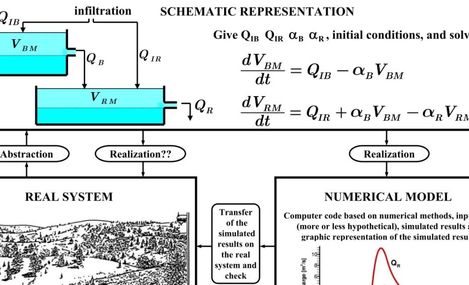
Abstraction Realization?? Realization Transfer of the simulated results on the real system and check

REAL SYSTEM NUMERICAL MODEL

SCHEMATIC REPRESENTATION

Computer code based on numerical methods, input data (more or less hypothetical), simulated results and

graphic representation of the simulated results

Representation of the principal problems in modeling groundwaterflow

R Q IB Q infiltration B Q QI R R M V B M V BM IB B BM dV Q V dt = −α RM IR B BM R RM dV Q V V dt = +α −α

Depending on the problem to solve,

the same real system

may be

represented by very different schematic

representations

We are free to invent any inevitably hypothetical and schematic representation of the real system, which helps to solve a problem

(this a question of inspiration)

But then we have to:

1. Deduce the verifiable consequences of the assumed hypotheses

2. Check the consistency of the schematic representation in a larger theoretical framework (do learn physics and some math!)

3. Check by direct or indirect experimental methods whether the real system may (or may not) be considered as a realization of the proposed scheme (do not forget the field work!)

Transfer of the simulated results onto the real system

Strictly speaking,

the simulated results are not "valid" but in the

highly simplified numerical model

. Their meaningful transfer onto the

real system requires that simplifying assumptions and

uncertainties on

the data explicitly do appear as uncertainties on the results

. This could

help to avoid such ridiculous situations as trying to simulate observed

piezometric

heads to within a few centimeters, even though the

simplified hydraulic conductivity field in the model "ignores" the

strong local heterogeneities existing in the real system.

The transfer is possible

if both the numerical model and the real

system may be considered as being

, to some extent and from a certain

point of view,

the realizations of the same schematic representation.

The central role played by the schematic representation might seem

surprising, but it is the only thing we really know, because we have

created it.

Modelling is not just curve fitting!!

FOR A GOOD MATHEMATICAL MODEL IT IS

NOT ENOUGH TO WORK WELL

IT MUST WORK WELL FOR THE RIGHT

REASONS!!

What are the « right reasons » a model should respect when simulating flow and transport in karst aquifers?

The DUALITY of karst (effect on permeability, infiltration, discharge) The NESTED STRUCTURE OF DISCONTINUITIES with « meshes » of different order of magnitudes.

The SCALE EFFECT on the HYDRAULIC CONDUCTIVITY The typical KARSTIC HYDROGRAPHS of karst springs

« DUALITY » OF KARST spring epikarst Groundwater level Discharge level

The behaviour of the whole sys-tem is determined by this duality: groundwater level, flow velocities, residence times, head distribution, spring hydrograph, chemistry, etc.

PERMEABILITY

INFILTRATION

DISCHARGE

1 High permeabilitykarsticnetwork « immersed»in 2 Lowpermeabilityfractured rock volumes

1 High intensity(« concentrated») input intothe karstic network (dolines, drainage in the epikarst zone)

2 Low_{lowpermeability}intensity(«diffuse_fractured») percolation through_volumes the

1 2

« Concentrated »from the channelnetwork at karst springs « Diffuse »from the lowpermeabilityvolumes

Scale effect on the hydraulic conductivity

Analysis of a single flood event

How to characterize the depletion (the baseflow recession) curve? How to forecast the spring discharge during drought?

How to characterize the entire falling limb? How to simulate the whole flood event?

0

( )

V t

=

V

e

( )

Q t

=

Q

e

Basics for the “global” models (2)

h _V Q Emptying of a reservoir: d V Q = − _{d t} Hypotheses

volume V is proportionalto h and discharge Q isproportional to a power of h ( V) n Q = KV / Q V α = and we have 0 n dV _KV dt + = for emptying If n=1, the recession of Q is exponential:

dV _dt

V = −α and the integralgives

In a diagram ln Q versus t the exponential part of the recession hydrograph appears as a straight line. If we know two points (Q₁, t₁) and (Q₂, t₂) on the exponential part, we can determine α by:

1

2 1 2

1 _lnQ

t t Q α = ₋

The hydrographQ(t) and α allow to estimatethe volume V by V(t)=Q(t) / α. Caution if Q is given in [m3_{/s] and α is given in [1/day]: 1 day = 86400 seconds.}

Discharge [m3_/s] Time [days] 01 Q 02

Q

Q

( )

Q t

=

Q

e

+

Q

e

+

Q

e

Hydrograph separation in 3 exponentials

R Q infiltration B

Q

Q

Q

V

V

α

α

dV

Q

V

dt

=

−

α

dV

Q

V

V

dt

=

+

α

−

α

Basics for the “global” models (4)

R Q = spring discharge B Q = baseflow component B

α

α

= recession coefficient for the slow reservoir

IB

Q _{= diffuse infiltration into}

the slow reservoir

IR

Q = direct infiltration into the rapid reservoir

BM

V = “mobile”volume of the slow reservoir

RM

V = “mobile”volume of the rapid reservoir

Spring hydrographs obtained by the double-reservoir model: effect of the form of input functions on the hydrographs Rectangular input Triangular input infiltration time [hr] α_D= 2.0 (rapid res.) α_B= 0.3 (slow reser.) i i

If you can avoid, do not use rectangular input functions

Observe the 2 inflexion points “i” on the curve Q_D2 obtained by the triangular input function. The first inflexion point is at 6 hr (infiltration has its maximum value) and the second is at 24 hr (the infiltration is ceased).

Observing the inflexion points on real spring hydrographs would perhaps allow to make a guess on the real input function.

R Q infiltration B

Q

Q

Q

V

V

α

α

dV

Q

V

dt

=

−

α

dV

Q

V

V

dt

=

+

α

−

α

V

C

C

α

:

B

α

:

IB

Q diffuse infiltration into the slow reservoir

:

IR

Q direct infiltration into the rapid reservoir

:

BM

V “mobile”volume of the slow reservoir

:

RM

V “mobile”volume of the rapid reservoir

:

RF

V “fixed” volume of the rapid reservoir : B C concentration in baseflow : R C concentration in spring : IR

C concentration in direct input

(

)

(

)

(

)

(

)

dC

C

C

C

C

Q

Q

dt

V

V

V

V

−

−

=

₊

+

₊

Basics for the “global” models (7): dilution effect at the spring

Observe that “old water” component and hydrodyna-mic baseflow are two diffe-rent concepts!!! Do not equate “old water” to “base-flow”!!

DISTRIBUTIVE MODELS

In the distributive models the flow problem is solved in a (generally great) number of “discrete” points (“nodes” or nodal points) which allow to interpolate the results over the whole region under consideration. The two most common techniques are represented by the Finite Difference models and by the Finite Element models. In both cases the exact, but unknown solution of the governing partial differential equation will be approximated by a simpler function of known type in the finite difference cells or over the finite elements (for example, constant head value in the cells and linear, quadratic or cubic function over the finite elements) which allow to obtain a (generally linear) equation for each node of the model. The system of simultaneous linear equations is then solved by iterative or direct numerical methods. Data necessary for the distributive models and how to obtain them?

Hydraulic Head and Flow Fields

Flow equations, Models

Hydraulic Properties

3-D fields of hydraulic conductivity [K], storage

Ss , porosity me , etc.

Boundary Conditions

Heads, source terms, river/groundwater inter-

actions, etc.

Void Geometry

Orientation, density, ope- ning, extension, connec-

tivity, etc.

Geol. Discontinuities

Fractures, faults, karst channels, pores, etc.

Geological (genetic) Factors

Lithology, sedimentary structures, mechanical properties of the rocks, small and large scale deformations, stress and

strain history, etc.

Geomorphological and bio-climatic

factors

Relief, river network, soils, vegetation, hydrometeoro- logy, human intervention, climate changes, karst, etc.

"s hort c irc uit" transformation transformation transformation transformation extrapolation extrapolation extrapolation extrapolation extrapolation extrapolation Measured values extrapolation Measured values Measured values observations Measured values Measured values Measured values observations Measured values observations relations relations relations relations

Problems related to the indirect reconstruction of the hydraulicparameter fields and boundary conditions (interpolation or extrapolation of the measured values or observations

Block-centered Grid System

Point-centered Grid System

y

Δ

y

Δ

x

Δ

x

Δ

Note that in each cell the hydraulic head is considered as being constant!! If possible, do not use Finite Diffe-rence models to simulate karst aquifers: Finite Element models are better for solving karst problems.

Extended

example: Numerical simulation of

the aquifer at Mammoth Cave (MODFLOW)

(Steven Worthington, unpublished data)

Map of the Mammoth Cave area

(Steven Worthington)

550 km length!

Model 1: homogeneous Equivalent Porous

Medium (EPM)

(Steven Worthington)

Data for calibration

•

Heads in wells

•

Hydraulic conductivity

from well tests

Matrix 2 x10-11 _m/s

Slug tests (geo. mean) 6 x 10-6 _m/s

Slug test (arith. mean) 3 x 10-5 _m/s

Pumping tests 3 x 10-4 _m/s

Results: groundwater contour lines

48 wells

mean absolute error = 12 m

Results: Simulated tracer paths

54 tracer injection locations

Actual tracer paths

from 54 points to 3 springs

Model 2: EPM with ‘conduit cells’

•

Aquifer has integrated conduit network

•

Can be simulated with high conductivity cells

•

Useful data for calibration

–

1) Heads in wells

–

2) Hydraulic conductivity from well tests

–

3) Heads and discharge in conduits

Results: groundwater contour lines

mean absolute error = 4 m

Results: Simulated tracer paths

all 54 tracer paths

go to correct spring

Double Continuum Approach

(DC)

8

6

EXAMPLE OF FINITE ELEMENT MODEL

Bi-quadratic function over an 8-node 2-D element (blue) circles: nodal points on the 2-D element

Examples of quadratic functions over 2-D quadratic finite

Areuse spring gallery threshold of Bois de l’Halle regularized discharge Brévine syncline

2-D Finite Element model of the Areuse spring basin

thick lines: high conductivity 1-D elements simulating the karst channels

Areuse spring gallery

regularized Example of regularization of the Areuse river

Hydraulic conductivity and efficient porosity values for various networks of fractures (left) and intersections of fractures or karst

channels (right)

K1 K3

Effect of the density of the high conductivity drainage network on the recession curve of karst springs.

The “Faraday-cage” effect of epikarst

The recharge mechanisms of the huge low permeability volumes may have important practical consequences on the groundwater management problems. The theoretical model studies suggest, that a well developed epikarst layer enhancing the concentrated infiltration into the high conductivity karst channel network will short-circuit the low conductivity volumes and will play the role of a Faraday-cage with respect to the main aquifer.

Depending on the importance of this Faraday-cage effect, the recharge of the low conductivity volumes could be much smaller than in case of pure diffuse infiltration, with important consequences on the groundwater management problems. In the deep syncline configuration the inversion of gradients will always contribute to recharging the low conductivity volumes “from the interior”, but in the shallow karst configuration the short-circuit of the low permeability volumes might be almost total.