Modeling the transition to turbulence in plane Couette flow

(1)

HAL Id: pastel-00675068

https://pastel.archives-ouvertes.fr/pastel-00675068

Submitted on 28 Feb 2012

HAL is a multi-disciplinary open access

archive for the deposit and dissemination of sci-entific research documents, whether they are pub-lished or not. The documents may come from teaching and research institutions in France or abroad, or from public or private research centers.

L’archive ouverte pluridisciplinaire HAL, est destinée au dépôt et à la diffusion de documents scientifiques de niveau recherche, publiés ou non, émanant des établissements d’enseignement et de recherche français ou étrangers, des laboratoires publics ou privés.

Modeling the transition to turbulence in plane Couette

flow

Maher Lagha

To cite this version:

Maher Lagha. Modeling the transition to turbulence in plane Couette flow. Mechanics of the fluids [physics.class-ph]. Ecole Polytechnique X, 2006. English. �pastel-00675068�

(2)

´

Ecole Polytechnique

Laboratoire d’Hydrodynamique

Thèse présentée pour obtenir le grade de

DOCTEUR DE L’´

ECOLE POLYTECHNIQUE

Spécialité : Mécanique

par

Maher LAGHA

Modeling the transition to turbulence

in plane Couette flow

soutenue le 8 d´ecembre 2006 devant le jury compos´e de :

M. Patrice LE GAL Examinateur IRPHE, Marseille

M. Dwight BARKLEY Rapporteur Warwick University, Grande-Bretagne

M. Fran¸cois DAVIAUD Examinateur SPEC-CEA, Saclay

M. Bruno ECKHARDT Rapporteur Philipps-Universitat, Marburg, Allemagne

M. Paul MANNEVEILLE Directeur de th`ese LadHyX, Ecole Polytechnique

(3)

(4)

Foreword

The transition to turbulence in shear flows still leaves open several problems of great practical importance. This thesis is the continuation of the work of the Saclay group in this field. Their main focus was the investigation of the growth of a finite amplitude perturbation introduced in the laminar plane Couette flow (pCf), a shear flow between two parallel plates. When the control parameter exceeds a certain threshold, this perturbation is self-sustained and gives rise to a turbulent region, called a spot. Their study raised many questions and in this thesis we focus on few of them: How do this turbulent region sustains itself? What is the mechanism that spreads this turbulent region into laminar domain? The turbulent domain looks separated from the laminar domain by a sharp boundary, but is the flow outside this spot laminar? Once all the domain has become turbulent, how is the distribution of the durations needed to relax towards laminar state when the control parameter is decreased below the threshold?

To bring some elements of answer to these questions, we have derived a model of pCf in terms of partial differential equations (PDEs) using the Galerkin method. In this derivation, we used an assumption based on the experimental observation of the Saclay group, which is the coherence of the observed structures between the two plates, which permits us to consider few cross-stream modes. This simplification makes the identification of involved physical mechanisms eas-ier than using simulations of the full dynamic equations. This kind of model allow us to approach the problem of spot propagation that requires explicit space dependence (spatiotemporal chaos), by contrast with models in terms of ordi-nary differential equations, obtained by frozen this spatial dependence (temporal chaos).

The outline of the manuscript is as follows. In chapter I, we review some ex-periments and results from the literature related to the questions under scrutiny: The first part of this chapter concerns the recent studies of the distributions of the transient lifetimes. The second part is dedicated to the spot spreading mech-anisms and more generally to the coexistence between turbulent/laminar state. The last part concerns the self-sustainment of the turbulent state.

Then, in chapter II, the derivation of the model is detailed. The numeri-cal method and some results are presented in chapter III. We show that this model reproduces the globally sub-criticality of pCf and that the global stability

(5)

4

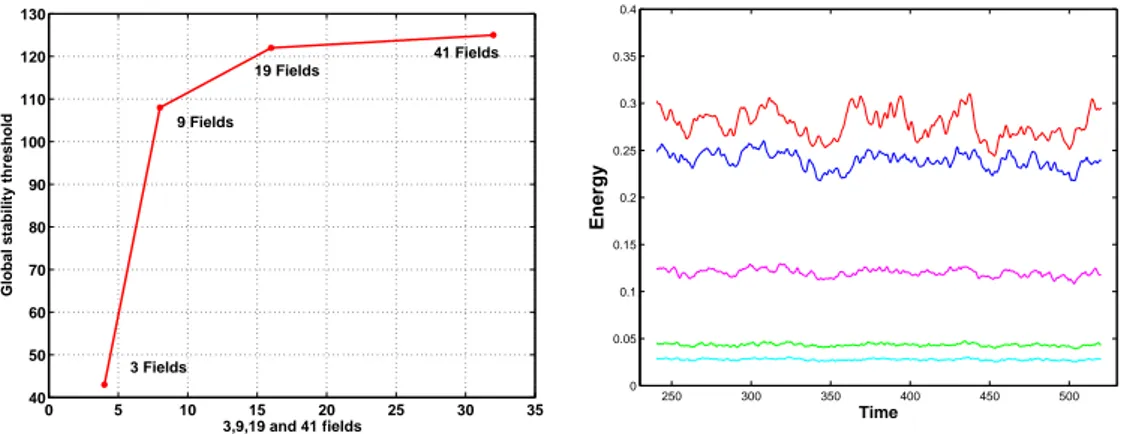
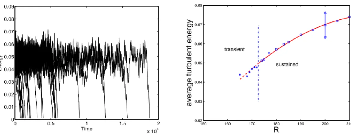
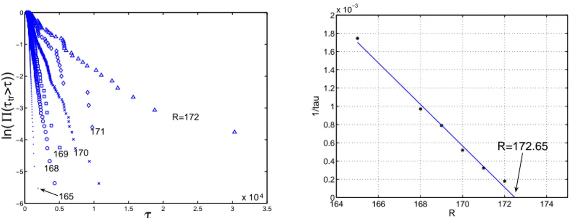
threshold (Rg) using this model is found to be a factor 2 less than the one in the experiences. The extensivity of the turbulent state is also addressed. Then, the study of the distributions of the transient lifetimes shows the same behavior as in the experiments of the Saclay group: exponential decay of the duration of the

transients and a divergence of the mean value of these duration in 1/(Rg − R),

where R is the Reynolds number.

In chapter IV, we are interested by the self-sustainment of the turbulence inside a growing turbulent spot as well as in a fully turbulent domain. A brief survey of the work in the literature shows that the key question is about the generation of streamwise vortices. After analyzing the different terms in the streamwise vorticity equation, we find that the tilting term of the wall-normal vorticity into streamwise direction is the dominant term, in accordance with the other studies. However the tilting term of spanwise vorticity into streamwise di-rection is not negligible. By analyzing each term contributing to the generation of streamwise vorticity in physical space and tracking the evolution of this vorticity into streamwise vortices in time, we discovered a simple process for streamwise vortices generation where the flow field (U0, W0) related to the streaks (repre-sented by the velocity component U0 in our model and where ∂xU0+ ∂zW0 = 0) plays a crucial role. This process can be summarized as follows: a spanwise vor-tex is deformed by this flow and gives a crescent vorvor-tex where its legs are two counter-rotating vortices. They regenerate the streaks by the lift-up effect. We find that the streamwise vortices are generated in regions where a positive streak encounters a negative streak and results in a stagnation-like point, i.e., where

∂xU0 ≤ 0 and U0 ≈ 0. Then, we derive a 1D-model in terms of four PDEs,

show-ing the generation of streamwise vortices from spanwise vortices. The last part of this chapter is concerned with the generation of spanwise vortices. Under the action of the flow field (U0, W0), a localized region of streamwise velocity correc-tion, represented in the model by U1 ≤ 0, is stretched in the spanwise direction, under the action of W0 (where ∂zW0 =−∂xU0 ≥ 0). To this z-elongated region, a vertical velocity is generated by the pressure to ensure the continuity

equa-tion. This vertical velocity and the z-elongated region of U1 form the spanwise

vortex. Finally, by piecing together the mechanisms described in this chapter, a self-sustained process for wall-turbulence is proposed.

In chapter V, we focus on the spot spreading mechanism. First we analyse the coherent structures on the border between the laminar and turbulent regions. This reveals us the existence of many vortices with cross-stream axis extending all over the gap. The streamwise velocity component of these vortices is the streak

(U0). The vortices move parallel to the plates and we show that the origin of

this motion is essentially due to the action of each vortex on the other. During their motions, these dipoles carry the other perturbation components such as the streamwise and spanwise vortices. This is the spreading mechanism. A simple 1D-model in terms of 8-PDEs is derived to corroborate it.

(6)

5

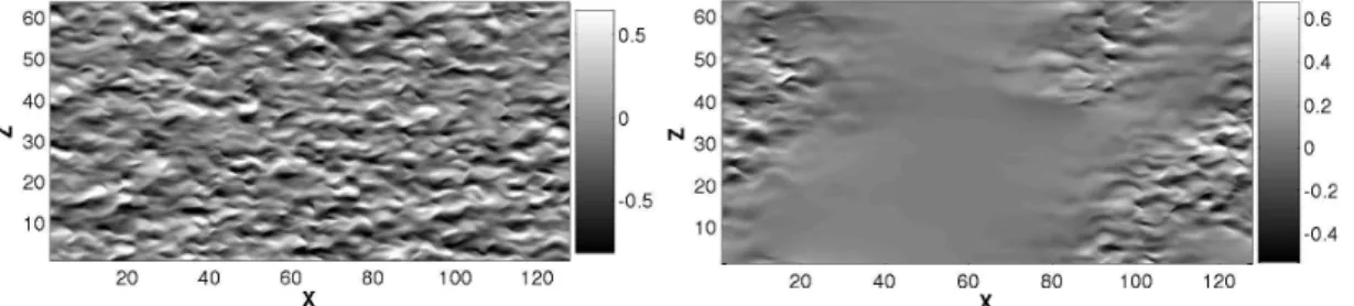
a spot, our numerical results show the development of large scale flow, extending over the whole gap, characterized by streamwise inflow and spanwise outflow, giving it a quadrupolar shape. The spot is associated to a region where the

streamwise velocity correction (U1) is dominantly opposed to the base flow, as

seen by filtering out small-scale fluctuations. The origin of the quadrupole-like flow is traced back to the shearing of this negative correction by the base flow, whereas the correction itself is generated by the appropriate component of the local average of the small-scale Reynolds stresses (streaks and streamwise vor-tices).

Chapter VII is our concluding chapter. We summarize the work of this thesis and we present some questions that we intend to examine by going beyond the case of pCf and considering other wall flows experiencing a similar transition to turbulence, such as plane Poiseuille flow and Taylor-Couette flow in narrow gap.

(7)

(8)

Chapter 1 Introduction

The transition to turbulence in shear flows close to a solid wall still leaves open several problems of great practical importance. This situation arises because linear stability analysis is less fruitful for stable systems in which transient al-gebraic energy growth may become relevant than when exponentially growing modes are present. As a matter of fact, things are easier to understand in the case of supercritical instabilities —especially in closed-flow configurations, e.g. Rayleigh–B´enard convection and the Taylor–Couette instability— for which the classical tools of weakly nonlinear analysis are available. The situation is indeed delicate to handle in the case of a discontinuous transition marked by a competi-tion between solucompeti-tions arising from linear instability modes and other nonlinear solutions, i.e. in the globally subcritical case (Dauchot & Manneville (1997) (21)). A classical example is the plane Poiseuille flow —the flow between two parallel plates driven by a pressure gradient— which is linearly unstable only beyond

some high Reynolds number Rc (Orszag (1971) (74)) while turbulent spots, i.e.

patches of turbulent flow scattered amidst laminar flow and separated from it by well defined fronts, can develop in the flow for R as low as about Rc/4 (Carlson et. al.(1982) (16)).

The situation is even worse for the plane Couette flow (pCf in the following) — the simple shear flow driven by two plates moving parallel to each other, Fig. 1.1—

which is stable for all R, hence Rc=∞ (Romanov (1973) (84)), but experiences

a direct transition to turbulence at moderate values of R ((61; 98; 22)). Standard modal and non-modal linear theory, as reviewed e.g. in Schmid & Henningson (2001) (88), is of little help to understand the main problem alluded to above, namely the nonlinear coexistence in physical space of these different solutions testified by the existence of turbulent spots.

A detailed understanding of this transition to turbulence (globally subcrit-ical) via turbulent spots nucleation and growth, relies on (i) an understanding of microscopic processes such as the self-sustainment of turbulence and (ii) the mechanism by which it propagates into the laminar domain. In the other hand, some studies have been devoted to the transition from turbulent to laminar flow.

(13)

4 Introduction

Figure 1.1: Left: Experimental set-up for plane Couette flow, used by the Saclay Group. Right: Laminar regime with linear velocity profile. Adapted from Man-neville (2004) (64).

They were motivated by the determination of the stability threshold (usually noted Rg) and also to investigate the behavior of the transient lifetimes near this threshold.

We present some related works in_{§1.1. The development and growth of the}

spot is presented in§1.2. Some studies concerning the spreading mechanisms are

summarized in _{§1.3. The process related to the self-sustainment of turbulence}

(inside the spot) is discussed in _{§1.4. Throughout this chapter, we use a common}

coordinate system with x in the streamwise direction, y along the normal to the wall and z in the spanwise direction. The base flow is U and the fluctuations are u, v, w. Most of the studies that we have found in the literature and which we present in this chapter, are related to the turbulent boundary layer flow. Few are concerned with the plane Couette or Poiseuille flow. The relevance of those studies in understanding transitional flow especially pCf is justified by the fact that turbulent flows in pipes, channels and boundary layers have some common features, investigated below.

1.1 Transient lifetimes

1.1.1 Introduction

As it seems to be strange, the study of the transition from turbulent to lam-inar state might bring some valuable elements to understand the transition to turbulence itself. For example, this approach permits one to determine, with a reasonable accuracy, the stability threshold (Rg).

Determining the distribution of the durations needed to relax from turbulent state towards laminar state when the control parameter is decreased below the threshold, was the aim of some studies. We summarize here some of them and outline a few hints for our own study.

(14)

1.1 Transient lifetimes 5

1.1.2 Numerical and experimental studies

In phase space, we can consider that the laminar state is a fixed point. Since the plane Couette flow is linearly stable, all points in the neighborhood of this fixed point evolve towards it. The ensemble of these points form the basin of attraction of the laminar state. Far from this basin, there is the turbulent state with its complicated structure:an initial condition can remain turbulent while another one very close to it can relaminarize. Such a structure is known, in dynamical systems theory, as a chaotic saddle.

Some insight in this saddle can be obtained by studying the distribution of lifetimes of turbulent transients. Many researchers went this way, using both ex-perimental and numerical methods, to collect a large number of lifetimes, for pipe flow and plane Couette flow. We will not describe the methods used in analyzing the transition and determining the lifetimes (usually based on the determination of the point in time where the energy drops below a threshold). For a fixed

Reynolds number below the threshold Rg, the probability to stay turbulent for

a duration of t = δt1 is less than the probability to stay turbulent for δt2 ≤ δt1.

Theory of dynamical systems predicts a probability Π _{∝ exp −t/τ(R), where τ}

is a characteristic decay time (also the lifetime). This exponential behavior was obtained, among others, by Darbyshire & Mullin (1995) (20) for pipe flow as in pCf experiments by Bottin & Chat´e (1998)(11). The natural question that arises is how τ depends on R.

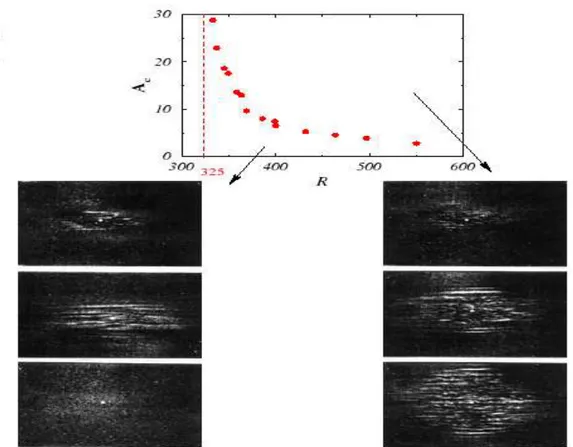
For pCf, lifetimes have been measured experimentally by Bottin & Chat´e

(1998) (11) in a large box with streamwise and spanwise lengths Lx = 190 and

Lz = 35. They observed that τ increased continuously with R, suggesting a

divergence at some finite value of R. By fitting their data, they concluded that the best fit for τ is τ ∝ (Rg − R)−1, where Rg = 323± 2 is the global stability threshold.

Peixinho & Mullin (2006) (78) run experiments in pipe flow and have

ob-tained an exponential distribution of lifetimes. They have shown that τ _∝

(Rc− R)−1±0.02, where Rc = 1750± 10 is the critical Reynolds number. They

pointed out that in dynamical systems theory, this behavior of τ is a generic feature associated with transient behavior where an attractor loses stability at a crisis.

Hof et. al. (2006) (45) presented new experimental data showing that the lifetime does not diverge but rather increases exponentially with R. This has been achieved by increasing the observations times (up to two order of magnitude) for turbulent transient in a long pipe flow (30 m). They showed that τ can

be best approximated by τ−1 _{= exp (a + bR) where a and b are two constants}

determined from the fit. By means of numerical simulations, they confirm the exponential fitting for τ (observations time around 3000 and the shorter extend of the numerical pipe). They proposed that reanalyzing some distributions found in the literature by subtracting a time t0 to t in the expression of the probability

(15)

6 Introduction

Π can substitute the exponential behavior of τ−1 _{by its linear scaling.}

As a conclusion, determining the behavior of the transient lifetimes remains a controversial issue.

1.2 Turbulent spots

1.2.1 Introduction

Turbulent spot is commonly used to describe a turbulent region sitting in a lam-inar flow. During the transition process from lamlam-inar to turbulent flow, small turbulent spots develop. They can be considered as the “building block” of a space-time chaos. In a natural transition (as opposed to triggered), the first ap-pearance of turbulent spots determines the start of transition location and the subsequent growth of the spots leads to the turbulent flow. The main character-istic of the transition is the coexistence of the two states turbulent and laminar. Emmons (1951) (31) first recognized the intermittent nature of transitional flow and the role of the turbulent spots in the transition process. Pomeau (1986)(81) studied this transition and conjectured that it could be represented by a contamination process model, i.e., a model in which a laminar site becomes turbulent with some probability: the growth of the turbulent region results purely from a stochastic process (see _{§1.3 below).}

Such a transition to turbulence has been studied recently. Many new tech-niques, as high-resolved direct numerical simulations (DNS) or stereo particle image velocimetry (PIV), have been employed to track the growth and move-ment of the spots. New phenomena have been observed and would lead to better understanding of spots dynamics. In the next section, some of these phenomena are presented.

1.2.2 Characteristics of turbulent spots

Attempts to investigate the interior structure of a turbulent spot and, in partic-ular, the mechanisms involved in its development, have been undertaken recently by many researches.Only some studies are presented here.

Lundbladh & Johansson (1991) (61) studied the development of turbulent spots in pCf by means of direct numerical simulations (DNS). At that time, in 1991, due to the absence of experiments for this kind of study, their results represented a prediction of the physical situation. They found that spots were

sustained for Reynolds numbers above approximately Rg ∼ 375 and that their

shape was elliptical with a streamwise elongation that was more accentuated for

high Reynolds numbers. For R = 300 < Rg, the energy of the disturbed region

decayed. The u-disturbance decayed more slowly, but at large times the remaining u-disturbance consisted merely of long longitudinal streaks of alternating low and

(16)

1.2 Turbulent spots 7

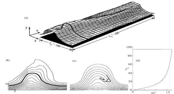
Figure 1.2: From (61). The isocontours of (a)-u,(b)-v,(c)-w velocity in the (x, z)-plane for y = 0. The solid contours represent positive value and the dashed contours represent negative values. There is an inflow toward the spot in the streamwise direction (represented by u) and an outflow from the spot in the spanwise direction (represented by w). The remaining distribution of v in this figure highlight a positive region at the leading edge of the spot and a negative region in its tail. Both regions are elongated in the spanwise direction.

high velocity, dominated by one specific spanwise wavelength. At R = 375 the turbulence was seen to be self-sustained as the region grew. From an analysis of the data, they found that the velocity field outside the spot was essentially two-dimensional in that it lacked a significant vertical component. Spatially filtered mean values were obtained by use of a Gaussian low-pass filter in wavenumber space. Various values of the filter length-scale were tested. The results were found to be rather insensitive to the choice of this length-scale. Figure 1.2 shows the averaged u, v, and w fields at the mid-plane y = 0. The modification of the external flow standed out in a clear way as the turbulent fluctuations of the interior were filtered out. They have seen that the modified external flow is totally dominated by the horizontal components and that there is a motion out from the

(17)

8 Introduction

Figure 1.3: Experiments on turbulent spots by the Saclay group (1998). If the amplitude of the initial perturbation is sufficiently high, it gives rise to a growing turbulent spot, otherwise, it decays.

spot near the midpoint x = 0, contrasted with motion towards the spot at the leading and trailing parts (as we have found with our models). Notice that this motion shows a quadrupolar pattern outside the spot, which was not mentioned explicitly in the paper of (61). Finally, they found that spanwise growth increased with increasing R for low values, but leveled off to a constant rate at high R. As we will see later on, the investigations of Schumacher & Eckhardt (2001)(91) have shown the existence of the quadrupolar flow.

Dauchot & Daviaud(1994) (22) reported a detailed study of the transition to turbulence in pCf. Externally applied perturbations that trigger turbulent spots were made by injecting turbulent jets into the laminar flow. As shown in Fig. 1.3, they found that if the amplitude of the initial perturbation is sufficiently high, it gives rise to a growing turbulent spot, otherwise, it decays. All perturbations

are observed to decay below R = Ru ≈ 310 so that the flow rapidly returns to

(18)

1.3 Spreading mechanisms 9

Figure 1.4: Some results of the Saclay group (1998). Left: Photograph of the gap in the (y, z)-plane using Pyroceram particles. It shows the cross section of vortical structures in the (y, z) plane at R = 380 as indicated by the arrows. This is a cross section of the streamwise vortices that have been observed to pervade the spot (right panel). The presence of these structures correlates well with the streaks in the (x, y) plane visualizations using Iriodin particles and shows that the streaks and streamwise vortices are correlated.

plate velocity, h is the half-gap between the plates and ν the kinematic viscosity of the fluid). Between Ru and Rg ≈ 325, localized finite-amplitude perturbations generate turbulent spots with finite lifetimes. These lifetimes increase as Rg is approached from below, while beyond this value, most of the spots no longer decay but on the contrary invade the system. A regime of uniform featureless

turbulence is eventually obtained beyond Rt = 415.

In the other hand, turbulent spots may form a variety of temporal shapes which can be distinguished easily because of a sharp laminar/turbulent interface. As these spots evolve, they grow, split and merge. The streakiness of the spot was visible, as clearly shown in Fig. 1.4.

Hegseth (1996) (38) carried out and experimental study of the coexistence of laminar flow and turbulent spots in pCf. He observed vortical structures in the (z, y) plane as shown in Fig. 1.4. The circular structures in the figure could be interpreted as cross sections of streamwise vortices that pervaded these spots. Their temporal behavior was quite complex and included events such as vortex creation, destruction and motion. These vortices almost filled the entire gap.

1.3 Spreading mechanisms

Roughly speaking, a complex spatiotemporal behavior that involves two phases (a simple one, that describes a so-called laminar state and a complex one, that

(19)

10 Introduction

has been called turbulent state) is called spatiotemporal intermittency. It denotes a complex dynamical behavior which is observed in spatially extended physical systems.

The two states are separated by a front and the laminar state disappears through the propagation of this front. Two types of front have been defined in the literature: pulled and pushed.

In a complete review by Van Saarloos (2003)(105), the name pulled front comes from the fact that such a front is being “pulled along” by the leading edge of the front, the region where the dynamics of the front is governed by the equations obtained by linearizing about the unstable state. In this way of thinking, a pushed front is being pushed from behind by the nonlinear region.

From the theoretical side, little is known about the question of coexis-tence between laminar flow and turbulence and the possible mechanisms of (pulled/pushed) front propagation leading to the spreading of turbulent spot.

This question was discussed by Pomeau (1986)(81) from a fully abstract point of view as a nucleation problem in terms of first-order phase transition. He argued that when one of the competing states was chaotic, the competition could be understood in terms of a stochastic contamination process in the same class as directed percolation. In fact, directed percolation (DP) is the common name for spreading processes with active (“live”) sites and an absorbing (“dead”) state. Note that DP is a purely statistical process with no a priori dynamics; at each time step, a site can become alive with probability p, if and only if at least

one of its neighbors was alive at the previous time step. For p _{≈ 0 the process}

rapidly terminates whereas for p _{≈ 1, the live sites spread without limit. The}

concrete connection between DP and subcritical transition to spatio-temporal intermittency in hydrodynamic context, is still an open question.

Based on experiments in boundary layers flows, Gad-El-Hak et. al. (1981)(33) proposed a mechanism called “growth by destabilization”. If the mean transport velocity of the spot is lower than the mean velocity of the surrounding flow, the spot acts as a blockage and the laminar flow field outside the spot is accelerated. The linear stability of the profile maybe be lost and the growth of infinitesimal perturbations occur.

Dauchot & Daviaud (1994)(22) discussed this mechanism in an experimental study. They found velocity profiles indicating that the flow is accelerated outside the spot. They also envisioned another mechanism related to the transient growth of perturbations. But a direct demonstration of both mechanisms has not yet appeared.

Spanwise spreading of the turbulent spot was investigated by Schumacher & Eckhardt (2001) (91). They performed direct numerical simulations of Navier-Stokes equations for plane Couette flow with free-slip boundary conditions and added a bulk force to drive the flow. They found that the front advances at a rather well-defined speed in the spanwise direction and that the presence of the turbulent spot gives rise to a large-scale spanwise outflow.

(20)

1.4 Self-sustainment of wall-turbulence 11

They defined vf, the velocity of the turbulent spanwise-advancing front. They

showed that this velocity vf was different from the large-scale spanwise outflow

velocity but they conjectured that this outflow had profound consequences for the spreading of the spot. They also analyzed the linear spreading velocity v⋆ _by linearizing the flow equations about a laminar state viewed as a sum of the base flow and this large-scale outflow, using an Orr-Sommerfeld equation. The mea-sured front speeds in the numerical simulations were about a factor 10 larger that

the value of v⋆ _{obtained this way, leaving no doubt that the spanwise spreading}

of the turbulent spot is not governed by a linear mechanism.

The question of which mechanism is involved in spot spreading (in shear flows in general) is to a large extent open. We were motivated to study the spot spreading within our model.

1.4 Self-sustainment of wall-turbulence

In this section, some studies related to the self-sustainment of wall-turbulence are presented. Most of the investigations in this field were concerned with boundary layer, few with pCf or Poiseuille plane flow. We have decided to present some of them, since they can give us valuable hints to our study.

1.4.1 Definition of coherent structures

It is natural that in the aim to understand the wall turbulence, we use flow patterns as building blocks. The purpose of this section is to define and describe these elements in a simple way. These elements are called coherent structures, noted as “CS”. Townsend in 1959 gave one of the first definition to coherent structures: “a flow pattern which is of finite size, mechanically coherent and resistant to disintegration”. One of the first CS was proposed by Theodorsen in 1951. He imagined that a vortical element, with its spatial structure looks like a horseshoe (Fig. 1.5), arose from the wall to transport fluid (v _{6= 0). This} horseshoe vortex has two legs located near the wall, forming two counter-rotating streamwise vortices, another important CS in wall-turbulence. He introduced this concept, from a phenomenological point of view, to explain and to link all the observed turbulent flow events (defined later on).

Streaks were also among the first and most important elements identified in the early experiments. They were observed near the wall. In a review article, Corrsin (1955)(17) discussed some experiments concerning the behavior of dyed fluid being replaced by clear fluid in a tube flow. He stated:“The significant property seems to be the strong orientation into streamwise filaments of the residual dye. Presumably this indicates a predominance of axial vorticity near the wall, sweeping the dyed wall fluid into these long narrow stripes.” The existence of many streamwise vortices near the wall, lifting up near-wall fluid, is a possible

(21)

12 Introduction

Figure 1.5: Different parts of a hairpin vortex (Theodorsen, 1951). A vortical element, with its spatial structure looks like a horseshoe, arose from the wall to

transport fluid (v _{6= 0) and produces Reynolds stress (−uv 6= 0).}

explanation. Since the near-wall fluid has a low speed, the term “low-speed streak” is often used. On the other side of the vortex, fluid from a higher speed region is brought closer to the wall. The high-speed regions are devoid of dye because the fluid comes from region far from the wall.

The term “streak” originated from the behavior of flow visualization markers. Nowadays, we use streaky flow to describe a U (y, z) velocity profile that has an oscillation in the z-direction. As we will see later on, this streaky profile is used in stability considerations.

1.4.2 Kinetic energy production

It is of interest to look at the spatial region where turbulent kinetic energy is

pro-duced. The Reynolds-Orr equation gives turbulence production P = −huvi∂yU

where _{−huvi is one component of the (averaged) Reynolds stress. We are}

in-terested in the processes that make essential contributions to P , i.e., why there

is, somewhere in space, a correlation between u and v such that −uv is positive

(since ∂yU > 0) rather than negative.

When flow is ejected from the wall, by a vertical velocity v > 0, it cre-ates low speed streaks, u < 0, since the streamwise velocity at this location is

now 0 < U (y) + u < U (y). Hence, this ejection event makes a positive _−uv

contribution to the Reynolds stress and is defined as Q2 event. Similarly, any

coherent event producing a Q4 contribution is frequently called a “sweep”. A

high speed streamwise-flow comes close to the wall by negative vertical velocity v. It generates positive streaks since near the wall, the streamwise velocity is now U (y) + u > U (y), i.e. u > 0. Hence, this sweep event makes also a positive −uv

(22)

1.5 Characteristics of self-sustaining

mechanisms 13

contribution to the Reynolds stress. A general concept is that the Q2 and Q4

events occur on each side of a streamwise vortex and hence those regions make a significant contribution to the energy production. For this reason, elucidating the dynamics of the streamwise vortices is crucial in understanding the production of turbulence.

1.5 Characteristics of self-sustaining

mechanisms

To summarize the previous sections, we state that where Reynolds stress −uv

is positive, kinetic energy is produced. Since the key structure involved in such production are the streamwise vortices, which appear and disappear, we may understand that there is a cycle governing the generation of such vortices. The occurrence of this cycle guarantees the self-sustainment of turbulence. The cycle can be envisioned as follows: many different structures constitute the skeleton of this cycle and they are linked together by some mechanisms. The main effort to provide is to establish the cause-and-effect relationship between these structures and the mechanisms behind their generations. Many studies are concerned with identifying the structures, based on experimental or DNS data. A few others focus on the mechanisms leading from one structure to another (actually there are very few mechanisms, the well known is the lift-up, by which, the streamwise vortices generate the streaks).

A self-sustaining cycle has several characteristics. The first might be the time scale of the repetition of events. The time interval between the coherent structures should be the same, or at least comparable between the cycles. Another important characteristic is the spatial features of the coherent structures. It is not clear that the generated streaks have the same amplitude (or strength) and the same spanwise width as the previous streaks. Same question holds for the streamwise vortices, especially if they are or not strong enough to restart the cycle.

Another characteristic concerns the nature of the process. Some of them include an instability, whereas in others, a vortex can generate another vortex. Hence, in discussing self-sustaining mechanisms, we will use two main classes (for a complete review, see Panton (1997) (76) and Panton (2001)(77)). The “parent offspring” class is defined by having a flow structure that develops in time to replicate itself without involving an instability. The second class has, during part of the cycle, a velocity profile that is unstable to small disturbances.

(23)

14 Introduction

1.6 Self-replicating mechanisms

Let us first summarize generally accepted ideas ((77)). First, there are the streaks. It is almost universally agreed that the streamwise vortices near the wall sweep low speed fluid into the low-speed streaks (lift-up mechanism). On the other side of this vortex, high-speed streaks are generated. This produces a characteristic streak velocity profile (u) with spanwise variation. Together with the vertical motion v of the streamwise vortices, Reynolds stress are produced.

Many people view the streamwise vortices as the legs of hairpin vortices (see Fig. 1.5). From this viewpoint, the self-sustaining mechanism centers on how hairpin vortices are produced given the initial situation as a fully developed tur-bulent state. Here we focus on how a hairpin vortex is generated, or springs from another hairpin vortex.

Brooke & Hanratty (1993)(15) performed computation of a channel flow and examined vorticity patterns in (y, z) planes. Viewing (y, z) planes enables one to see streamwise vortices, even if the vortex axis is not exactly in the (y, z) plane. They found that a new vortex is born at the downstream end of the parent on the down-wash side. This end is lifted from the wall and they refer to it as the detachment point. They remarked that the vorticity in the child vortex is of the opposite sign to that of the parent and that the regeneration is not influenced by outer flow events. Thus, they envisioned a regeneration process that is entirely within the inner region.

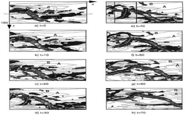
An interesting contribution is given by Heist et. al. (2000)(43). They iden-tified a new process that forms about 30 percent of the streamwise vortices. This was accomplished by examining the changes, with time, of the turbulent field obtained from a direct numerical simulation of turbulent flow in a channel. Streamwise vortices create a shear layer by pumping low momentum fluid from the wall. One or more small spanwise vortices are formed at the top of this layer. They grow in size and rotate in the direction of flow. The main focus of Heist’s paper is not on how they form but on what happens after they form. Figure 1.6 is a plan view of their DNS results. Vortex A is followed as a parent that produces vortex B. Vortex B grows in the spanwise direction and then elongates in the streamwise direction and intensifies.

Previous investigators have suggested that spanwise vortices could have a direct role in the formation of streamwise vortices. A number of investigators have argued that spanwise vortices play a key role in sustaining turbulence. Different proposals have been made to explain how this occurs. A common assumption is that spanwise vortices evolve into hairpin vortices, but the details of this process are not given (see e.g. (77)).

A common picture (among many others) about the hairpin vortex generation is presented in (76). A streamwise vortex collects fluid from near the wall and creates a low-speed streak. Next, the low-speed streak region forms an obstacle for the faster moving stream. This event takes place as long as the

(24)

stream-1.7 Instability-based mechanisms 15

Figure 1.6: Birth of vortex B and its growth and elongation. From (43).

wise vortices exist and pump more fluid into the streak area. Hence, this lifted area produces a streamwise shear, due to the impingement of the faster moving stream on it. This lifted region produces a stronger U (y) shear layer which rolls up, much like a Kelvin-Helmholtz cat’s eye, into a vortex arch or head. The vortex lines in the head extend down. As the head is convected downstream, the legs are stretched and the swirling thereby intensified. Thus, the hairpin for-mation process consists of streak lift-up, shear layer intensification, and hairpin re-formation.

1.7 Instability-based mechanisms

The class of self-sustaining processes involving instability mechanisms is now discussed. During part of the cycle, a velocity profile is unstable to infinitesimal perturbations and a linear theory is developed. The velocity profile, which must exist for sufficient time for the instability to develop, can be the base flow. A perturbation is added to it and the question is, does this disturbance grow or not. More specifically, what kinds of perturbations grow and how fast do they grow. In order to form a complete cycle, the instability should ultimately lead back to produce the initial velocity profile.

(25)

sta-16 Introduction

bility analysis. The next choice concerns the equations that are used to follow the development of the disturbance. Typical laminar flow stability analysis uses linearized equations under the assumption that they govern the initial devel-opment of infinitesimal disturbances. Furthermore, linear equations have many mathematical properties. They allow an analysis by normal modes, i.e., the eigenfunction and eigenvalues of the system. The fastest exponentially growing normal mode determines the characteristics of the most-unstable infinitesimal disturbance.

In some cases as pCf, this approach fails. However, the linearized Navier– Stokes equations are non-normal and their eigenfunction are not orthogonal. This allows certain disturbances that are composed of several normal modes to grow to large amplitudes. Factors of 1000 or more have been found. At large times the disturbance approaches the behavior of the last decaying eigenfunction. This transient growth is algebraic and for that reason this phenomenon is also called algebraic growth (as we see later on, Schoppa & Hussain used this transient growth to show that normal modes growth is not sufficient to trigger nonlinearity). Trefethen & Trefethen (1993) (100) make an analogy with vectors. Consider two almost oppositely directed basis vectors that have large amplitudes. These are normal mode components. Their resultant, the perturbation, has only a small magnitude. Then, one basis vector magnitude decreases with time while the other is unchanged. This causes the resultant perturbation to increase in amplitude. Ultimately, the behavior of the resultant perturbation follows the dominant eigenvector and decreases (stable case).

Transient growth was ignored for many years. Recently, it was realized that it could lead to profiles that, because of their large amplitude, are subject to secondary instability and or nonlinear effects. Transient growth has a history of development and a nice introductory review is in (100).

Hence, in the instability mechanism class there are many questions. They concerns the nature of the perturbations (finite or infinitesimal), the equations to be used and the approach (normal mode or transient growth). Note finally that what happens when nonlinear effects become important is another (difficult) issue.

1.7.1 Inflectional profiles

In the first flow visualization experiments, Kline & Reynolds (1967)(54) noted an oscillation in the dye streak and proposed that an instability existed. The conjecture was that the lifted low-speed streak produced an instantaneous U (y) profile that had an inflection point. Many authors made an analogy with linear stability of plane two-dimensional profiles. Such 2D profiles with an inflection point could be unstable (Rayleigh’s criterion). The inflection point is a neces-sary, but not a sufficient condition. Rayleigh’s criterion has been superseded by Fjørtøft theorem, not developed here (see (88)).

(26)

1.7 Instability-based mechanisms 17

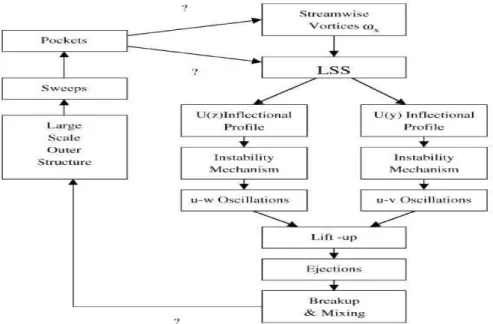
Figure 1.7: Schematic of self-sustaining mechanism with inflectional instabilities. Adopted from (7) (in (77)).

Blackwelder (1998) (7) noted that U (y, z) profile of a streak also has inflec-tions in the z-direction. Figure 1.7 illustrates the self-sustaining relainflec-tionships envisioned by (7). The figure shows instability mechanisms in both U (y) and U (z). A question mark indicates uncertain interactions and obscure mechanisms. On the other hand, the study of Brandt et al. (2003) (14) was motivated by the conjecture that the streak instability, being essentially wake-like in the span-wise direction, could give rise to an absolute instability, as in classical wakes, and then turbulence. Their conclusions do not confirm this conjecture; the streak instability is produced sufficiently high above the wall, in regions where local streamwise velocities are large so that perturbations are “advected away”. Con-cerning the transition to turbulence, it is important to note that the relation of the modal secondary instability to streak breakdown has not been definitely proved (see also the premise of streaks-instability in general, later on).

1.7.2 Minimal flow unit

The minimal flow unit is a concept introduced by Jimenez & Moin(1991)(49). They used the DNS code developed by Kim et al. (1987)(50) for a turbulent channel and reduced the size of the channel width. The idea is to isolate a basic process of wall turbulence. When the spanwise box width is large enough, turbulence can be maintained on only one wall. The flow has only one streak and a streamwise vortex. Calculations confirmed that the cycle is regenerative,

(27)

18 Introduction

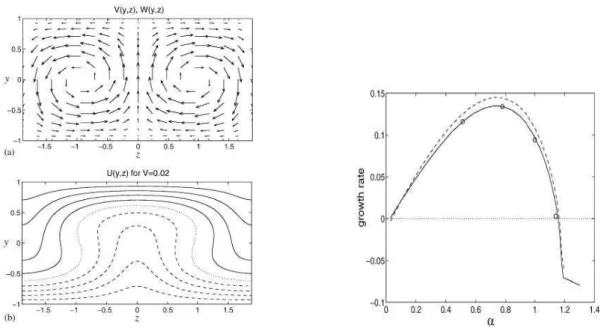
Figure 1.8: Left: (a) Streamwise vortices (0, V (y, z), W (y, z)) in Couette flow. (b) Contour plot of the initial streak profile U (y, z) produced by the vortices. V = 0.02 is the strength parameter. Right: Growth rate vs. α. From Waleffe (1997).

however, it had an unrealistically long time scale, perhaps because of strong viscous effects. Jimenez & Pinelli (1999) (48) continued along this approach. A noteworthy difference was that the channel was wider, wide enough for two or three streak profiles in the spanwise direction and the flow could also contain some large-scale outer structures. By various artificial modifications to the calculations, they tested the viability of the streak instability mechanism and the parent-offspring mechanism. They concluded that a streak instability cycle is possible and entirely exists in the near wall region. This self-sustaining cycle needs no interaction with the outer region. On the other hand, the parent-offspring cycle did not appear viable under these severely viscous conditions. As the authors noted, these conclusions might be modified at higher Reynolds number and/or for larger domains. However, they believed that the streak instability mechanism is the dominant self-sustaining mechanism.

1.7.3 Streaky velocity profiles

We discuss here the “instability” study of the streak profile U (y, z). Waleffe & Kim (1998)(102) and Waleffe(1997) (103) investigated the stability and re-generation of streak profiles in pCf. The streaky velocity profile is produced as follows. Starting with the linear laminar profile, they impose streamwise vortices

(28)

1.7 Instability-based mechanisms 19

structures that extend across the whole channel. After about a quarter of a rev-olution the vortices redistribute the flow to produce the streaky profile U (y, z) as given in figure 1.8 (a, b). Then, the streaky profile is analyzed using linear viscous equations. They impose a perturbation of a form that is sinuous in the x-direction,

v = exp(λt)exp(iαx)Xvn(y) sin(nγz).

Results for the most unstable fundamental sinuous mode are shown in figure 1.8. The maximum growth rate for a spanwise mode with γ = 5/3 is 0.135 for a wavenumber α = 0.74. Within this streak instability, the self-sustaining process proposed by Waleffe (1997) (103) has the following three events:

• 1- Streamwise rolls redistribute the mean flow to form streak profiles. • 2- A sinuous streamwise disturbance leads to an instability of the streak

profiles.

• 3- Nonlinear feedback of the unstable mode injects energy to reform the rolls.

Process (1) is well known. Process (2) is observed in the Gortler flows, but is so sensitive to the used streaky velocity profile and one needs to establish that it occurs in pCf. Process (3) is an essentially new and obscure sequence.

Furthermore, we may wonder if there is a relation between the perturbation spanning all the gap as in Waleffe calculation and the near wall region in turbulent boundary layer. In fact, the Couette flow where these events occur does not have two turbulent wall layers, one on either wall, but a turbulent process within the entire channel. However, in (103), the distance between the walls is 40y+ _{units (} This is roughly equivalent to the “buffer region”, in boundary layer terminology). The entire flow might be considered as a wall region with a moving wall on it. Nevertheless, as with the minimal channel calculations, the main supposition is that the major characteristics of the process are similar to those in a traditional wall layer. In other words, the mechanisms underlying the generation of the streamwise vortices spanning all the gap of pCf would be the same in the near wall region of a traditional turbulent boundary layer. This assumption is certainly correct for some range of Reynolds number and it would be interesting to guess whether this Reynolds number is very large or just moderate.

Schoppa & Hussain (2002)(90) examined the turbulent flow that develops in a channel driven by a pressure gradient. They use a minimal channel of L+

x = 300, L+z = 100. In this channel flow a mean U (y) is constructed so that the upper wall is laminar-like and the lower wall turbulent-like. Their first calculation was a linear stability analysis. It identified a sinuous, linear, inviscid instability that only occurs if the streak-profile strength is sufficient. In this analysis the base-flow streak profile is taken as:

U (y, z) = U (y) + ∆u

(29)

20 Introduction

Figure 1.9: Low-speed streak. (a) Realization from DNS of minimal channel. Isosurface where U = 0.55U0: (b) Typical velocity contours in (y, z) plane. Bold line is same in (a) and (b). (c) Similar contours for profiles used in stability

calculations. Streak strength parameter θ20 = 56 is shown. (d) Mean velocity

profile for half-channel. Adapted from (90).

Here β is chosen to give a streak spacing of 100 and η chosen to give a plateau

in y-vorticity at y+ _{= 10}_{− 30. Instead of using} ∆u

2 to indicate the strength of

the streak profile, a more physical concept was introduced. The streak profile

strength is denoted by θy+, the maximum inclination of a base-flow vortex line

at y+. This occurs on the flank of the streak. Figure 1.9 shows the base-flow

profile and the (y, z) plane velocity contours with θ20 = 56 indicated. Results

of the stability analysis (the growth rate vs. the streamwise wavenumber) show that only streaks with θ20≥ 48 are unstable. Schoppa & Hussain did not believe that linear instability is a dominant mechanism in the self-sustaining process. They used the database of [Kim et al. (1987)(50) and found that the unstable streaks were only a small fraction of the streak population. Thus, the occurrence of a normal mode mechanism was small. In addition, they noted that the time scale for viscous diffusion to destroy the streak profile was short. For example,

a streak profile with intensity θ20 = 56 decayed to θ20 = 50 in t+ = 30. The

third reason was that normal mode growth rates were very small. For example

the most unstable mode for θ20 = 56 grew by a factor of two when diffusion of

the base flow was included.

As described earlier, researchers became aware of non-normality and they started to appreciate that a normal mode stability analysis is only a partial answer. The non-self adjoint nature of the Navier-Stokes equations means that

(30)

1.8 Conclusions of the chapter 21

the unstable normal modes are not the only mechanism of perturbation growth. Perturbations grow algebraically to large levels and then die off exponentially or become an unstable normal mode. The important point is that when the disturbance is at a large level, it is essentially a new flow pattern that can initiate other events. Schoppa & Hussain (2002) (90) chose a perturbation in the form:

w = W sin(αx)yexp(_−ηy)

i.e. not a normal mode (but belongs to the eigen subspace if η is degenerate). They compared the energy of a normal mode and a transient perturbation, de-noted as streak transient growth STG, as a function of time. The transient perturbation grew by a factor of 20 compared to the normal mode’s growth of a factor of two. According to the author’s minimal channel calculations, the perturbation continued to grow to a level where nonlinear equations had to be used. The DNS calculation yielded a regeneration of the streamwise vortex. Here starts the second part of the work of (90). They found that the stretching of the streamwise vorticity ωx by the streak waviness ∂xu, i.e. the term ωx∂xu, caused formation of a streamwise vortex, x-elongated region of ωx. Presumably the cycle was then completed by formation of a new streak profile by this vortex. In this thesis, our findings are compared to the results of (90) (chapter 5).

1.7.4 Conclusions on instabilities

The idea that streamwise vortices are created by the breakdown of the lifted streak due to its inflectional point in the (x, y) plane is legitimate but arguing that, in turbulent pCf, the streamwise vortices result from an inflectional in-stability would be unwarranted. As noted by Schoppa & Hussain (2002) (90) themselves, the occurrence of such instability in turbulent flow has to be proved. Its nature and its origin have to be explained too.

1.8 Conclusions of the chapter

Transition to turbulence in pCf is marked by a competition between patches of turbulent flow scattered amidst laminar flow. Hence, a detailed understanding of this transition to turbulence (globally subcritical) via turbulent spots nucleation and growth, relies on (i) an understanding of microscopic processes such as the self-sustainment of turbulence and (ii) the mechanism by which it propagates into the laminar domain. Unfortunately, elements of answer to these problems are expected perhaps no longer from the detailed study of output of direct nu-merical simulations or experiments, as shown in this chapter, but rather from modeling that might provide heuristic explanations to be further tested in ex-periments either in the laboratory or in the computer. Most rational modeling

(31)

22 Introduction

approaches are developed through truncations of appropriate Galerkin expansions of the primitive equations. Such approach is the kernel of the next chapter.

(32)

Chapter 2 Modeling plane Couette flow

2.1 Introduction

Plane Couette flow which is stable for all R, experiences a discontinuous transi-tion marked by a competitransi-tion between turbulent spots, i.e., patches of turbulent flow scattered amidst laminar flow and separated from it by well defined fronts. A detailed understanding of this transition to turbulence via turbulent spots nu-cleation and growth, relies on an understanding of microscopic processes such as the self-sustainment of turbulence and the mechanism by which it propagates into the laminar domain.

Direct numerical simulations of the Navier–Stokes equations (DNS) have been heavily used to identify elementary processes involved in the sustainment of tur-bulence within the spots. However they produce massive data sets requiring a lot of post-treatment before giving useful hints.

The alternative approach is the development of models at different levels of abstraction depending on the question under scrutinity ((67)). From the obser-vation of near-wall turbulent flow, and its reduction to a so-called minimal flow unit, Waleffe was able to derive a differential model involving the amplitude of a few modes associated to coherent structures ((103)), a Galerkin-like approach that was made more systematic by Eckhardt and co-workers (e.g., (28)). Such models indeed enlighten some of the mechanisms involved in the sustainment of turbulence and the competition between laminar and turbulent states at the fractal border of the basin of attraction of laminar flow according to the abstract phase space viewpoint underlying the concept of temporal chaos. However, their low-dimensional nature does not allow one to approach such problems as spot propagation that require the explicit reference to physical space. When similar questions were posed for convection, i.e. pattern formation, it was found partic-ularly valuable to pass from ordinary differential systems that can only deal with the time behavior, such as the Lorenz model, to partial differential equations (PDE) that also account for space dependence, e.g. the Swift–Hohenberg model

(33)

24 Modeling plane Couette flow

((97)) and its numerous variants, in order to diagnose spatio-temporal chaos. This chapter is concerned with the derivation of a closed set of PDEs appro-priate to the plane Couette flow. This case is particularly interesting since, by contrast with other wall-bounded flows such as the Poiseuille flow or the lami-nar boundary layer (Blasius) flow, it completely lacks linear instability and the absence of downstream advection makes it practical to observe the long term dynamics of spots, a crucial element of the subcritical transition to turbulence.

The space-time dependent models to be developed below are mostly intended to attack the two main problems: how the spots get sustained at moderate R, and how they contaminate the laminar flow.

Contrasting with the regime of developed turbulence taking place at large R, which requires a refined space-time resolution able to account for the cascade toward “small” scales, the transitional regime around Rg involves structures that appear to be “large,” i.e. to occupy the full gap between the plates, and “coher-ent.” In turn, a model in terms of a few well-chosen modes with low wall-normal resolution should be sufficient for describing spots and understanding their dy-namics. The amplitude of these modes will then be taken as functions of the in-plane coordinates. This is the reason why we speak of 2.5-dimensional mod-els. In this terminology, the number 2 stands for the full in-plane dependence (x, z) and the suffix .5 suggestively expresses that the dependence on the third, cross-stream, coordinate y is only partly taken into account through low order

truncation. In the next section §2.2, we present the primitive set of equations

and we derive our no-slip model using the Galerkin method. In _{§2.3, we give a}

glimpse on the derivation of models with stress-free boundary conditions.

2.2 No-slip model

The Navier-Stokes equation and continuity condition for an incompressible flow read:

∂tv + ω.v + 1/2∇v2 = −∇p + ν∇2v, (2.1)

∇_{· v = 0 ,} _(2.2)

where v ≡ (u, v, w), p is the pressure and ν is the kinematic viscosity. Further,

∇2 _{denotes the three-dimensional Laplacian. We have rewritten the nonlinearity}

using the identity v.∇v = 1/2∇v2_{+ ω.v, with ω = ∇}t_v

− ∇v.

In the following we use dimensionless quantities. Lengths are systematically scaled with h, and Up stands for the velocity scale, hence a basic velocity profile

U (y) = Uby for y ∈ [−1, 1] in the no-slip case (Ub = 1). The equations are

(34)

2.2 No-slip model 25

u = U (y) + u′_{, v = v}′_{, w = w}′_{, p = p}′_{, so that (2.1,2.2) accordingly read:} ∂tu′+ (∂yu′ − ∂xv′)v′+ (∂zu′− ∂xw′)w′ + ∂xEloc′ =_−∂xp′− U∂xu′− v′∂yU + R−1∇2u′, (2.3) ∂tv′+ (∂xv′− ∂yu′)u′+ (∂zv′− ∂yw′)w′+ ∂yEloc′ =−∂yp′− U∂xv′+ R−1∇2v′, (2.4) ∂tw′+ (∂xw′− ∂zu′)u′ + (∂yw′− ∂zv′)v′+ ∂zEloc′ =−∂zp′− U∂xw′+ R−1∇2w′. (2.5) 0 = ∂xu′+ ∂yv′+ ∂zw′, (2.6) where E′ loc = 12(u′2+ v′2+ w′2).

The Galerkin method is a special case of a weighted residual method ((32)). It consists here in forcing the separation of in-plane and wall-normal coordinates by expanding the perturbations (u′_{, v}′_{, w}′_{, p}′_{) onto a complete basis of y-dependent} functions satisfying the BCs with amplitudes dependent on (x, z, t). The equa-tions of motion are then projected onto the same functional basis, using the canonical scalar product. The main modeling step is then performed when trun-cating these expansions at a low order and keeping the corresponding number of residuals in order to get a consistent and closed system governing the retained amplitudes. The no-slip boundary conditions for the vertical velocity component are:

v′_{(y =}_{±1) = ∂}

yv′(y =±1) = 0 (2.7)

obtained by combining the continuity equation (2.6) to the conditions

u′(y =±1) = w′_{(y =}_{±1) = 0 .} _(2.8)

To satisfy these conditions, we take a basis made of polynomials in the wall-normal coordinate y, which also forms a family of functions closed for multiplica-tion and differentiamultiplica-tion. We do not use Chebyshev polynomials fully adapted to highly resolved DNS ((6)) because, in spite of their good orthogonality properties, they do not permit a straightforward account of the BCs at the low truncation orders we are interested in. By contrast, we can easily construct individual basis functions all satisfying the BCs arising from the no-slip conditions (2.7,2.8) and develop a strict Galerkin approach ((34)). Projections are performed by taking the canonical scalar product _{h., .i defined by:}

hf, gi = Z +1

−1

f (y)g(y) dy .

It turns out that things are simple only when restricting consistently to the lowest possible order, i.e. keeping only functions associated to U0, W0, U1, V1, and W1, due to the parity properties of the functions involved that automatically guarantee the orthogonality of the different contributions to the velocity field.

(35)

Boundary conditions (2.7) suggest one to take ((34; 66)): v′ _{= V}

1A(1− y2)2, (2.9)

and accordingly (2.8): {u′_{, w}′_{} = {U}

0, W0}B(1 − y2) +{U1, W1}Cy(1 − y2) . (2.10) The pressure is expanded like_{u′_{, w}′_{}, with two corresponding coefficients P}

0 and

P1 that can be interpreted as the Lagrange multipliers introduced to fulfill the

even and odd lowest order projections of (2.6). The normalization constants are

given by: A2 _{= J}−1

0,4 = 315/256, B2 = J0,2−1 = 15/16, and C2 = J2,2−1 = 105/16. Amplitudes introduced in (2.9,2.10) are all functions of x, z, and t. The drift-flow component (U0, W0) has a plane Poiseuille profile, in close correspondence with what happens in the Rayleigh-B´enard case, as noticed first by (93) and subse-quently exploited to derive the generalized Swift–Hohenberg model described in (66).

According to the Galerkin method prescriptions, we insert the assumed expan-sions (2.9,2.10) in the continuity equation (2.6), then we multiply it by B(1_{− y}2₎ and integrate over the gap, which extracts its even part:

∂xU0+ ∂zW0 = 0 .

In the same way, multiplying (2.6) by Cy(1_{− y}2_{), and integrating it extracts the} odd part that reads:

∂xU1+ ∂zW1 = βV1,

with β = √3. Doing the appropriate manipulations for (2.3) and (2.5), we

straightforwardly obtain the even parts as

∂tU0+ NU0 = −∂xP0− a1Ub∂xU1− a2UbV1 + R−1_(∆ 2− γ0) U0, (2.11) ∂tW0 + NW0 = −∂zP0 − a1Ub∂xW1 + R−1(∆2− γ0)W0, (2.12) with γ0 = 5₂, a1 = 1/ √ 7, a2 = 3 √ 3/2√7, Ub = 1 and NU0 = α2β′U1V1− α3V1∂xV1+ α1W0(∂zU0− ∂xW0) + α2W1(∂zU1− ∂xW1) + ∂xEa, NW0 = α2β ′_V 1W1− α3V1∂zV1+ α1U0(∂xW0− ∂zU0) + α2U1(∂xW1− ∂zU1) + ∂zEa, with α1 = 3 √ 15/14, α2 = √ 15/6, and α3 = 5 √ 15/22, β′ _{= 3β/2 and E} a = 1

(36)

2.2 No-slip model 27 and (2.5) read: ∂tU1+ NU1 = − ∂xP1− a1Ub∂xU0 + R−1_(∆ 2− γ1)U1, (2.13) ∂tW1+ NW1 = − ∂zP1− a1Ub∂xW0 + R−1_(∆ 2− γ1) W1, (2.14) with NU1 = −α2β ′′_U 0V1+ α2W1(∂zU0− ∂xW0) + α2W0(∂zU1− ∂xW1) + ∂xEb, NW1 = −α2β ′′_V 1W0 + α2U1(∂xW0− ∂zU0) + α2U0(∂xW1− ∂zU1) + ∂zEb, with γ1 = 21₂, β′′= β/2 and Eb = α2(U0U1+ W0W1). Finally, the projection over V1 gives us: ∂tV1+ NV1 =−βP1+ R−1(∆2− β 2_)V 1, (2.15) with: NV1 = α3(W0∂zV1+ U0∂xV1)− (α2β)(U0U1+ W0W1) + βEb, and α2β = √ 5/2.

To eliminate the pressure P0 and P1 in Eq. (2.11-2.12) and Eq. (2.13-2.15),

we introduce stream functions (Ψ0(x, z, t), Ψ1(x, z, t)) and velocity potential Φ1(x, z, t) that satisfy the two continuity equations:

U0 =−∂zΨ0, W0 = ∂xΨ0, (2.16)

U1 = ∂xΦ1− ∂zΨ1, W1 = ∂zΦ1+ ∂xΨ1 (2.17)

and βV1 = ∆2Φ1. (2.18)

The velocity U1 has two components, U1p = ∂xΦ1 and U1r = −∂zΨ1, where “p”’

(“r”) denotes potential (“rotational”) component (as well as W1). By contrast,

the velocity U0 has only one rotational component (as well as W0).

The equations governing Ψ0 (Ψ1) are obviously obtained by

cross-differentiating and subtracting the equations for the velocity components (2.11-2.12) ((2.13-2.14)) (the rotational part). Taking the divergence of the equations (2.13-2.14) yields an equation for the pressure which is next used with (2.15) to determine the potential part of the velocity field accounted for by the field Φ1. These equations are:

(∂t− R−1(∆2− γ0))∆2Ψ0 = (∂zNU0 − ∂xNW0)

+a1(3₂Ub∂z∆2Φ1− Ub∂x∆2Ψ1) , (2.19)

(∂t− R−1(∆2− γ1))∆2Ψ1 = (∂zNU1 − ∂xNW1)− a1Ub∂x∆2Ψ0, (2.20) (∂t− R−1(∆2− β2))(∆2− β2)∆2Φ1 = β2(∂xNU1 + ∂zNW1)

(37)

The linear term −a1Ub∂x∆2Ψ0 in Eq. 4.6 comes by cross-differentiating the two linear terms _−a1Ub∂xU0 and −a1Ub∂xW0 in Eq. 2.13 and Eq. 2.14. In the same manner, the linear term a1(3₂Ub∂z∆2Φ1 − Ub∂x∆2Ψ1) in Eq. 4.5 comes from −a1Ub∂xU1− a2UbV1 and −a1Ub∂xW1 in Eq. 2.11 and Eq. 2.12.

Note finally that the nonlinear terms can be written by developing the quan-tity Ea and Eb: NU0 = α1(U0∂xU0+ W0∂zU0) + α2(U1∂xU1+ W1∂zU1 + β ′_V 1U1) , (2.22) NW0 = α1(U0∂xW0+ W0∂zW0) + α2(U1∂xW1+ W1∂zW1+ β ′_V 1W1) ,(2.23) NU1 = α2(U0∂xU1+ U1∂xU0+ W0∂zU1+ W1∂zU0− β ′′_V 1U0) , (2.24) NW1 = α2(U0∂xW1+ U1∂xW0+ W0∂zW1+ W1∂zW0− β′′V1W0) , (2.25) NV1 = α3(U0∂xV1 + W0∂zV1) . (2.26)

The benefit of using the first formulation for the nonlinear terms is now clear: The number of FFTs to be performed is roughly divided by two, since only the cross-derivatives of the velocity are computed (∂zU0, ∂xW1, etc...).

On the other hand, the equation governing the mean value of the streamwise velocity component U1, denoted by U1 =R_DU1ds/D is easily obtained by aver-aging Eq. 2.13 over the periodic domain and using the continuity equations and reads:

d

dtU1 = α2(β + β ′′_)U

0V1− γ1R−1U1. (2.27)

For the spanwise velocity component W1, we have:

d

dtW1 = α2(β + β ′′_)W

0V1− γ1R−1W1. (2.28)

The mean value of V1 is governed by:

d

dtV1 =−βP1− R

−1_(∆

2− β2)V1. (2.29)

The mean value of P1 is chosen zero P1 = 0 and hence V1 obviously cancels.

Finally, the mean values of U0 and W0 are governed by the equations:

d dtU0 = α2(β− β ′_)U 1V1− γ0R−1U0, (2.30) d dtW0 = α2(β− β ′_)W 1V1− γ0R−1W0. (2.31)

The average velocity components (U0, U1,...) have to receive a special treat-ment. They are computed in parallel by integrating Eq. 2.27-Eq. 2.31. This is further explained in the next chapter. In the following, we recall the models derived for the stress-free boundary condition and some related results (§2.3.3).

(38)

2.3 Free-slip model 29

2.2.1 Reynolds stress

−U

0

V

1

The evolution equation for the disturbance kinetic energy is the Reynolds-Orr

equation: dE

dt = P − D, where E(t) =

1 2

R

V(u′2 + v′2 + w′2) dV and the two terms on the right-hand side represent the exchange of energy with the base flow

U = Uby i.e. the production P = −

R

V u′v′∂yU dv and energy dissipation D due to viscous effects. The velocity components (u′_{, v}′_{, w}′_{) are the perturbations to} the basic flow U , given by (Eq. 2.9-Eq. 2.10). After integrating over y, we have P =−RDx,zχU0V1ds, where χ is a positive constant.

One reason this equation is interesting is that the occurrence of the two events (U0 negative, V1 positive) or (U0 positive, V1 negative) produce positive Reynolds stress−U0V1 and hence are very significant events in the production of turbulence (in the literature, they are called Q2 and Q4 events, as seen in §1.4.2) .

The linear deformation of the base flow by a vertical velocity is the well known lift-up mechanism (or “effect”) (see e.g.(88)). The generated streamwise velocity by this mechanism is called a streak. In our model, this mechanism is represented by the linear term _−a2UbV1 in the equation (2.11) and U0 represents the streak. It is clear that when the lift-up feeds energy into the system (i.e., V1 generates U0), we have positive Reynolds stress, −U0V1 > 0. The origin of this lift-up are the streamwise vortices, which justifies their dominant role in turbulence production. The central issue addressed in the chapter IV concerns the generation of the streamwise vortices.

2.3 Free-slip model

2.3.1 Derivation

Models for the stress-free boundary condition have been introduced and used in (60) and in (64). We recall here the main steps of their derivation, just in order to compare the structure of the model, obtained by the lowest order trun-cation, to that of the no-slip model, both qualitatively (nature of the terms) and quantitatively (value of coefficients).

Stress-free conditions on the cross-stream velocity (v′_{) read: v}′_{(y =} _{±1) =} ∂yyv′(y =±1) = 0, which directly leads one to take:

v′ ₌X

k≥1

V_2k−1cos((2k_{− 1)βy) + V}2ksin(2kβy) , (2.32)

with β = π/2. For the in-plane components (u′_{, w}′_{), from the continuity equation} (2.6) one obtains ∂yu′(y = ±1) = ∂yw′(y = ±1) = 0, so that the corresponding

Modeling the transition to turbulence in plane Couette flow

HAL Id: pastel-00675068

https://pastel.archives-ouvertes.fr/pastel-00675068

Modeling the transition to turbulence in plane Couette

flow

Maher Lagha

To cite this version:

´

Ecole Polytechnique

Laboratoire d’Hydrodynamique

Thèse présentée pour obtenir le grade de

DOCTEUR DE L’´

ECOLE POLYTECHNIQUE

Spécialité : Mécanique

par

Maher LAGHA

Modeling the transition to turbulence

in plane Couette flow

soutenue le 8 d´ecembre 2006 devant le jury compos´e de :

Foreword

Contents

Chapter 1

Introduction

1.1

Transient lifetimes

1.1.1

Introduction

1.1.2

Numerical and experimental studies

1.2

Turbulent spots

1.2.1

Introduction

1.2.2

Characteristics of turbulent spots

1.3

Spreading mechanisms

1.4

Self-sustainment of wall-turbulence

1.4.1

Definition of coherent structures

1.4.2

Kinetic energy production

1.5

Characteristics of self-sustaining

mechanisms

1.6

Self-replicating mechanisms

1.7

Instability-based mechanisms

1.7.1

Inflectional profiles

1.7.2

Minimal flow unit

1.7.3

Streaky velocity profiles

1.7.4

Conclusions on instabilities

1.8

Conclusions of the chapter

Chapter 2

Modeling plane Couette flow

2.1

Introduction

2.2

No-slip model

2.2.1

Reynolds stress

−U

V

2.3

Free-slip model

2.3.1

Derivation