Control of AFMs in contact mode

Control of AFMs in Contact Mode

by

Khalid E-Rifai

Submitted to the Department of Mechanical Engineering

in partial fulfillment of the requirements for the degree of

Master of Science in Mechanical Engineering

at the

MASSACHUSETTS INSTITUTE OF TECHNOLOGY

Dvne- LUC)3

May 2003

@ Khalid El-Rifai, MMIII. All rights reserved.

The author hereby grants to MIT permission to reproduce and

distribute publicly paper and electronic copies of this thesis document

in whole or in part.

A uthor ...

Department of Mechanical Engineering

May 23, 2003

Certified by ...

...

Kamal Youcef-Toumi

Professor

Thesis Supervisor

Accepted by...

Ain Sonin

Chairman, Department Committee on Graduate Students

MASSACHUSETTS INSTITUTE

OF TECHNOLOGY

Control of AFMs in Contact Mode

by

Khalid El-Rifai

Submitted to the Department of Mechanical Engineering on May 23, 2003, in partial fulfillment of the

requirements for the degree of

Master of Science in Mechanical Engineering

Abstract

The Atomic Force Microscope (AFM) is a high precision surface characterization tool commonly used in Nano-technology, Bio-technology, semiconductors, MEMS, and life sciences' applications. As most versatile systems, AFM offers little guarantees on achieving repeatable satisfactory operation. This is the case as AFMs are not used to perform a single predictable task. AFM systems are feedback regulators, which rely on photodiode detector (PSD) sensing and piezoelectric actuation. The change in probe-surface contact is a disturbance created by scanning across a surface. This disturbance is to be rejected to maintain probe-surface contact and thus allow proper surface characterization. AFM feedback systems are not only required to maintain a nominal PSD output but also guarantee that the control signal used is representative of the rejected disturbance. This is due to the fact that the image of the scanned surface is created from this control voltage. These characteristics impose severe limitations on the system's operation bandwidth, repeatability, and precision. In this effort, the key characteristics and limitations of AFM operation are analyzed. Challenges due to surface variations, plant dynamics, and contact nonlinearity are presented. The closed loop response of AFM systems in single actuator as well as in dual actuator configurations is evaluated. The emphasis is on the underlying structure corresponding to each configuration and not on a particular system tuning. In this regard, the bounds on achievable performance in each configuration are contrasted for operation within the system's overall objectives.

Thesis Supervisor: Kamal Youcef-Toumi Title: Professor

Acknowledgments

I would like to start with my advisor Kamal, the director of the Mechatronics Research Laboratory (MRL). My experience with Kamal has been great on both the intellectual and personal level. His advice has significantly impacted my views about the system dynamics and control area on both practical and theoretical fronts. I would like to specially thank him for his dedication, patience, and support during the preperation of this document.

In here, I must include my brother Osamah, who has been my main source of inspiration all through my academic career. Osamah, a reasearch scientist in MRL, has been working with Kamal for the last few years including his Ph.D. work. His expertise in AFM systems as well as his insight into dynamics and control have been very valuable assets to this effort.

Finally, I would like to extend my thanks to all the great people I recievd my dynamics and control education from both at Purude and MIT. Your comments and advice are intangible references to this work.

Contents

1 Introduction 11

1.1 Problem Formulation . . . . 11

1.2 Literature Survey . . . . 12

1.3 Thesis Scope and Organization . . . . 14

2 Modeling of AFM Dynamics 15 2.1 AFM Operation ... 15

2.2 Dynamical M odel ... . 17

2.2.1 Model Characteristics ... ... 17

2.2.2 System Equations ... ... 19

2.3 AFM Feedback Configurations ... 22

2.3.1 Single Actuator Configurations . . . . 23

2.3.2 Dual Actuator Configuration . . . . 25

2.4 Sum m ary . . . . 26

3 AFM Objectives and Limitations 29 3.1 System Objectives . . . . 29

3.1.1 Single Actuation Objectives . . . . 31

3.1.2 Dual Actuation Objectives . . . . 34

3.2 Fundamental Limitations . . . . 36

3.2.1 Surface variations . . . . 36

3.2.2 Contact Nonlinearity . . . . 37

3.3.1 Single Actuator Systems . . . . 41

3.3.2 Dual Actuator Systems . . . . 46

3.4 Sum m ary . . . . 47

4 AFM Controller Design 49 4.1 AFM Control Problem . . . . 49

4.2 Piezotube Actuator System . . . . 51

4.2.1 PID Controllers . . . . 53

4.2.2 Higher Order Controllers . . . . 55

4.3 Piezocantilever Actuator System . . . . 57

4.3.1 PID Controllers . . . . 57

4.3.2 Higher Order Controllers . . . . 59

4.4 Dual Actuator System . . . . 60

4.4.1 PID Controllers . . . . 61

4.4.2 Higher Order Controllers . . . . 62

4.5 Summary . . . . 64

5 Conclusions and Recommendations 67 A Controller Design 75 A .1 PID control . . . . 75

A.1.1 Piezotube Actuator System . . . . 75

A.1.2 Piezocantilever Actuator System . . . . 75

A.1.3 Dual Actuator System . . . . 76

A.2 H, Synthesis . . . . 76

A.2.1 Single Actuation . . . . 76

A.2.2 Dual Actuation . . . . 78

B MATLAB Codes for H,, Design 81 B.1 Single Actuator Code . . . . 81

List of Figures

2-1 Principle of AFM operation. . . . . 16

2-2 Sample AFM 3-D image. . . . . 17

2-3 Schematic of AFM dynamical model. . . . . 18

2-4 Schematic of a 1-DOF piezoelectric element strain. . . . . 19

2-5 Block diagram of AFM single actuator configurations. . . . . 24

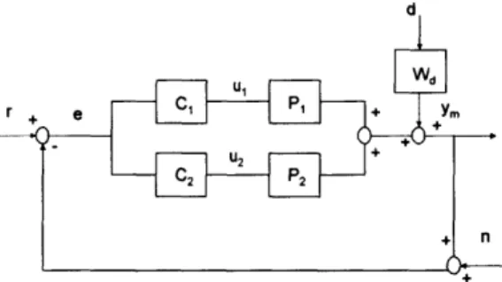
2-6 Block diagram of AFM dual actuator configuration. . . . . 26

3-1 Sample experimental AFM signals: (a) control (height) signal, (b) error (deflection) signal. . . . . 30

3-2 Block diagram of AFM single actuator configurations. . . . . 31

3-3 Single actuator systems objectives in the frequency domain: (a) sensi-tivity, (b) control sensitivity. . . . . 32

3-4 Block diagram of AFM dual actuator configuration. . . . . 34

3-5 Dual actuator systems objectives in the frequency domain: (a) sensi-tivity, (b) control sensitivity. . . . . 35

3-6 Effect of scan speed on the topography induced disturbance: (a) low scan speed experiment, (b) high scan speed experiment. . . . . 38

3-7 Sample representation as a stiffness element. . . . . 39

3-8 Experimental demonstration of probe-sample loss of contact instabil-ity: (a) control (height) signal, (b) error (deflection) signal. . . . . 40

3-9 Experimental demonstration of image oscillations due to piezotube ac-tuator dynam ics. . . . . 41

4-1 Bode diagrams for piezotube actuation with I control: (a) output sen-sitivity, (b) control sensitivity. . . . . 53

4-2 Step disturbance response for piezotube actuation with I control: (a) error signal, (b) control signal. . . . . 54 4-3 Bode diagrams for piezotube actuation with high order controller: (a)

sensitivity, (b) control sensitivity. . . . . 56

4-4 Step disturbance response for piezotube actuation with high order con-troller: (a) error signal, (b) control signal. . . . . 56

4-5 Bode diagrams for piezocantilever actuation with PI controller: (a) sensitivity, (b) control sensitivity . . . . 58

4-6 Step disturbance response for piezocantilever actuation with PI con-troller: (a) error signal, (b) control signal . . . . 58

4-7 Bode diagrams for piezocantilever actuation with high order controller: (a) sensitivity, (b) control sensitivity. . . . . 60

4-8 Step disturbance response for piezocantilever actuation with high order controller: (a) error signal, (b) control signal. . . . . 60

4-9 Bode diagrams for dual actuation with a PI controller for the piezo-cantilever and I controller for piezotube: (a) sensitivity, (b) control sensitivity. . . . . 62

4-10 Step disturbance response for dual actuation with a PI controller for the piezocantilever and I controller for piezotube: (a) error signal, (b) control signals. . . . . 62

4-11 Bode diagrams for dual actuation with a high order controller: (a) sensitivity, (b) control sensitivity. . . . . 64 4-12 Step disturbance response for dual actuation with high order controller:

(a) error signal, (b) control signals. . . . . 64

A-1 H, synthesis set-up for single actuation. . . . . 77

Chapter 1

Introduction

In today's age of nano-technology, nano-scale data have become performance indices in many industries. Furthermore, the detection of chemical and biological phenomena at the atomic-scale has become a basis for many scientific breakthroughs. The Atomic Force Microscope (AFM) has been continuously attracting both industrial and aca-demic organizations as a versatile nano-scale testing instrument. This is attributed to its ability to detect numerous geometric and material properties at strikingly high resolution. AFM has been favored due to its compatibility with many samples and ambient conditions. The use of AFM as a characterization tool is done with no restric-tions on the sample's electrical conductivity or optical permittivity. In addition, AFM has been successfully operated in room conditions, vacuum, and fluid environments.

1.1

Problem Formulation

AFM has become a very popular tool in research and industries of Nano-technology, Bio-technology, semiconductors, MEMS, and life sciences. In terms of usage, AFMs have been used in surface characterization for metrology purposes. This is used to evaluate final geometric tolerances of a product as well as monitor intermediate fabrication products. The AFM has been also used in detecting contrast in frictional, elastic, viscoelastic, magnetic, and electric properties. This has allowed it to become an inspection tool for micro-fabrication processes in many industries. Furthermore,

the underlying principle by which AFM operates has been used to capture many important atomic-scale phenomena using chemically or biologically treated tips. Last but not least, AFM has become a popular tool in micro- and nano- fabrication, most notably in lithography.

AFM is a feedback regulator system with a piezoelectric actuator and a position sensitive photodiode (PSD) sensor. A unique feature here is that the control signal is used to create the scanned sample's image. This introduces restrictions on the system's behavior, which are rarely of concern in most feedback systems. As AFMs are not used to perform a single predictable task, they offer little guarantees on achieving repeatable satisfactory operation. This is further aggravated by the coupling between

user-defined scan and control parameters.

In recent years, many developments have been made to automate and improve the AFM's operation, especially for industrial applications. The list includes the use of optical pattern recognition or additional position sensors to repeatably land on the same scanned location. Automated motion stages have been included to perform a series of imaging routines. Programmable manipulators have been used to automatically load/change samples and probes. Nevertheless, the main operation of the system, the imaging process, remains operated in an ad-hoc trial and error fashion. It is desired to achieve repeatable high precision and bandwidth operation for the full AFM actuation range.

1.2

Literature Survey

The efforts towards enhancing and understanding AFM systems' behavior can be separated into two main directions: a modeling and control approach and a design and fabrication approach.

Recent modeling and control work on AFM systems has lead to a much better understanding of the system's behavior. Several key dynamical characteristics of the AFM have been modelled and identified in [1, 2, 3, 4]. Other studies include design and simulation of an output feedback linearization control law using a nonlinear model

for the AFM [15]. However, the model used only includes the cantilever dynamics. In here, a main limiting factor, the piezotube actuator dynamics, has been neglected. In addition, an H, controller synthesis has been used in [9] to design a controller for an experimentally identified model. As reported by the authors, their control implementation lead to five times faster scanning speed than obtained using a tuned PID controller. However, this was at the expense of the control signal containing significant oscillations even at steady-state. As a result, the scanned sample's image, i.e., the control signal, was not recordable.

Meanwhile, a parallel group of work has been focusing on the actuator design aspect. The AFM has been primarily actuated by piezoelectric tube actuators. Other actuation schemes as well as different piezotube designs have been considered. As far as piezotube scanners' design, a limiting trade-off between vertical travel range and bandwidth has been arrived at. More recently, along with developments in MEMS fabrication, a piezoelectric film has been patterned onto cantilevers allowing for an alternate actuation scheme [10, 13, 14, 11]. Various designs have been attempted and validated until this actuator, a piezoelectric cantilever, became commercially available. Experiments have been performed on a chosen sample to demonstrate an improvement in bandwidth with this actuator [13, 10, 11, 14]. Though such design has been found to allow for much faster scanning speeds, while maintaining imaging precision, it further sacrifices imaging range. In addition, it has been desired to use dual actuation in order to overcome the trade-off between actuator bandwidth and range. It has been demonstrated, for a selected sample, that the piezoelectric cantilever can be combined with a coarse actuator to achieve accurate imaging. In this context, the coarse actuator was a thermal actuator in (16] and a piezotube in

[17]. Yet, it is not understood whether a performance improvement would be achieved

with dual actuation. The use of the piezocantilever along with the piezotube needs to improve over the performance achieved with a sole piezotube actuator. This has limited the use 6f the piezocantilever actuator to sole actuation in some applications where only small vertical imaging range is needed. In fact, since the system's behavior depends on the scanned surface, very little knowledge is available on the expected

performance for different actuation configurations. As a result, most AFMs remain operated in the conventional setting with a piezotube actuator despite its limitations.

1.3

Thesis Scope and Organization

A comprehensive model of the AFM dynamics spanning THE MAIN actuation

config-urations, is developed. The fundamental limitations on achieving the system's overall objectives are presented. Challenges due to surface variations, plant dynamics, and contact nonlinearity are analyzed. Furthermore, the system's performance in single actuation configurations as well as in dual actuation is evaluated. In this regard, different controller design algorithms are used in order to demonstrate the feedback system's performance bounds in each configuration.

The remaining parts of this document are organized as follows. Chapter 2 presents a dynamical model of AFM operation, which includes single and dual actuation con-figurations. Next, the objectives and limitations of contact mode AFM feedback systems are presented in Chapter 3. System configurations of single actuation with a piezotube and a piezocantilever as well as dual actuation are analyzed and contrasted. In Chapter 4, a controller design analysis is performed, based on experimentally iden-tified models. This analysis is used to evaluate the limiting system behavior for each configuration. Concluding remarks and recommendations are given in Chapter 5.

Chapter 2

Modeling of AFM Dynamics

In this chapter, the basic principle of contact mode AFM operation is reviewed. A model of the overall AFM dynamics is presented. Then, system configurations of single actuation with either a piezoelectric tube or a piezoelectric cantilever as well as dual actuation are presented.

2.1

AFM Operation

The basic principle of the AFM operation is based on using a micro-cantilever with a sharp object at its tip to probe a scanned surface. The cantilever is mounted on a piezoelectric tube scanner, which can translate both laterally and vertically, see Figure 2-1. As the probe touches a feature on a surface, it generates a force causing the cantilever to deflect. Therefore, light from a laser source reflects off the cantilever's

tip and the corresponding change in cantilever deflection is recorded via a position sensitive split photodetector (PSD). This sensor measurement is then compared to a chosen setpoint detector voltage, reflecting a nominal setpoint cantilever deflection. The difference between the current sensor output and nominal output is then sent to a controller. The controller causes the scanner to extend or retract via an input voltage in order to maintain the nominal detector setpoint. The operation continues as the AFM is ordered to raster scan across a sample with a prescribed scan size. This leads to continuous extension and retraction of the scanner following vertical

surface variations. The recorded surface height is the control signal in volts scaled

by the calibrated sensitivity of the piezoelectric actuator in nanometers/volts. The 3-D surface image is generated from the height data and the user-defined lateral scan

area and sampling resolution.

Piezotube X Detector (PSD) Laser Cantilever Z Probe Sample

Figure 2-1: Principle of AFM operation.

Furthermore, AFM in contact mode has been used to collect surface frictional and tribological properties. This is made possible by the four-quadrant PSD, which records the relative intensity of the reflected laser beam in both the lateral and vertical directions. In this regard, the vertical and lateral deflections of the laser beam account for the deflection of the cantilever due to bending and torsion, respectively. Here, variations in the lateral cantilever deflection represent frictional surface variations.

Whereas, tapping mode AFM is similarly operated but rather with intermittent contact with the sample. This is achieved by driving the cantilever through a har-monic excitation near its resonant frequency. The task of the feedback controller is to maintain a constant root-mean-square (RMS) cantilever deflection. In this re-gard, tapping mode is preferred over contact mode for soft biological surfaces since lateral motion of the probing tip is performed in air. This eliminates scraping or frictional affects induced by maintaining continuous contact. Nevertheless, contact

mode AFM surpasses tapping mode in terms of achievable resolution and allowable scanning speeds.

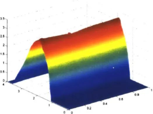
Figure 3-2 is a 3-D image of a sample from a thin-film deposition fabrication process, with a scanned spot of 4pm x 1pm. Note that the flat regions in the map are due to reaching the piezotube 's vertical travel limit, which is about 3pm. Here, lateral and vertical variations in the product's edge are characterized by RMS values of 12 nm and 48 nm, respectively.

Figure 2-2: Sample AFM 3-D image.

It is important to realize that AFM's compatibility with various ambient condi-tions and sample properties comes at a cost. The ability to acquire an image of a sample depends on the cantilever-probe assembly used as well as the chosen scan and control parameters.

2.2

Dynamical Model

2.2.1

Model Characteristics

The system's dynamics of interest are characterized by the three degrees-of-freedom in Figure 2-3. Here, z, is the extension of the piezotube, Op is the piezotube bending, and 0, is the cantilever bending relative to the tube base.

zP

Figure 2-3: Schematic of AFM dynamical model.

Here, the piezoelectric tube extends or retracts, zp, in response to an input voltage. Though it is desired that the tube only extends and retracts to a given voltage, this ideal behavior is not achieved in practice. A small piezotube bending in response to this input voltage is usually observed due to inevitable tube eccentricity. Therefore, it is necessary to include the bending of the tube Op as it affects the cantilever bending dynamics. Coupling between extension and bending dynamics of piezotube scanners used in AFMs was 1" reported in [2]. The 3rd included degree-of-freedom is the cantilever bending, 0c, which is the variable to be controlled in the system. These are the only degrees-of-freedom of interest in terms of the vertical dynamics.

Note that the model is only concerned with the vertical dynamics. In AFMs, the control action is concerned with the vertical and not the lateral dynamics of the scan-ner. The lateral motion, i.e., the scanning, is prescribed by the choice of the scanned spot size and the sampling resolution. Then, at each (x, y) point a voltage is given to the piezoelectric actuator to extend or retract in the vertical direction. Therefore, no additional degrees-of-freedom need to be included in order to represent the system's operation.

The displacement z of a piezoelectric element in response to an input voltage u is represented in Figure 2-4. This characterizes the dynamics of a single piezoelectric actuator mode with one actuator end fixed. Here, M, k, and c are the effective inertia, stiffness, and damping of this flexible mode.

z

k

F

M U

Figure 2-4: Schematic of a 1-DOF piezoelectric element strain.

It is important to note that the absolute position and velocity of the probe is not only a function of Oc but also depends on O, and z,. This is the case since the cantilever's bending 0, is defined relative to the tube base.

2.2.2

System Equations

The following section presents the equations of motion governing the system's dynam-ics of interest. In this regard, the 1 mode of each of the discussed three degrees-of-freedom will be considered. This requires an appropriate system bandwidth in order to attenuate the effect of higher frequency unmodeled modes. This is inevitably the case as this feedback system is to be operated within a finite bandwidth. A detailed analysis of the system operation bandwidth and unmodeled dynamics for each actu-ation configuractu-ation is performed in the next chapter. Therefore, a 3-DOF lumped parameter model of the system can be represented by Equations (2.1-2.4). Here, the

1" three equations describe the dynamics of each DOF and the fourth equation is the

measurement.

, + 2(opwop6 p + W26 = aopul (2.1) ip + 2(2p(2zpi + , z = apu(2.2)

Oe + 2(cw6c~ + (A2c = a1,6 + b1O, + a2i,

+

Ym = Oc + Op (2.4)

The 1" two differential equations describe the dynamics of the two piezotube

flex-ible modes of interest. The voltage given to the piezotube generates tube strain in the extension and bending modes. Each one of these piezotube modes can be represented

by the schematic in Figure 2-4, where the input voltage u = u1. This is evident as

the tube top end is fixed as shown in Figure 2-3. Here, the only inputs acting on the tube are the input voltage ui as well as reaction forces from the cantilever. The latter are neglected since the forces created by the cantilever are at most of the order of 100pN. This is due to the fact that the maximal micro-cantilever stiffness is of the order of 10's N/m and its maximum possible deflection is of the order of a few pUm. This reaction from the cantilever is compared to the load capacity of a typical AFM piezotube, which is about a few Newtons.

The 3" equation describes the cantilever bending dynamics. Note the inclusion

of acceleration terms from both piezotube modes in the right hand side of Equation

(2.3). This is attributed to the fact that the cantilever bending 0, is a relative and not

an absolute coordinate. Where velocity terms from the piezotube modes are intro-duced to represent the dissipation in the probe-sample contact. The dampening effect imposed on the cantilever's dynamics due to contact depends on the relative velocity between the probe and the sample. For a stationary sample, this relative velocity is that of the probe absolute velocity, which depends on the piezotube extension i, and bending dp.

due to contact with the sample fcontact. This probe-sample force is a function of the relative position between the probe and the contacted surface. Hence, it is a function of the absolute position of the probe as well as the sample height. Therefore, piezotube bending O, and extension z, terms need to be included to represent the absolute probe position. In this regard, changes in the contact force, including any nonlinear terms, will be represented as an external disturbance d. This disturbance accounts for changing the cantilever deflection during scanning. The following approximation of the force fcontact will thus be used, where ci and c2 are motion coupling coefficients

between the cantilever and piezotube:

fconitct C1Op + C2Zp + d (2.5)

Furthermore, the input voltage u2 is also included in Equation (2.3) if the

can-tilever is a piezoelectric self-actuated cancan-tilever, where aoc is a gain. Here, a thin piezoelectric film is patterned along most or all of the length of a silicon cantilever. This suggests that the dynamics of the piezoelectric cantilever in response to input voltage u2 follows the representation in Figure 2-4. Note that the structural dynamics

of the cantilever, of resonance wc, is then associated with the combined piezoelectric and silicon layers.

Finally, Equation (2.4) represents the fact that the photodiode sensor collects the absolute angular deviation of a laser beam reflected off the cantilever. Therefore, the measurement is the sum of the piezotube bending and cantilever bending relative to the tube base. Note that no dynamics is introduced from the sensor as it is a non-contact sensor. Here, the bandwidth of the sensor is of the order of 1014 Hz, based

on the typical wavelength and speed of light. It is noteworthy that low pass filters are usually used to filter out high frequency measurement noise. Here, the bandwidth of such filters varies depending on the sensor electronics used in the system.

In this effort, a linear-time-invariant model is used to capture the system's essential dynamics. The most notable nonlinearity in the system's dynamics is associated with the probe-surface contact. The contact force fcontact is a nonlinear force of

the probe-sample separation, which depends on the ambient as well as contacting objects' geometric and material properties. Here, retaining only the linear terms, Equation (2.5), leads to lumping the effect of surface variations including nonlinear terms of fcontct in the external input d. In addition, the voltage-strain relation of a piezoelectric element is also known to exhibit some nonlinearity. In here, the effect of the aforementioned nonlinearities accounts for uncertainties in the this linear model

driven by an external disturbance d.

It is noteworthy that this model is in agreement with that derived in [1] for piezotube actuated systems. Experimental frequency response results of the piezotube dynamics as well as the piezocantilever have been reported in [1, 2, 3, 4, 14, 12]. Typical values of piezotube bending, piezotube extension, and cantilever bending 11t resonances are of the order of a few hundred Hz, a few kHz, and tens of kHz, respectively.

Commercially used micro-cantilevers are of a 11t bending mode resonance in the

10 - 100kHz range, as suggested by typical vendor specifications [36]. Note that the cantilever properties in the conventional setting, where a piezotube is the only actuator, can vary significantly depending on imaging requirements. Whereas, typical commercial piezoelectric cantilevers are of a 1" resonance at 40 - 60kHz [35].

On the other hand, extension piezotube actuators used in AFM are of a typical vertical travel in the 5 - 6pm range. Commercial piezotube actuators of such range are of a 1" bending and extension resonance in the few hundred Hz and few kHz ranges, respectively [34].

2.3

AFM Feedback Configurations

In this section the dynamics of AFM operation is represented in the standard linear-time-invariant (LTI) feedback set-up. It is important to realize that AFMs are feed-back systems, as equations (2.1-2.4) follow the standard feedfeed-back control form. The following relation between the detector output y., input voltages ui and u2, and the

Ym = P1u1 + P2u2 + Wd (

Here, the variables yin, u1, U2, and d are in the Laplace domain. The transfer

functions Pi(s), P2(s), and Wd(s) are defined as follows:

Ym (azis2 + bzis + cz1)(az2s2 + bz2s + cz2)

Ui

P

+

M

In the transfer function P(s) the three pairs of complex poles are at the three natural modes of the 3-DOF system. The 1" pair of complex zeros, azis2

+ bzis + czi,

is an anti-resonance associated with the coupling between the piezotube bending mode and the cantilever mode. Similarly, the second pair of zeros is associated with coupling between the piezotube extension and cantilever bending. These zeros seen in P(s) are due to the fact that the cantilever dynamics is not excited by the input voltage ui directly. In fact, the cantilever dynamics are driven by piezotube bending and extension terms, Equation (2.3), which are in turn excited by the voltage u1.

In here, the anti-resonances are within the frequency range of each piezotube mode they are associated with. On the other hand, Wd(s) and P2(s) only contain a pair of

complex poles, the cantilever bending mode, as should be predicted from the system equations. In terms of actuation, the system can be operated in a single or dual actuator configuration.

2.3.1

Single Actuator Configurations

In single actuator systems, the block diagram representing the system is given by Figure 3-2. In this case, a single actuator is used to maintain the output of the detector, ym, at the nominal setpoint voltage, r. Here, the error e is the difference between the current detector output and the nominal setpoint output. Maintaining a small error is used to indicate a maintained constant cantilever deflection. In Figure

2-5, P is the plant transfer function and C is the controller transfer function. The sole

actuator is either a piezoelectric tube or a piezoelectric cantilever. In this regard, the control signal is either u1 or u2 for piezotube or piezocantilever actuation, respectively.

As shown in Figure 3-2, variations in the contacted surface d are represented as an output disturbance with a pre-filter Wd. This representation follows directly from Equation (2.6). In the block diagram, n represents measurement noise for the PSD sensor. This is dominated by shot noise for the PSD as well as noise due to sensor electronics [5, 6, 7].

d

Wd

e C P +

+ n

Figure 2-5: Block diagram of AFM single actuator configurations.

Next, both single actuator configurations with either a piezotube actuator or a piezocantilever actuator are discussed.

Piezotube Actuator Configuration

In this situation, the system is operated in the conventional AFM setting with a piezotube actuator. Here, the cantilever is no longer self-actuated. Therefore, in Equation (2.3), u2 = 0, with the rest of the model unchanged. The block diagram

of this system is associated with a plant, P = P1(s), between the unique output

ym and the control input u = u1 acting on the piezotube. The plant is a 6th order

for detecting topography variations of up to 3 - 5[Lm depending on the piezotube range. The image of the contacted surface is created from the control voltage ui and the calibrated sensitivity of the piezotube actuator in nm/volts.

Piezocantilever Actuator Configuration

Here, the cantilever is self-actuated via an input voltage u2. This is achieved by

using a cantilever with a patterned piezoelectric layer. It is important to note that in this situation the piezotube is not replaced by a piezocantilever but rather no longer actuated by a given voltage to respond in the vertical direction. In fact, the piezotube is still used for lateral scanning. Equations (2.1-2.4) simplify with 9, = ,, =9,, = i, = i, = z, ~ 0 by noting that no control voltage is applied to the

piezotube (ui = 0) and recalling that forces from the cantilever are of negligible effect

on the piezotube strain. Hence, the only degree-of-freedom of interest is the cantilever bending, 0,. In Figure 2-5, the control signal is u = u2 and thus P = P2(s), which

is a 2nd order with no zeros transfer function. Recall that the structural dynamics

of the cantilever, of resonance we, are associated with the combined piezoelectric and silicon layers. This type of actuation may only be used for characterization of surfaces of fine variations in height, which is typically limited to around 500 nm. This is a typical bound based on this actuator travel range. Studies on the fabrication, design, and calibration of such actuators may be found in [10, 11, 13, 14]. In this configuration, the image of the scanned sample is created from the control voltage U2

and the calibrated sensitivity of the piezocantilever actuator in nm/volts.

2.3.2

Dual Actuator Configuration

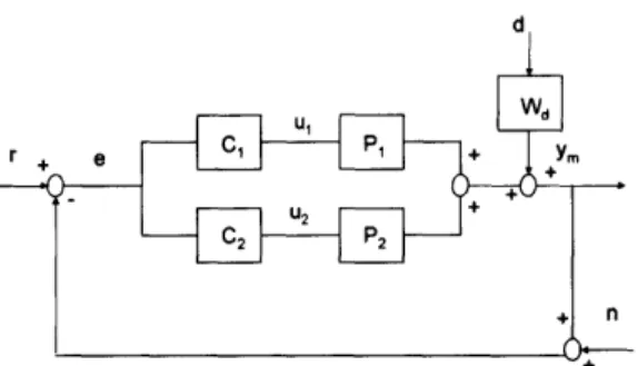
The block diagram representing the dual actuator AFM system is given by Figure

2-6. In this scenario, the piezotube and a piezocantilever are supplied with input

voltages ui and u2, respectively. Where the plants P1(s) and P2(s) are as given in

Equations (2.7-2.8). The control action associated with each plant transfer function is represented by the controller transfer functions Ci(s) and C2(s). Here, the reference

setpoint r, disturbance d, and measurement noise n are as defined earlier. u, Wd r+ C, P1 + ym U2 C2 P2 + n

Figure 2-6: Block diagram of AFM dual actuator configuration.

In this configuration, the combined action of both actuators is used to maintain probe contact with the scanned surface. The detector error e is to be maintained small with the detector output ym following its reference setpoint value r. The piezocan-tilever, a fine actuator, would only be responsible for maintaining contact in response to vertical surface variations within its limited range. Here, the addition of the piezo-cantilever actuator is proposed to improve over the performance achieved with the sole piezotube actuator. Whereas, the piezotube is actuated to allow for detecting topography variations beyond the piezocantilever's range. The recorded surface im-age is thus created from both input voltim-ages and actuator sensitivities in nm/volts.

2.4

Summary

In this chapter, an overall model of the AFM dynamics has been developed. Key system characteristics and modeling assumptions have been discussed. The block

the AFM may be operated in a single or dual actuator configuration. In single actuation, either a piezotube actuator or a piezocantilever actuator is used. In dual actuation, both actuators are used to control the same single output. In addition, the plant characteristics of each configuration have been identified. Here, the variation in the scanned surface is viewed as a disturbance acting at the output. The control action is used to maintain a constant detector output such that probe-surface contact is sustained.

Chapter 3

AFM Objectives and Limitations

The following chapter presents the objectives and limitations of AFM feedback sys-tems. The objectives associated with single and dual actuation configurations are presented. The main fundamental limitations on achieving system objectives due to surface variations and contact nonlinearity are discussed. Feedback structural limi-tations are analyzed and contrasted for the system configurations.

3.1

System Objectives

The task of AFM regulator systems is to reject the effect of variations in the scanned surface on maintaining probe-surface contact. This is verified by maintaining a con-stant setpoint detector output. When a small error between a nominal setpoint and the detector output is maintained the probe is in good contact with the surface. This is performed as the probe is scanned across a sample's cross section. The process continues for a number of cross sections within the prescribed scanned area. As a result, the height of the contacted surface at each point in the scanned area may be obtained. The height of the contacted surface at each scanned point is given by the product of the control voltage sent to the actuator at this point and the calibrated sensitivity of the actuator in nm/volts. This is the case since this product reflects the change in vertical displacement of the actuator used to maintain this contact.

H gh . ... eflection 23.15 m/div

24.9 rndiv24.99 ms/div

(a) (b)

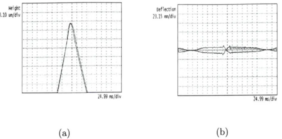
Figure 3-1: Sample experimental AFM signals: (a) control (height) signal, (b) error (deflection) signal.

Figure 3-1 shows the two signals of interest recorded during a selected AFM scan. The scan is made for a triangular silicon grating with an included angle of about

70'. The plot, Figure 3-1(a), shows the sample's height along a scanned cross section,

i.e., the control signal scaled by the actuator's voltage-displacement sensitivity. In addition, the deflection (error) signal is given in Figure 3-1(b). This signal is the difference between the detector's output and the setpoint output to be followed. This detector output is representative of the cantilever deflection. Note that the plot shows two error signals that are mirror images with respect to the horizontal axis. These correspond to the error in lateral scanning in the two possible directions, commonly referred to as trace and retrace. It is important to note that for an inappropriate choice of scan and control parameters, the maximum error shown is about 10 nm as apposed to the theoretically achievable sub-nanometer resolution. This highlights that this theoretical resolution is achieved subject to an appropriate choice of scan and control parameters.

The response of the control (image) and error (deflection) signals to the scanned surface variations, i.e., output disturbance, is governed by the control sensitivity

control sensitivity and output sensitivity functions are defined as follows:

U e

SU = -d so= -d (3.1)

Here, u is a control signal, e is the control error, and d is an output disturbance. More formally, the objectives of AFM feedback systems can be represented through the desired shapes of the output sensitivity and control sensitivity functions in the frequency domain. In this regard, a distinction takes place between single an dual actuation configurations.

3.1.1

Single Actuation Objectives

Recall that single actuator systems are represented by the block diagram given in Figure 3-2.

d

r +

e

Y

+ n

Figure 3-2: Block diagram of AFM single actuator configurations.

Here, a single actuator is used to maintain the output of the detector, y., at the nominal setpoint, r. The difference between the current detector output and the nominal output r is the error e to be maintained small. The sole actuator is either a piezoelectric tube or a piezoelectric cantilever. In this regard, the control signal is either u1 or u2 for piezotube or piezocantilever actuation, respectively. Variations in

pre-filter Wd. Recall that this pre-filter contains the cantilever's dynamics since this disturbance is a force acting on the cantilever. The difference between both actuators

is that the piezocantilever may only respond to topography induced disturbances within its limited range relative to that of the piezotube. As a result, variations in surface height beyond an actuator's travel range are not detected.

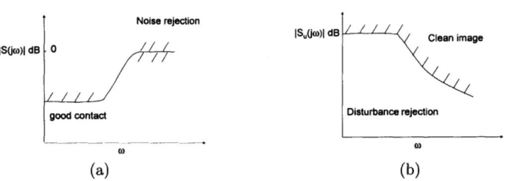
Figure 3-3 describes the desired shapes for the control sensitivity and sensitivity functions in single actuator AFM systems. The sensitivity function, S0, is desired

to be of a small gain at low frequencies up to a maximal possible bandwidth, as in most feedback systems. This suggests that the error e is insensitive to variations in the contact disturbance d within this range of frequencies, see Equation (3.1). As a result, a small error is maintained between the nominal setpoint r and the current output ym suggesting good contact during scanning.

Noise rejection

|SS(o) dB Clean image IS(j0)I dB -0

good contact Disturbance rejection

000

(a) (b)

Figure 3-3: Single actuator systems objectives in the frequency domain: (a) sensitiv-ity, (b) control sensitivity.

The objectives associated with the control sensitivity function are given in

3-3(b). The control sensitivity, S,, represents the response of the control signal to

the topography induced disturbance. It is desired that the frequency response of this transfer function be flat up to a maximal possible frequency. This leads to the control signal being representative of the disturbance created by scanning. If this is simultaneously achieved with the small error requirement on S0, an accurate image

of the scanned surface is recorded. This is due to the fact that for small contact error the product of the control voltage and the sensitivity of the actuator in nm/volts, characterizes the vertical displacement of the actuator employed to maintain contact. As a result, the topography variations in the scanned area is the variation in this product. Note that a flat control sensitivity response along with an error that is not small leads to an image that is a crude representation of the scanned surface. This is due to the fact that when good contact is not maintained the control signal used does not fully reject this contact disturbance.

As in any real system, roll-off is made at some finite frequency in order to attenuate high frequency measurement noise. This requires that the complementary sensitivity function T - ka be of small gain at high frequencies. Here, ym is the measured output

and n is the measurement noise. This is represented by the requirement |S(jW) : 1 at high frequencies, where S = SOWj'. As a result, high frequency measurement

noise is attenuated, i.e., IT(jw)I

<

It is important to note that the objectives associated with both sensitivity func-tions cannot be arbitrarily achieved. This is evident as the structure of this feedback interconnection suggests the following relation:

So =Wd - PSu (3.2)

Here, coupling between these two objectives is governed by the dynamics of the two transfer functions P(s) and Wd(s), which represent the system's dynamics.

3.1.2

Dual Actuation Objectives

In the dual actuation configuration, two actuators are used to achieve the same system objectives. The system is represented by the block diagram in Figure 3-4.

dI

r + e C' P, + YM

U2+

C2 P2

+ n

Figure 3-4: Block diagram of AFM dual actuator configuration.

Therefore, the situation resembles that of single actuation with the exception that the control sensitivity S., = [S.1, S.21T is a vector. This is the case since two control signals u1, the voltage sent to the piezotube, and u2, the voltage sent to the

piezocan-tilever, are used. The desired shapes of S0, Sul, and S.2 are given in Figure 3-5. Note

that the desired shape for the sensitivity function is unaltered. Here, it is expected that assisting the piezotube with a high bandwidth actuator, the piezocantilever, will allow for higher system bandwidth without sacrificing precision or range. In this re-gard, the control sensitivity representing the piezocantilever control action, Su2, is of

the higher bandwidth actuator is used to extend the overall bandwidth of operation. The smaller gain represents the fact that a smaller fraction of the total disturbance d is rejected by the piezocantilever actuator. This is attributed to the limited travel (or alternatively input) range of the fine actuator relative to the total size of the disturbance. In here, the combined gain of both transfer functions is used to reject the full disturbance.

Noise rejection |S(Jo)) dB 0 O good contact |Sujw) dB SQUjM dB Clean image Disturbance rejection (a) (b)

Figure 3-5: Dual actuator systems objectives in the frequency domain: (a) sensitivity,

(b) control sensitivity.

Again the objectives associated with control sensitivity and sensitivity functions are coupled. In here, coupling between the two control actions is also observed. This is the case as both control actions are used to regulate the same single output. Note that both plants P and P2 affect this interaction, an intuitive result. These

interactions may be represented by the following expression:

3.2

Fundamental Limitations

AFMs are required to maintain probe-sample contact, represented by maintaining a constant cantilever setpoint deflection. Changes in the scanned surface lead to changes in this contact force. This force is an external disturbance deviating the output from its nominal value. The control signal used needs to be representative of this disturbance such that the control voltage may be used to create the scanned sample's

image. Limitations on achieving the system's objectives that are fundamental to the system's operating principle are summarized in this section.

3.2.1

Surface variations

AFM regulator systems are required to reject the effect of surface variations on main-taining probe-surface contact. Variations in the topography are a main contributor to the disturbance created by scanning across different regions in the sample. As the scanned surface variations are viewed as an external input signal, the frequency and amplitude of this signal are important. The maximal frequency of this disturbance to be rejected is primarily a function of the maximal surface variation. It is noteworthy that scanned surfaces as signals are in principal random signals with contributions at many frequencies. This is due to the fact that such surfaces contain various topo-graphic features. The maximal frequency of this disturbance Wd in radians/second, viewed at the output can be approximated as:

Wd ~ 27rV,/A (3.4)

Where V, is the lateral scan speed, usually in pm/second and A is the surface minimal wavelength or spatial period. Obviously the minimum spatial period would differ over different scanned areas. Particularly, parts that have higher roughness would display smaller wavelengths and thus are higher frequency disturbances. It is always possible to reduce the scan speed such that a surface will appear as a lower bandwidth disturbance to be rejected. However, a lower bound on this bandwidth exists as low scan rates give rise to scanner creep. This, in turn, corrupts the recorded

image. This is particularly troublesome as larger scan sizes lead to large scan speeds unless a very small scan rate is used. This trade-off imposes a severe performance bound for surfaces of variable roughness. This leads to significantly rough regions in a surface inaccurately characterized with the same scan and control parameters used for other regions in the surface.

The amplitude of this disturbance may be characterized based on two distinctions. Low amplitude signals, i.e., very fine variations in height are captured if within the resolution, i.e., the radius of curvature of the probing object, which can be as small as 5 nanometers. While capturing features of height of more than the probe apex region relies primarily on the probe included angle being small enough, which can be as small as 100. Here the minimum detectable wavelength of this surface is limited

by tan()h,. Here,

4

features, tan(#) may be deduced from the probe's radius of curvature via standard calculus of curvatures. Figure 3-6 shows the recorded traces for two scans made on the same sample for different scan rates. This leads to the scanned surface variation, with the same scanned spot, appear as two different signals over time. Here, the same detected topographic (height) variation takes place within two different time periods,

0.8 seconds in (a) and 0.4 seconds in (b).

Nei ght :H ei ght

0.15 urdv ... 7 70.15 u/i

99.94 ms/div 24.99 ms/div

(a) (b)

Figure 3-6: Effect of scan speed on the topography induced disturbance: (a) low scan speed experiment, (b) high scan speed experiment.

3.2.2

Contact Nonlinearity

Though probe-surface contact is the principle based on which the AFM operates, it introduces significant limitations on achieving the system's objectives. The interac-tions introduced by contact lead to uncertainties in the system dynamics as well as contact instabilities. In fact, this is the case not only in contact mode but also in tapping, as it requires intermittent contact instead of continuous contact. Recall that the probe-surface contact force is a nonlinear force of the probe-surface separation. In this regard, only linear terms were retained in the derived model as explained in Chapter 2. Changes in the contact force, including nonlinear terms, have been lumped in the disturbance d. A noteworthy effect of this contact is that it leads to an equivalent cantilever stiffness as the sample stiffness in series connection with the nominal cantilever stiffness, see Figure 3-7.

k.

Figure 3-7: Sample representation as a stiffness element.

It is important to note that the effective cantilever stiffness is not only a function of the sample and nominal cantilever stiffnesses but also of the chosen force setpoint. This is the case as the effective surface stiffness varies nonlinearly with contact force.

Therefore, variations in sample, cantilever, and setpoint lead to changing the natural frequency of the cantilever viewed at the output. As a result, an anti-resonance created due to coupling a cantilever mode and a piezotube mode would also change. It should be understood that this is the case independent of the relative stiffnesses of both coupled modes. This is due to the fact that these anti-resonances depend on the dynamics of both modes, as suggested by elementary mechanical vibrations. These effects are observed as uncertainties in the plant zeros as well as the poles associated with the cantilever dynamics. Note that probe-sample contact properties cause little uncertainty in the piezotube bending and extension modes. This is due to the fact that the cantilever stiffness accounts for forces that are negligible relative to a typical load capacity of an AFM piezotube, as explained earlier. Uncertainties in the plant dynamics for piezotube actuated systems due to cantilever, sample, and setpoint combinations has been demonstrated both analytically and experimentally

in [3].

Another limitation introduced due to contact nonlinearity is contact instabilities portrayed by loss of probe-sample contact. This phenomena is due to contact nonlin-earity since a nonlinear dynamical system may possess multiple solutions with differ-ent stability characteristics. Here, parametric perturbations in a nonlinear dynamical system lead to a phenomenon commonly referred to as bifurcations. Bifurcations are defined as changes in stability of a nonlinear system solution or solutions along with system parameter variations. This leads to system trajectories being repelled from their current state due to the creation of an unstable solution. As a result, a jump to an alternative stable, i.e., physically realizable solution takes place. In this regard, changes in the contact force along with changes in the cantilever, sample, and setpoint lead to changing the effective cantilever stiffness. Therefore, maintaining sample-probe contact for a given setpoint may become physically unrealizable leading to loss of contact.

This behavior is commonly exhibited for cantilevers with a small stiffness relative to that of the sample. As a result, the cantilever would undergo a large deflection at the slightest probe-surface contact preventing a sustained contact during scanning.

Figure 3-8 displays the loss of contact behavior for a selected AFM scan. Note that two superimposed traces of the scanned surface are shown with loss of contact leading to the displayed discrepancy, 3-8 (a). Here, an instantaneous growth in the deflec-tion(error) signal is observed at the point of loss of contact due to large deviation from the nominal deflection setpoint.

Height Deflection

0.40 um/div 20.00 ff/div

49.97 ms/div 49.97 ms/div

(a) (b)

Figure 3-8: Experimental demonstration of probe-sample loss of contact instability: (a) control (height) signal, (b) error (deflection) signal.

3.3

Feedback Structural Limitations

AFM regulator systems are operated in feedback with a PSD sensor and a piezoelectric actuator(s). In this regard, the control signal used is not only required to reject the effect of the contact disturbance on sustaining a constant output. It also needs to be representative of this disturbance such that the control signal may be used to create the surface image.

Figure 3-9 is a sample AFM scan showing image corruption with control oscilla-tions that are not due to the sample's topography. Observe that the oscillaoscilla-tions are not of a uniform amplitude along the scanned cross section. This is attributed to the fact that different regions in a surface appear as a disturbances of different

fre-quency content, as explained earlier. As a result, the response of the control voltage to these disturbances is different. Here, the shape of the control sensitivity function S. as a function of frequency is the governing factor. Limitations on achieving AFM objectives associated with the system's feedback structure are presented in this sec-tion. Unlike the fundamental limitations, the limitations presented here depend on the system configuration used.

Height

0.13 um/div

24.99 ms/div, 0.10 pm/div

Figure 3-9: Experimental demonstration of image oscillations due to piezotube actu-ator dynamics.

Recall that the disturbance pre-filter Wd is given by the Equation (3.5) in all configurations. This is due to the fact that the contact induced disturbance is a force acting on the cantilever.

1

Wd(s) = (3.5)

s2+ 2(cwcs + W2

3.3.1

Single Actuator Systems

The condition for perfect rejection of an output disturbance d for a SISO system such as that in Figure 3-2 is given by:

Su = P-1W (3.6)

This may be deduced from Equation (3.2). Here, a control signal following this condition will cancel the disturbance exactly and thus maintain the output at the

nominal setpoint r. Then good contact is maintained with the sample for an ar-bitrary contact disturbance d. However, the product P-'Wd does not permit an arbitrary shape of the response of an actuator input voltage to the topography in-duced disturbance. This is particularly troublesome because this voltage is used to create the scanned surface image. Therefore, the control sensitivity if of nontrivial gain near open loop poles and zeros, not common between Wd and P, the control used will no longer be representative of d. In fact, complex zeros of the product

WdP-' become anti-resonances of S,. This suggests that topography of frequency content near these anti-resonances of S,, are notched. An even more troublesome notion comes from the plant's open loop zeros since they become resonances of the control sensitivity. This leads to oscillations in the control signal used, which are not due to the scanned surface. The extent of these image corrupting phenomenon is further aggravated due to the fact that open loop poles and zeros in these systems are typically lightly damped. Typical damping ratios around 0.05-0.1 are observed, as several experimental frequency response studies suggest [1, 2, 3, 4, 14, 12].

Observe that these notions may also be seen from familiar interpolation constraints at open loop poles and zeros. Again open loop poles are zeros of the control sensitivity

by the interpolation constraint S.(p) = 0, where p is an open loop pole. Note that

this interpolation constraint is removed for poles common between Wd and P. On the other hand, if IS(jw)l is attempted to be small, for small error, near the frequency of plant zeros dS/ds becomes large and positive near this frequency. This is due the interpolation constraint S(z) = 1 on the jw-axis, where z is an open loop zero.

This may be explained from the fact that the complex function S evaluated at s = z is necessarily equal to one due to the interpolation constraint. Nevertheless, the requirement

IS(jw)

<

take two significantly different values evaluated at two nearby values of the variable

s. This requires a large positive change of S within this range of frequencies. This

means that a resonant peak will be created in S at a nearby frequency. This not only leads to degrading the error response S = -L but also the control response. This is due to the fact this will also lead to a large peak in Sa, = CS, unless the controller