Real-time gas recognition and gas unmixing in robot applications

HAL Id: hal-02448737

https://hal.archives-ouvertes.fr/hal-02448737

Submitted on 22 Jan 2020

HAL is a multi-disciplinary open access

archive for the deposit and dissemination of

sci-entific research documents, whether they are

pub-lished or not. The documents may come from

teaching and research institutions in France or

abroad, or from public or private research centers.

L’archive ouverte pluridisciplinaire HAL, est

destinée au dépôt et à la diffusion de documents

scientifiques de niveau recherche, publiés ou non,

émanant des établissements d’enseignement et de

recherche français ou étrangers, des laboratoires

publics ou privés.

Real-time gas recognition and gas unmixing in robot

applications

Pierre Maho, Cyril Herrier, Thierry Livache, Pierre Comon, Simon Barthelme

To cite this version:

Pierre Maho, Cyril Herrier, Thierry Livache, Pierre Comon, Simon Barthelme. Real-time gas

recogni-tion and gas unmixing in robot applicarecogni-tions. Sensors and Actuators B: Chemical, Elsevier, 2021, 330,

pp.129111. �10.1016/j.snb.2020.129111�. �hal-02448737�

Real-time gas recognition and gas unmixing in a robot application

a_{CNRS, GIPSA-Lab, Univ. Grenoble Alpes, F-38000 Grenoble, France}

b_{Aryballe Technologies, 38000 Grenoble, France}

Abstract

Robot olfaction takes inspiration from animals for locating an object in the environment. This object can be a gas leak to fix or an explosive to neutralise. In these cases, the objects will emit Volatile Organic Compounds (VOCs) which can be measured with an electronic nose. This instrument has the great advantage of being able to detect a broad variety of VOCs, so the same device can then be used for a lot of different applications. In a realistic environment, several VOCs of interest can be present at the same time and mix. This creates difficulties for gas recognition, and in the literature, the problem is often ignored. In this article, we deal both with gas recognition of a large number of VOCs and gas unmixing. For that, we use a recently developed optoelectronic nose which uses peptides as sensing materials and Surface Plasmon Resonance imaging as transduction method. We present two different setups. The first setup studies the recognition of 24 gas sources of 12 VOCs disseminated in the environment. The second setup studies various realistic scenarios in which mixtures occur, due to gas sources being spatially close. We propose a real-time dictionary-based algorithm for dealing both with gas recognition and gas unmixing. We succeed in obtaining a score of 73% for the gas recognition task. For the unmixing issue, we reach at least 72% but we also show that this performance is strongly related to the VOCs used in the dictionary.

Keywords: robot olfaction, gas unmixing, gas recognition, electronic nose, Surface Plasmon Resonance imaging

1. Introduction

In nature, olfaction is a key sense used by most species of animals for locating an object in the environment. This object can be a danger to avoid, a partner for breeding or simply some food. Two main challenges are then part of any source localisation problem with olfaction. The first one is odor recognition which is essential for identifying the source of interest and for discriminating between different compounds. Odor recognition is a complicated task since an odor can be present at different levels of concentration and can also be mixed with other odors, of interest or not. The second issue is to define a movement strategy to easily and quickly locate the source. The optimal strategy can be hard to find especially due to obstacles present in environment and to variations in the wind direction.

Robot olfaction is a recent field which takes inspira-tion from animals (Rochel et al., 2002). To name a few examples, robot olfaction can be used for gas leak detec-tion or demining (Ishida et al., 2012). In most cases, these applications are based on the recognition of given Volatile Organic Compounds (VOC) present in environment. This recognition can be achieved thanks to gas sensors specific to the targeted VOCs (e.g. Mead et al. (2013)). However, Marques et al. (2002) demonstrated that the use of an array of weakly-specific gas sensors, namely an electronic nose (see R¨ock et al. (2008) for a detailed definition), can also be an interesting alternative approach. In this study, we focus on this alternative class of instruments.

Electronic noses (eNoses) have been intensively stud-ied in controlled settings in which temperature, humidity and VOC concentration are kept constant. In contrast, an olfactory robot will continuously measure VOCs with time-varying concentrations guided by diffusion and advection, and that under unstable environmental conditions (Trin-cavelli, 2011). In a realistic environment, several different gas sources can be present, only one of which is of inter-est. This makes the task of gas recognition fundamental. In addition, gases can mix, which leads to the quite com-plicated task of gas unmixing.

In the literature, few works have been devoted to gas recognition with multiple different VOCs in uncontrolled environments (Mcgill and Taylor, 2011) and most of them restrict their studies to 2 gas sources. Even in this case, one major assumption is that gas sources are sufficiently far away from each other to avoid interaction, meaning that there is no gas mixture (e.g. Fan et al. (2019)). This assumption is quite unrealistic in real-life applications.

In this work, we tackle two issues, namely gas recog-nition and gas unmixing, with a new optoelectronic nose (also abbreviated as eNose). This eNose is based on the use of peptides as sensing materials and on the use of Surface Plasmon Resonance imaging (SPRi) as the transduction method (Brenet et al., 2018). This instrument is quite interesting as it boards around 20 different sensing mate-rials. This number is much higher than in other systems and is crucial for the unmixing issue. For instance, in the

linear case, the response to a mixture is just a weighted sum of the individual responses. In this case, the num-ber of sensing materials must often be greater than the number of mixed VOCs to ensure the recovery of their concentrations (Comon and Jutten, 2010).

We have built two different open sampling systems, placed in an indoor environment with low advection. One setup is used for assessing the recognition of 12 differ-ent VOCs disseminated in 24 isolated gas sources. The other setup is used for testing the unmixing of binary and ternary VOCs mixtures. These mixtures are generated due to either the proximity of two isolated gas sources or to the succession of scented trails. We proposed a real-time pro-cessing pipeline, able to deal both with gas recognition and with gas unmixing. This pipeline proceeds in two steps. The first block deals with the baseline drift and the second one identifies the VOCs present using a dictionary.

This article starts with a short review of the main stud-ies which deal with gas recognition and gas unmixing in an uncontrolled environment. Then, the experimental sec-tion presents the eNose and the different setups and sce-narios studied here. The real-time processing pipeline is presented afterwards as well as the classification criterion used for quantifying the results. Next, results start with the recognition of the 12 VOCs and show a classification score of around 73% for the proposed method (chance level at around 8 %). Finally, we present the results for gas un-mixing in various scenarios and with a dictionary based on the 12 VOCs previously studied. Classification scores show good unmixing in this complicated environment.

2. Related work

In this work, gas recognition is defined as the recogni-tion of multiple gas sources (i.e. at least 2 different VOCs) present at the same time in an open environment. As a consequence, any study that only considers a single VOC source or any study with multiple VOCs but presented in separated experiments is not detailed here. Compared to studies that use controlled sampling, gas recognition in an open sampling system is a challenging task. This is due to the changes in environmental conditions (hu-midity, temperature) and to the fluctuations of gas con-centrations which prevent the instrument from reaching a steady-state (Martinez et al., 2006). Finally, as electronic noses are likely to be weakly-specific devices, the use of highly-specific instruments with low cross-sensitivities to the target VOCs is out of the scope of this article (see for example the urban air quality study of Mead et al. (2013)). The literature on robot olfaction describes different al-gorithms which are assessed with different setups which are not comparable amongst themselves (Mcgill and Tay-lor, 2011). In this section, we decided to split gas recogni-tion in open sampling systems into two main types of work: first, the works assuming that the gas sources are far from each other and second those dealing with mixtures. We al-ready emphasize that the last one is an application much

more rarely considered in the literature. Although it is the more realistic, it is also the more challenging.

2.1. Recognition of isolated gas sources

One of the earliest works is probably the one of Loutfi et al. (Loutfi et al., 2005; Loutfi and Coradeschi, 2006). They studied the recognition of VOCs, up to 5, which were placed in cups present in the environment. However, their approach was based on a classical 3-phase sampling (base-line acquisition, VOC injection and recovery). This ap-proach implies that one waits for MOX sensors to recover, which can easily take 2-5 mins.

Then, much effort has been dedicated to use only tran-sient responses, meaning only the measurement y(t), but at the cost of a limited number of gas sources. Loutfi et al. (2009) placed two gas sources in two long corridors and proposed a supervised kernel-based approach for mapping the gas concentration of each VOC. This algorithm has been further improved by several studies from the same group (Hernandez Bennetts et al., 2014; Fan et al., 2018, 2019). Monroy et al. (2016) examined the use of time win-dows instead of single time points. They concluded that algorithms could be improved by taking advantage of the temporal correlation of samples in an uncontrolled envi-ronment. In the same vein, Schleif et al. (2016) proposed an algorithm to deal with short time sequences, called gen-erative topographic mapping through time (Bishop et al., 1997). They validated their approach with a robotic arm and four different chemical substances which were pre-sented sequentially.

Another line of research, in the absence of gas mixtures, is the examination of the effects of external parameters on classification accuracy. Palac´ın et al. (2019) studied the case where heating, ventilation and air conditioning were activated or not. They concluded that these param-eters can help to locate gas leaks in open environments. Monroy and Gonzalez-Jimenez (2017) examined the influ-ence of robot speed for the discrimination of 2 gas sources. By using MOX gas sensors, they particularly emphasize a loss in classification accuracy, up to 30%, when the mo-tion speed strongly differs between the training samples and the testing. Vergara et al. (2013) made similar con-clusions but regarding wind effects. They have considered the recognition of 10 VOCs with different wind speeds un-der tightly-controlled conditions (pressure, humidity, tem-perature, concentration).

An interesting conclusion of this short review is that most of the works consider only the case of a very limited number of different gas sources, which can be restrictive in practice.

2.2. Gas unmixing

The paper of Hernandez Bennetts et al. (2014) is prob-ably one of the most realistic applications in the field. They considered 2 gas sources, separated by a small dis-tance. They proposed an improved version of an existing

kernel-based algorithm (Loutfi et al., 2009) which can deal with mixtures with the help of a PhotoIonization Detec-tor. However, few experiments were carried out and one of them concluded to the low probability of one VOC just near its source location, which is counterintuitive. The au-thors emphasized the difficulty of obtaining a ground-truth in such scenarios.

Most existing works concerning gas unmixing in uncon-trolled environment rely on mixtures-learning. Mixtures-learning means that authors generate all possible mixtures with the VOCs of interest, measure the instrument’s re-sponse, and then learn (e.g. with a neural network) from the measured responses to predict possible responses on novel mixtures. Marques et al. (2002) built a setup in which an Ethanol source was disturbed by a Methanol

source in a turbulent regime. Their solution was then

based on the training of a neural network for locating the Ethanol source. Fonollosa et al. (2014) also studied tur-bulent gas mixtures and proposed to use an Inhibitory Support Vector Machine (Huerta et al., 2012). MOX gas sensors were placed in a wind tunnel and the goal was then to identify the presence of Ethylene when an interfer-ing volatile was present. In another work, Fonollosa et al. (2015) studied the composition of binary mixtures with an artificial neural network called Reservoir Computing (Maass et al., 2002). The sensors were placed in a 60 mL measurement chamber and they continuously injected ran-dom mixtures of two compounds (including “pure” mix-tures) with random transition times. The approach based on Reservoir Computing performed a better estimation of the true concentration of each compound compared to sim-pler methods, namely a linear regression and a Support Vector Regression. An implicit drawback of a mixtures-learning approach for gas unmixing, is that it requires the generation of a lot of different mixtures for training the al-gorithm, ideally all the possible combinations of the stud-ied VOCs. It can be manageable when one studies only bi-nary mixtures but it rapidly becomes impossible when one deals with more complex mixtures. For instance, if we as-sume that we have R VOCs in the environment which can all mix in different proportions (including a null concentra-tion), then we have to generate Ω = 2R− 1 mixtures to be sure that we can recognise any mixture of these R VOCs. For R = 2 as in the article of Fonollosa et al. (2015), we have to manage “only” 3 different kinds of mixture (2 pure, 1 real mixture) at different concentration levels. But for R = 3, it goes to 7 which can be more challenging re-garding the experimental practicability. If we continue, for R = 4, we have to manage Ω = 15 kinds of mixtures, for R = 5, Ω = 31, etc...

We believe that a more valuable algorithm, easier to use in practice, would deal only with the pure components to build a dictionary and try to unmix any mixture from this dictionary. In this way, only R experiments have to be generated which considerably reduces the experimental time (and human factors at the same time).

As a conclusion, little work has been done concerning

the use of an electronic nose for dealing with mixtures in an uncontrolled environment.

3. Experimental 3.1. Electronic nose

3.1.1. SPR-based optoelectronic nose

Air flow Binding Camera Light Prism reaction a d A binding site ~300 μm ~5 mm

(a) SPRi (b) Prism surface

(c) VOC A (d) VOC B

Figure 1: (a) Working principle of the optoelectronic nose based on SPRi. Here, only one sensing material is represented. (b) Raw image of the prism surface with some dimensions. Light areas stand for the functionalized surface. (c-d) Schematic representation of the images obtained for two different VOCs A and B.

The optoelectronic nose used in this study is the com-mercial version of the one described in Brenet et al. (2018). The instrument is provided by the company Aryballe Tech-nologies. Sensing materials are mainly peptides which are fixed on the gold surface of a prism. During an acquisition, the VOC is brought above the gold surface by a flow of air (in this study, at 60 mL/min). The VOC can then interact with the sensing material through a reversible binding re-action. This reaction is both dependent on the VOC and on the sensing material. Thus, different sensing materials will lead to different chemical reactions, creating a chemi-cal “signature” of the VOC. Since different VOCs lead to different chemical reactions, and thus different signatures, we are able to recognise VOCs. Here, the instrument uses 19 different sensing materials which are replicated 3 or 4 times on the surface, leading to an array of P = 59 chem-ical sensors, which is much higher than in most existing studies.

The binding reactions at the surface are measured us-ing Surface Plasmon Resonance imagus-ing (SPRi). Briefly, light is sent, reflected by the surface and caught by a sim-ple optical camera. When a binding reaction occurs with the VOC, this changes the refraction index (more light is reflected). The changes in reflectivity are caught by the camera, which thus records in real-time the binding reac-tions. A representation of the working principle is pre-sented in Figure 1a. A real image of the prism surface

is reported in Figure 1b and two synthetic images of 2 differents VOCs are shown in Figure 1c-d.

We stress that this instrument does not target spe-cific VOCs. In fact, it can generate a signature for a broad variety of compounds. For example, Brenet et al. (2018) showed that this instrument can recognise different molecules from different chemical families (alcohols, esters, ketones, ...) but also compounds with similar molecular structures (down to only one carbon atom different). 3.1.2. Main advantages

Most existing work in robot olfaction uses MOX gas sensors (Loutfi et al., 2009). Here, we use another tech-nology, so we deem necessary to point out some of the benefits.

First, the number of chemical sensors is large compared to other robot studies. In MOX gas sensors, this number generally reaches a maximum 5 or 6 elements, replicated or not. Here, we have four times more sensors since we have 19 different molecules on the sensing surface (replicated 3 or 4 times). It is well known that, when one deals with gas mixtures, the number of sensors is a crucial parameter when one wants to identify the components of mixtures (Comon and Jutten, 2010).

Second, this instrument demands much less power than a MOX-based system. For instance, let us consider a MOX gas sensor such as the Figaro TGS 2600 which is often used in the literature for detecting carbon monoxide or hydro-gen. If only the power consumption for the heater part (which is the most power demanding by far) is considered, then according to the product’s data sheet power consump-tion reaches 210mW (Figaro, 2013). By doing a simple multiplication and assuming that we want 60 replicates of this sensor for our robot, we reach 12.6 W. By comparison with our instrument for which the working principle only needs a camera and a LED, we obtain 1.56 W (these 2 numbers do not take into account the on-board electronic system such as the pump which creates the flow of air). Thus, this instrument reduces the power consumption by a factor ∼8 which is absolutely not negligible in a mobile robot application for which battery life is crucial. In addi-tion, with this instrument, we can easily add new sensors to the prism surface without increasing system complex-ity (Brenet et al., 2018), meaning that we can double the number of sensors without changing power consumption.

Third, the instrument has very good selectivity and sensitivity. Sensitivity varies depending on the compound (much like a biological nose), but Brenet et al. (2018) found a sensitivity in the range of ppb for some VOCs. Selectivity is also very high, as evidenced by data from Brenet et al. (2018), who managed to discriminate com-pounds that differ by a single carbon atom. We note how-ever that these experiments were carried out under trolled conditions (fixed temperature and humidity, con-trolled three-phase sampling), and performance in more difficult settings may not be as high.

VOC Formula Molar mass Psat Chemical

(g.mol−1) (mbar) family

(S)-Limonene C10H16 136.2 2.1 Alcene

β-pinene C10H16 136.2 3.2 Alcene

Allyl-hexanoate C9H16O2 156.2 0.91 Ester

Geranyl acetate C12H20O2 196.3 0.035 Ester

Butanol C4H10O 74.1 8.9 Alcohol Cis-3-hexenol C6H12O 100.2 1.4 Alcohol Linalool C7H6O 154.2 0.021 Alcohol Benzaldehyde C7H6O 106.1 1.7 Aldehyde Trans-2-octenal C8H14O 126.2 0.73 Aldehyde Citral C10H16O 152.2 0.12 Aldehyde

Acetic acid C2H4O2 60.0 21 Acid

Gua¨ıacol C7H8O2 124.1 0.24 Phenol

Table 1: List of the VOCs used and some of their properties (the

vapor pressure Psat has been estimated at 25°C).

Finally, a common concern with eNoses is stability over the medium and long term: are signatures stable enough that VOCs can be reliably recognise over weeks or months? Using a mobile robot, Maho et al. (2019) ran repeated measurements of three different VOCs over several months and under different environmental conditions. The signa-tures did indeed drift over time, but a standard correc-tion method (Artursson et al., 2000) is enough to stabilise them. The results show that the signatures used for recog-nition can be used without re-training over a period of several months.

All these characteristics match the desirable attributes needed for a robot application described by Russell (2001). 3.2. Experimental setups

In this article, we present two different open sampling systems. The first one lets us perform gas recognition of a large number of VOCs, up to 12, in an uncontrolled envi-ronment with low advection. The second one is more flex-ible and can generate different scenarios in which gas mix-tures occur. A desirable property shared by these 2 setups is that they can produce large datasets without requiring much human intervention. The many repeated measure-ments ensure good statistical reliability in this study. We add that in both cases the path of the robot is always pre-defined since navigation is not the purpose of this paper. 3.2.1. Setup 1: Sniffer robot

The first open sampling system was already presented in a previous publication (Maho et al., 2019). The plat-form (see Figure 2a) consists of a robot that carries the pre-viously introduced eNose, moving over a flat surface where gas sources are placed. A funnel-shaped support has been made with a 3D printer and the PEEK (PolyEtherEther-Ketone) injection tube of the eNose is inserted in this

sup-Funnel-shaped support 20 cm 35 cm Butanol Linalool Guaïacol Butanol Citral Geranyl acetate Acetic acid (S)-Limonene

β-pinene Benzal. Citral Allyl

hexanoate

Cis-3 hexenol

β-pinene

Trans-2-octenal Geranyl acetate

Cis-3 hexenol

Trans-2-octenal Guaïacol

(S)-Limonene Linalool Allyl

hexanoate Benzal. Acetic acid End Start 60 cm 160 cm cm/s 2.5 cm 15 cm 8 cm Recording spatial trace Empty cup (a) 0.00 0.25 0.50 0.75 1.00 0 2 4 6 t (min) ΔRe flectivit y (%) Acetic acid Allyl hexanoate Benzaldehyde Butanol Cis-3-hexenol Citral Geranyl acetate Guaïacol Linalool (S)-Limonene Trans-2-octenal β-Pinene Reference (b)

Figure 2: Sniffer robot platform (a video is available here: http://bit.ly/snifferRobot) (a) The platform and some dimensions. (b) A time series of one chemical sensor (with reference subtracted, meaning the first points) during one lap. The segmentation used in this study is shown by the colored points (each color stands for a VOC).

port in order to increase the suction area. The ground is a 2m × 1m × 2.5mm polycrystal plate which is lifted by 1.5cm. On this plate, a black path is drawn for the robot to follow. Along this path, the plate is pierced at 34 dif-ferent locations thus enabling to slide below the plate up to 34 gas sources at the same time. Here, gas sources are small cups in which liquid solutions of VOCs are placed. This setup is placed in an indoor environment,basically a normal office with low natural advection (no ventilation system). The liquid solutions (∼250µL) are put in the cups just before the experiment. The speed of the robot is set to 2 cm/s, the frame rate of the camera to 5 Hz and the airflow to 60 mL/min. The frame rate can be increased and the airflow can be decreased but these values are suf-ficient in practice to measure the chemical reactions and their dynamics.

The 12 VOCs we selected are listed in table 1. This selection has been only based on product availability and

on safety, but not on whether their signatures are easy to tell apart. Each VOC is repeated twice along the track. The position of each VOC is optimized manually according two criteria: first, we have to limit the desorption of one compound on the next compound and second, two cups of a VOC must have different neighbours. In this way, each gas source is sufficiently distant from its neighbours which limits the mixing but does not completely prevent it. This also explains why some cups are left empty in Figure 2a and why “only” 24 cups out of 34 are really occupied by a VOC. The path is repeated 28 times (the total duration of the experiment is then 3h and 44 min), so for each VOC we have at most 56 peaks (such the ones represented in Figure 2b).

Finally, a raw time series (with reference subtracted) of one chemical sensor is represented in Figure 2b. A seg-mentation has been done to highlight each VOC (different color) and to make the comparison easier with the setup

in Figure 2a.

3.2.2. Setup 2: Sniffer arm

The second setup is used to evaluate different realis-tic scenarios that can be encountered in a robot olfaction application.

The main part is an aluminium trapezoidal shaft that moves the eNose along one dimension. The total length of this path is 36.5cm. With this setup, we can perform sweeps multiple times, from left to right and vice versa. To save space, we detail only the data from one direction of sweep, but the rest is presented in the Supplementary Materials (the two directions are highly similar). Again, a funnel-shaped support is added to increase suction area. Gas sources are now scent strips, directly placed along the 1D-path, on which few drops are deposited. The speed of arm movement is set to 1 cm.s−1.

In the literature on gas recognition in an uncontrolled environment, authors generally work only with pure com-pounds which are far from each other in order to avoid mixing. We believe that these restrictions are not realistic in the field. That is why we focus in this study on binary, or ternary, mixtures. To this end, we propose different realistic scenarios with increasing complexity:

Scenario _{¬, Figure 3b: isolated gas sources are} spa-tially close which leads to gas mixtures. We consider two scent strips which are separated either by 3 cm or by 1 cm. The two gas sources are Citral and (S)-Limonene. One drop of their liquid solutions (∼50 µL) is deposited on the scent strips. The averaged ∆Reflectivities of 20 sweeps on the Figure 3b clearly indicates that the 2 gas sources mix. Unsurprisingly, the amount of mixing depends on the distance separating the two gas sources.

Scenario _{­, Figure 3c: gas sources are no longer} iso-lated but trails. We use three scent strips (5 cm long) which are placed one after the other. The first trail con-tains Citral, the second concon-tains (S)-Limonene and the last one contains Gua¨ıacol. Three drops of their liquid solu-tions (∼150 µL) are deposited on the scent strips. The averaged ∆Reflectivities on the Figure 3c of 20 sweeps clearly demonstrate the complexity of the task in which transitions between VOCs are unclear.

Scenario®, Figure 3d: gas sources are again trails but no longer pure compounds. We consider three scent strips (5 cm long) which are placed one after the other. The first trail contains Citral and Cis-3-hexenol, the second contains Citral and (S)-Limonene and the last one con-tains (S)-Limonene and Cis-3-hexenol. For a given scent strip, three drops of each liquid solution (∼150 µL) of the 2 compounds are deposited on the scent strip. Thus, the mixtures operate both in the gas phase and in the liquid phase. Again, the averaged ∆Reflectivities on the Fig-ure 3d of 20 sweeps clearly demonstrate the complexity of the task which requires unmixing algorithms that can deal with ternary mixtures.

In each one of these scenarios, the experiments involve placing the scent strips, depositing the compounds and

doing several sweeps (N=20). At the end of each sweep, the arm stays in place for 20 sec. The response of the eNose during the sweeps is recorded continuously (without any interruption between each sweep).

The spatial scale of this setup is limited compared to other experimental setups that can be found in the liter-ature. However, in large-scale setups it is very difficult to obtain a ground-truth (Hernandez Bennetts et al., 2014). Indeed, nobody can tell if the results of the proposed al-gorithm far from the gas sources are valid or not since no one can tell exactly the proportion of a VOC at these dis-tances in a realistic environment. Thus, we consider that a small-scale setup is completely appropriate since we would not have more information with a larger one.

4. Data analysis

In this section, we describe the proposed retime al-gorithm and the quantitative criteria we used to assess the performance of our algorithm.

4.1. A real-time unmixing algorithm

We propose a single processing pipeline which we use in all the scenarios previously introduced. It can be used for the recognition of isolated gas sources (as in Setup 1, described in Section 3.2.1) and for the unmixing of binary and ternary mixtures (as in Setup 2, see Section 3.2.2).

Recently, Fan et al. (2019) highlighted the need for real-time algorithms in a robot olfaction application such as emergency response scenarios. Real-time algorithms must be of low algorithmic complexity to avoid any processing lag, and the processing pipeline described here is designed with that constraint in mind.

Beyond the constraint of low algorithmic complexity, real-time data-processing algorithms must be causal: at the current time point t, we can only use the data ac-quired up to time t. All the results shown include this constraint 1_{. Another direct implication of the real-time} constraint is that the whole processing pipeline for the cur-rent time point t must have a computation time lower than the sampling period (here, 200 ms). We report computa-tion time below, but need to point out that it depends on the data, on the programming language (here, R) and on computer performance (Dell Inc. Latitude XT3, CPU i7-2640M 2.8GHz, Ubuntu 16.04). The timings we report could be greatly reduced, as R in particular is an inter-preted language that we use for convenience. An order-of-magnitude improvement is to be expected from imple-menting the algorithms in a compiled language.

To set notation, we note yp(t) the time series of the chemical sensor p. We note respectively Nt, P and R, the duration of the recording, the number of chemical sensors

1_{Performance could be improved by processing the data in a}

0.0 0.5 1.0 1.5 0 10 20 30 Distance (cm) ΔRe flectivit y (%) Run 1 Run N 8 (cm) (S)-Limonene Citral 2 8.5 3 1 Citral (S)-Limonene 25.5 26 (a) (b) 0.0 0.5 1.0 1.5 0 10 20 30 Distance (cm) ΔRe flectivit y (%) Run 1 Run N 10.5 15.5 20.5 25.5 (cm) (S)-Limonene Guaïacol Citral 0.5 0.0 0.5 1.0 0 10 20 30 Distance (cm) ΔRe flectivit y (%) Citral Cis-3-Hex. Citral (S)-Limo. Cis-3-Hex. (S)-Limo. Run 1 Run N 10.5 15.5 20.5 25.5 (cm) 0.5 (c) (d)

Figure 3: Sniffer arm setup. (a) The setup (a video is available here: http://bit.ly/snifferArm). (b) Scenario ¬: isolated gas sources are

spatially close. (c) Scenario­: successive trails of gas sources (pure VOCs). (d) Scenario ®: successive trails of gas sources (binary VOC

mixtures). Below each scenario, we represent the averaged ∆Reflectivity for each sweep (first sweep is the lighter). More details are given in the text.

Algorithm 1 Real-time estimation of the baseline bp(t) Require: q, k if t ≤ k then sp(t) = {yp(1), ..., yp(t)} else sp(t) = {yp(t − k + 1), ..., yp(t)} end if ˆ

bp(t) = inf{x ∈ sp(t) : q ≤ ˆF (x)} # ˆF (x) is the empirical cumulative distribution function of Yp sampled by sp(t)

and the number of VOCs. As explained in the introduc-tion, the instrument generates a signature kr ∈ RP for each VOC r (the extraction process is detailed in Sec-tion 5.1). We stack all these signatures into a matrix K = [k1, ..., kR] ∈ RP ×R. The intensities c(t) ∈ RR at time t are stacked into a matrix C = [c(1), ..., c(Nt)] ∈ RR×Nt _{and measurements are stacked into a matrix Y =} [y(1), ..., y(Nt)] ∈ RP ×Nt.

4.1.1. Baseline-drift correction

Instrumental drift is a long-standing issue in the field of electronic noses, whatever the technology used

(Ver-gara et al., 2012). Here, the drift particularly affects the baseline (reference measurement) in a time range of sev-eral minutes as can be seen in Figure 4 for the data from Setup 1 (but the same observation holds for Setup 2). This short-term drift can be explained by several changes over time: environmental conditions (temperature, humidity), heating of the electronic system, reference gas (ambient air is more and more polluted by the evaporation of the gas sources), etc. Here, the difficulty is that VOC injections and baseline drift appear at the same time, even if VOC injections are much shorter over time (∼1 s).

The problem of estimating the baseline drift is similar to the estimation of a smoothly-varying trend in time se-ries. This problem can be encountered in several domains such as economy, chemistry or medicine. The approach proposed here is based on quantile filtering (Hyndman and Fan, 1996) which enables to estimate the trend by avoiding the peaks. Considering an integer k and a scalar q ∈ [0, 1], the estimation of the baseline bp(t) ∈ R corresponds to the q-quantile of {yp(t − k + 1), ..., yp(t)} (cf Algorithm 1).

This non-linear filtering technique is quite fast as it requires only ∼10 ms for a vector y(t) ∈ R59_{(k = 100 sec} and q = 0.1 for the two setups for all the results). For the

-1.0 -0.5 0.0 0.5 1.0 1.5 0 50 100 150 200 t (min) ΔRe flectivit y (%) -0.5 0.0 0.5 45 50 55 60 65

Figure 4: Time series of one chemical sensor (blue) for the entire experiment from Setup 1. In red, we represent the estimation of the baseline drift with Algorithm 1 (k = 100 s and q = 0.1). The zoom corresponds to 3 laps.

k first time points, we simply reduce the window size to t. The estimation of the baseline for Setup 1 is presented in red in Figure 4.

The size k of the time window and the scalar q can be important, here they have been manually selected for the experiments. Real-time tuning of these parameters is an interesting topic for further research.

In the following, we assume that Algorithm 1 has been applied to estimate bp(t) and that ˆbp(t) has been sub-tracted to yp(t). The notation remains unchanged. 4.1.2. Sparse linear unmixing

In this section, we detail the formulation of an real-time algorithm able to deal both with gas recognition of a large number of pure VOCs and gas unmixing in an uncontrolled environment.

As described in Section 2.2, a solution proposed by some authors is based on mixtures-learning. We already discussed the main drawback of this strategy. In this

pa-per, we propose to use a known dictionary K ∈ RP ×R

containing all the signatures of the R studied VOCs. This method requires little experimental time (in the training phase), as only pure VOCs have to be measured. The goal is then to estimate a vector c(t) ∈ RR which gives the intensity of each VOC at time t. This implies the formu-lation of a model relating K and c(t) to the measurement y(t).

The model. The model we formulate is linear, be-cause linearity greatly simplifies the computations. We know from theoretical work (Maho et al., 2018) that lin-earity cannot hold in general, but holds approximately in a low concentration or low affinity regime. In addition, we used a linear model successfully in an other work (Maho et al., 2019) to normalise signatures for concentration. An-other piece of evidence in favour of using linear models is provided in Section 5.1 in which we represent the linear fitting of data of a single VOC.

Given a vector of sensor responses at time t, y(t) ∈ RP,

we express the linear model both in presence of a single VOC r and of a mixture of VOCs:

Single VOC y(t) = krcr(t)

Mixture of VOCs

y(t) = Kc(t) (1)

The model for a single VOC is used in Section 5.1 for the estimation of the signature kr ∈ RP. In the follow-ing, we focus on the linear mixing model which simply as-sumes that the measurement y(t) is a linear combination of the signatures of pure VOCs. Again, we emphasize that this method requires little experimental time since we only need to generate data with pure VOCs for the estimation of K.

The optimisation problem. Despite its

simplic-ity, linear unmixing has been successfully applied in many fields such as remote sensing (Bioucas-Dias, 2009) or flu-orescense microscopy (Dickinson et al., 2001). A simple way to estimate c(t) is to minimize a least-squares cost function: ˆ c(t) = arg min c ky(t) − Kck2 2 (2)

In this case, the solution is easily obtained from the pseudo-inverse of K. However, the latter analytic solu-tion may produce negative intensity values, which is not physically possible. To avoid this, we add a non-negativity constraint on c(t). In addition, we do not expect that all the VOCs from the dictionary are present in the mixture (recall that R = 12 and that we study ternary mixtures in the worst case). This implies that we may add a sparsity constraint on c(t). Sparsity can help the estimation since K can suffer from an ill-conditioning due to correlated sig-natures. The sparsity of c(t) can be naturally imposed by the `0-“norm” which counts the number of non-null ele-ments in c(t): ˆ c(t) = arg min c≥0 ky(t) − Kck2 2 s.t. kck0≤ γ (3)

will be non-null (we call support S(t) of c(t) the position of non-null coefficients). However, this optimization problem is NP-hard and the global solution can be reached only in small-scale applications. Indeed, worst-case computa-tion time increases exponentially with the size R of the dictionary. Another approach, which we choose here, is to relax this constraint with the `1-norm, kck1 =PR_r=1|cr|, through a penalty term weighted by λ ≥ 0:

ˆ c(t) = arg min c≥0 1 2Pky(t) − Kck 2 2+ λkck1 (4)

Finally, we add a last constraint to improve the so-lution, which we call support continuity. Given a time t and a small integer ω, the supports {S(t − ω), ..., S(t)} of {c(t − ω), ..., c(t)} must be similar. This constraint implies a weak assumption which is that during a small time frame (defined by ω) the composition of the mixture does not change much (here, ω = 1 sec). This constraint could be formulated as an additional penalty term such as µkc−c(t−1)k22which would smooth the estimation of c(t) in relation to c(t − 1). However, this would require tuning an additional hyperparameter µ. Instead, we propose an heuristic that we detail in the next paragraph. For the rest, we define cS(t)_{(t) ∈ R}γ _{the restricted version of c(t)} to the support S(t), CS(t)_ω (t) = [cS(t)(t − ω), ..., cS(t)(t)] ∈ Rγ×(ω+1), Yω(t) = [y(t − ω), ..., y(t)] ∈ RP ×(ω+1) and KS(t)∈ RP ×γ _{the restricted version of K to the support} S(t). We define the subproblem:

ˆ

CS(t)_ω (t) = arg min C≥0

kYω(t) − KS(t)Ck2F (5) where C ≥ 0 means that all the elements of C are non-negative and k · kF stands for the Frobenius norm.

The optimisation method. The proposed method is divided into two main blocks: first, estimate which VOCs have a non-null intensity in c(t), i.e. solve Problem (4), and, second, integrate the support continuity constraint.

Let us assume that we have a measurement y(t) from which we want to identify c(t). The first problem is to find the support S(t) of c(t) (the position of non-null co-efficients). This can be done by solving the optimisation problem in eq. (4), in which the parameter λ influences the degree of sparsity of ˆc(t), meaning the estimated num-ber of VOCs in the mixture y(t); the larger λ, the sparser ˆ

c(t). On the other hand, if λ = 0 then all coefficients of ˆ

c(t) can be non-null and only the data misfit will mat-ter. λ is therefore a crucial parameter in the estimation of the support S(t). In order to estimate λminand solve the problem (4) for λ = λmin, we use the algorithm proposed by Friedman et al. (2010) and the associated R package glmnet. The algorithm relies on a grid search and a β-fold cross-validation procedure. Given a λ, β ∈ N β-folds are generated from y(t), then β-1 folds are used for es-timating ˆc(t) with a coordinate descent, and finally the remaining fold is used for prediction from which a mean squared error is estimated. This procedure is repeated for

Algorithm 2 Real-time estimation of the intensities c(t) Require: ω, τ, β

# Estimate the support of c(t) ˆ c(t) = arg min_c≥0 1 2Pky(t) − Kck 2 2+ λkck1 S(t) = {r ∈J1, RK : ˆcr(t) 6= 0}

# Homogenise the support in relation to the window

Let SM(t) be the most frequent support in {S(t −

ω), ..., S(t)}

if S(t) 6= SM(t) then

# Compute the cross-validation error for each support Split the P rows of Yω(t) into β folds fi, i ∈J1, β K. fi contains the indices of the test fold i. Afi(t) contains the rows ∈ fiand A−fi(t) contains the rows 6∈ fi. J, JM = 0 for i = 1 to β do J = J + minC≥0kYω,−fi(t) − K S(t) −fiCk 2 F JM = JM+ minC≥0kYω,−fi(t) − K SM(t) −fi Ck 2 F end for if JM < J then S(t) = SM(t) end if end if

# Estimate c(t) on the final support ˆ

c(t) = 0R ˆ

cS(t)(t) = arg min_c≥0ky(t) − KS(t)ck2 2 # Smooth ˆc(t − τ )

ˆ

c(t − τ ) = _{2τ +1}1 Pτ

i=−τˆc(t − τ − i)

each fold, which gives an estimation of the mean squared error for the given λ. This procedure is repeated with the same folds for the sequence of λ. The sequence of values of λ is picked using the method proposed by Friedman et al. (2010). Cross-validation is a common technique to esti-mate the prediction performance of a model. In our case, it has the advantage of being sensitive to the number of non-null coefficients. Indeed, since the error is computed on data which have not been used for the optimisation, more parameters in the model does not imply less error (in fact, these parameters will learn the noise in the train-ing data which will negatively impact the performance on new data). Finally, the value of λ corresponding to the

minimum mean squared error is chosen as λmin. With

λ = λmin, the algorithm then estimates ˆc(t) from the whole y(t) via a coordinate descent. The support S(t) is finally identified from ˆc(t) as S(t) = {r ∈_{J1, RK : ˆ}cr(t) 6= 0}. We emphasize that this method has the great advantage of not requiring the knowledge of the number of VOCs in the mixture y(t) (this number is estimated through λmin). In Algorithm 2, we don’t represent the cross-validation pro-cedure for the estimation of λ in the minimization process (4) for lack of space.

At this stage, we have an estimation of S(t) from ˆc(t) considering only the time t and we have already estimated the previous ω supports {S(t − ω), ..., S(t − 1)}. In or-der to integrate the support continuity constraint, we just

find the most frequent support SM(t) of the ω + 1 sup-ports. If the support SM(t) equals S(t), then we go to the next step. Otherwise, we need to identify which support better explains the whole time window. To that end, we perfom again a β-fold cross-validation. We carry out the cross-validation on the rows of Yω instead of its columns, since the two supports are known. We split the P rows of Yω(t) ∈ RP ×(ω+1) into β folds fi, i ∈ J1, β K (fi contains the indices of each fold). For each support and each fold, we solve the subproblem (5) considering Yω,−fi(t) (it con-tains the rows of Yω(t) which are not in fi), with a quasi-Newton algorithm called L-BFGS (Byrd et al., 1995). We then predict Yω,fi(t) (it contains the rows of Yω(t) which are in fi) and compute the sum of squared errors. We re-peat the procedure for each fold, which gives an estimation of the sum of squared errors for each support. Finally, we identify S(t) as the support with the minimal error. For the first ω measurements, we just set ω to t − 1.

Eventually, the final step is then just to solve the prob-lem (5) for the final support S(t). Furthermore, a smooth-ing filter is then applied to ˆc(t−τ ), where τ is an additional parameter (here, τ = 0.4 sec). We simply replace ˆc(t − τ ) by the mean value of {ˆc(t − 2τ ), ..., ˆc(t)}.

The algorithm is summarized in Algorithm 2. It is im-portant to note that this method does not assume that we know the number of VOCs in the mixture y(t) and does not normalize the data. So, the vector ˆc(t) which contains the intensity of each signature in the measure-ment y(t) should be related to the VOC concentration in some way. This claim must be confirmed by further experiments measuring the true VOC concentration with an additional instrument that can determine ground-truth concentration.

Computation time. In Section 5.4, we perform cross-validation in order to estimate a score for the data from Setup 1 (R = 12 VOCs). Out of ∼600 000 measurements y(t), the computation time of Algorithm 2 was then 75 ±17 ms. Eventually, the computation time needed by the two algorithms is lower than the sampling period (200 ms), as required.

4.2. Quality assessment

In this study, we have no way of measuring the actual concentration of each VOC, which limits the assessment of our method. However, we can use the spatial position of each gas source in order to compute a score. We can associate this spatial position with a set of time points, say {tr

1, ..., trNr} for the VOC r. Then, we can associate to each time t in this temporal range, a label `(t) according to the maximum intensity:

∀t ∈ {tr

1, ..., trNr}, `(t) = arg max i

ci(t) (6)

From this label `(t), we can then compute a score based on the position of the gas sources. However, this score can only work for pure compounds. Since we have also binary mixtures at a time t (Scenario ® of Setup 2), we extend

the previous criterion to the mixtures of γ VOCs by simply taking the γ first maxima as the classification result:

∀t ∈ {tr1,...,rγ 1 , ..., t r1,...,rγ Nr }, ∀j ∈J1, γ K `j(t) = arg max i\{`1(t),...,`j−1(t)} ci(t) (7)

From the labels {`1(t), ..., `j(t)}, we consider the out-put of the algorithm a success if it correctly identifies all the VOCs present in the mixture. The output is considered false if at least one VOC has not been correctly identified. We warn the reader that the spatial area of the gas sources (diameter of the cups, length of the scent strips) does not really correspond to the beginning and to the end of interactions (meaning, the rise and the baseline re-turn). Indeed, there exists some inherent lags, such as: a chemical lag due to the dynamics of the chemical re-actions (adsorption, desorption), a lag due to the airflow (the delay in transporting one molecule from the floor to the prism surface), a lag due to diffusion (the spatial range is in fact greater than the spatial area of the gas source) and another lag due to the funnel. Consequently, the re-sponse can often spread over a spatial range larger than the spatial area of the gas source. Future developments can integrate some deconvolution tools to compensate for all these lags (see for example the recent study of Martinez et al. (2019)).

Quality assessment for data from Setup 1. In this setup, the spatial area of the cups and the corresponding temporal range are quite small. As a reminder, the cups have a diameter of 2.5 cm and the speed of the robot is 2 cm/s, leading to only 6 measurements if we consider only the spatial area of a cup. To avoid an overoptimistic score (due to a too small temporal range), we perform a segmentation of the signal and use this segmentation for the definition of the temporal ranges from which we extract labels. This segmentation assumes that there is no mixture between two successive cups (which may not be true) and is detailed in the Supplementary Materials. An example of the segmentation obtained is shown in Figure 2b, in which each color corresponds to the temporal range of each one of the 24 gas sources. This approach increases the spatial range to 8 ± 3.2 cm (i.e. the temporal range to 4 ± 1.6 sec).

In each temporal range, we then perform a vote be-tween all the labels extracted and associate with the gas source the majority label. This label is then compared to the experimental plan in Figure 2a.

Quality assessment for data from Setup 2. In this setup, mixtures occur in different scenarios and it is hard to predict what is occurring outside the gas sources (i.e. scent strips). So the spatial range is not increased, and is defined as the spatial area occupied by the scent strips. However, instead of taking a majority label for the whole area as for Setup 1, we keep each label `(t) for the score. For instance, for Scenario _{­, the Gua¨ıacol} source starts from 10.5cm to 15.5cm which corresponds to

0.0 0.1 0.2 0.3 0.0 0.1 0.2 0.3 yp y^p Rank-1 approximation Time series of one sensing material

0.0 0.1 0.2 0.3 0 1 2 3 4 t (min) ΔRe flectivit y (%) VOC R2_(%) Butanol 98.0 β-Pinene 99.7 Benzaldehyde 98.0 Citral 92.0 Allyl hexanoate 98.7 Cis-3-hexenol 99.0 Linalool 99.1 Gua¨ıacol 97.9 Geranyl 91.1 Trans-2-octenal 97.9 Acetic acid 94.8 (S)-Limonene 99.7 (a) (b)

Figure 5: Justification of the rank-1 approximation. (a) On the left, the blue curve corresponds to the original pure time series of Citral for one chemical sensor and red curve corresponds to its rank-1 approximation. On the right, another representation (data vs prediction): the

more the point cloud is aligned with y = x, the better. (b) The goodness of fit R2

r (Eq. (8)) for each VOC: the closer to 100% R2r is, the

better.

25 measurements (speed = 1cm/s and frame rate = 1Hz). For each measurement y(t), we predict the label `(t) based on the criterion (6). If the label `(t) is Gua¨ıacol then the classification is correct, otherwise the prediction is false and so forth for the other gas sources. For Scenario _® (binary mixtures), we consider a success the identification of the full mixture (i.e. not only one VOC among the two).

5. Gas recognition of isolated sources

In this section, we tackle the issue of gas recognition with the data from Setup 1 (see Section 3.2.1). As a re-minder, these data correspond to 28 laps of a path along which 24 gas sources of 12 VOCs (repeated twice) have been disseminated. The goal is then to apply Algorithm 2 to recognise each one of these gas sources.

In the following, by considering a measurement y(t), we assume that the baseline drift has been subtracted from each chemical sensor p using Algorithm 1.

5.1. Signature extraction and linear model justification The method used in this article is a supervised one, meaning that we need the signatures of the 12 VOCs. To this end, we describe a simple method for estimating them. According to the model we assume here (eq. (1)), the response y_{r(t) ∈ R}P _{to a VOC r is simply proportional} to its “concentration” cr(t) ∈ R. Let Let us assume that we measure this VOC r during a long period of time, say Nr, at a variable concentration and that we stack these measurements into Yr∈ RP ×Nr. Then, model (1) implies that the rank of Yr is 1. In other words, we can simply write Yr= urvTr (in the absence of noise) with ur∈ RP and vr ∈ RNr. vr contains the variations over time and ur contains the variations across the chemical sensors, in other words uris the signature of the VOC r.

Here, we do not measure the VOCs with individual experiments, so we do not have directly a matrix Yr con-taining the pure measurements. We extract this matrix for each VOC r by segmenting the signals with a method detailed in the Supplementary Materials. With this seg-mentation, we stack all the peaks corresponding to the VOC r to generate P time series containing “only” the VOC r (assuming that there is no mixture between two cups). Let us assume that these time series are of length Nr with Nr ≥ P , so we have the matrix Yr ∈ RP ×Nr. Then, we perform a Singular Value Decomposition (SVD) of this matrix, say Yr = UrΣrVTr with Ur ∈ RP ×P, Σr∈ RP ×P a diagonal matrix and Vr∈ RNr×P. Finally, we identify the first column of Uras the signature krof the VOC r. Another way could be to perform a Non-negative Matrix Factorisation (NMF) instead of the SVD in or-der to ensure that the coefficients of kr are non-negative. However, in practice, the coefficients of the extracted kr are all of the same sign (sometimes negative, so we just flip the sign). All these signatures kr are then stacked into a matrix K ∈ RP ×R, which we call the dictionary. Each column of this dictionary is a unit-norm vector (i.e. kkrk2= 1).

In order to check whether the rank-1 approximation is correct or not, we compare the matrix Yr to its best rank-1 approximation ˆYr= σrurvTr ∈ RP ×Nr. For easier visualisation, we just represent in Figure 5a the time series y_p,r ∈ RNr _{and its approximation ˆy}

p,r = σrup,rvr for a given chemical sensor p and a given VOC r (here, Citral). We also compute the goodness-of-fit R2

r: R2_r= 1 − P p,n(Ypn,r− ˆYpn,r)2 P p,n(Ypn,r− ¯yr)2 (8)

where Ypn,r denote the (p, n) entries of Yr and ¯yr ∈ R their average.

(S)-Limonene Citral Gua¨ıcaol Cis-3-hexenol

VIF 5.3 10.1 19.7 31.8

Table 2: Variance Inflation Factor for 4 VOCs which are used in Setup 2.

0.0 0.5 1.0 1.5

Acetic acidGuaïacol_Benzaldeh

yde Linalo

ol Trans-2-o

ctenal

Allyl hexanoateCis-3-hexenol

Butanol (S)-Limonene β-Pinene Geran yl acetate Citral VOC Maxim um Δ Re flectivit y (%)

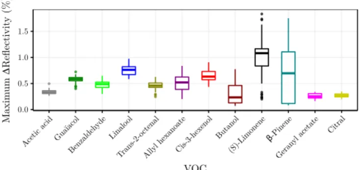
Figure 6: Distribution of the maximum intensities over the laps for each VOC.

R2_r equals the proportion of variance explained by the model compared to the total variance in Yr. The values of R2rfor each VOC are reported in Figure 5b and show a generally good fit for all of the VOCs.

5.2. Analysis of the dictionary

The method proposed in this paper is based on a pe-nalised linear regression. A linear regression can suffer from collinearities or multicollinearites which may exist between the signatures of the matrix K ∈ RP ×R_{. A} mul-ticollinearity is present when one column of K is equal

to a linear combination of the other colums. For

non-penalised linear regression, it is easy to show that mul-ticollinearity will cause problems. Indeed, in this case, the classical least-squares solution of y = Kc is ˆc = (KTK)−1KTy. The inversion of KTK requires that

rank(KTK) = rank(K) = R (assuming P > R). This

condition is then violated if there exists at least one mul-ticollinearity.

To check for multicollinearity, we use a well-known in-dicator, namely the Variance Inflation Factor (VIF) (James et al., 2013). Considering a signature kr∈ RP:

VIFr= P p(kp,r− ¯kr)2 P p(kp,r− ˆkp,r)2 (9)

with ˆkr= α0−P_i6=rαiki and ¯krthe mean of kr. Like the R2 _{criterion (eq. (8)), the VIF is dependent} on the notion of variance explained. Here, we regress kr against the other signatures and the greater the VIF is, the more kr is linearly dependent on the other signatures. A VIF equals 1 if and only if kris linearly independent from the other signatures. A classical rule is that a VIF which is greater than 5 or 10 indicates collinearity problems (James et al., 2013).

To illustrate the collinearity problem in our case, we focus on a smaller dictionary which will be used for Setup 2. The results are reported in Table 2. From the Table 2, the factors indicate strong collinearities between the sig-natures even with only 4 VOCs in the dictionary (for the complete dictionary, the results are even worse). These results motivate the use of Algorithm 2 and its `1-penalty which can help to combat these multicollinearities. 5.3. Cross-validation

In order to avoid an overestimation of the score (with the criterion defined in Section 4.2), we perform a cross-validation. In fact, if we extract the signatures with all 28 laps and then predict the labels for these same laps, we may introduce a bias as the training set (extraction of the signatures) is then the same as the testing set.

To perform cross-validation, we divide the 28 laps into β folds (here, β = 5). The laps corresponding to the first β − 1 folds are taken for extracting the dictionary and the βth fold is used for testing. Concretely, for the testing laps, we apply Algorithm (2) which returns an intensity vector c(t) for a measurement vector y(t). From this in-tensity vector, we extract a label for each region of interest which has been previously identified with a segmentation step (see Supplementary Materials). We then repeat the procedure for all the β folds and compute the classifica-tion rate and the confusion matrix. Finally, we repeat the entire cross-validation 10 times with new folds. From these 10 cross-validations, the classification rates and the confusion matrices are averaged.

5.4. Results

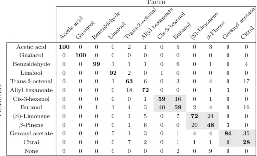
The confusion matrix is reported in Table 3 and the average classification score is 73.7 ± 21.9 % which is much larger than the chance level (8.33%). Despite the difficulty of the task, some VOCs are even perfectly or almost per-fectly identified. It means that almost all the gas sources containing these VOCs have been correctly recognised (e.g. Acetic acid or Benzaldehyde). However, it happens that Algorithm 2 does not find any VOC (i.e. all the VOCs have a null intensity) even if the segmentation does. These estimations have been classified as “None” in the confu-sion matrix and correspond to regions of interest with low signal to noise ratio. For these regions, the null solution must have the lower cost compared to solutions with one or more VOCs.

Figure 6 represents the distribution of the maximum intensities for each VOC over the time. The diversity of intensities is clear, showing the exhaustion of some VOCs (e.g. β-Pinene) and the stability of others (e.g. Gua¨ıacol). It demonstrates that the good classification score cannot be attributed to a single factor such as a simple difference of intensity between VOCs. Recognition performance can only be explained by the variability in affinities between the sensing materials and the VOCs that produces recog-nisable signatures.

Truth Acetic acid Gua ¨ıacol Benzaldeh yde Linalo ol Trans-2-o ctenal Allyl hexanoate

Cis-3-hexenolButanol (S)-Limoneneβ-PineneGeran ylacetate Citral Prediction Acetic acid 100 0 0 0 2 1 0 5 0 3 0 0 Gua¨ıacol 0 100 0 0 0 0 0 0 0 0 0 0 Benzaldehyde 0 0 99 1 1 1 0 6 0 1 0 4 Linalool 0 0 0 92 2 0 1 0 0 0 0 0 Trans-2-octenal 0 0 0 1 63 6 0 3 0 4 0 17 Allyl hexanoate 0 0 0 0 18 72 0 0 0 1 3 0 Cis-3-hexenol 0 0 0 0 0 1 59 16 0 1 0 0 Butanol 0 0 1 1 4 3 40 59 2 4 0 16 (S)-Limonene 0 0 0 0 1 5 0 7 72 24 9 0 β-Pinene 0 0 0 0 1 6 0 0 20 48 3 0 Geranyl acetate 0 0 0 5 1 3 0 1 4 4 84 35 Citral 0 0 0 0 7 2 0 1 1 1 0 28 None 0 0 0 0 0 0 0 2 0 9 0 0

Table 3: Confusion matrix for the data from Setup 1. The colored cells correspond to pairs of VOCs which are hard to differentiate. A None class has been added when Algorithm (2) did not find any VOC. In fact, it happens that for some regions of interest, Algorithm (2) does not find any VOC (all the intensities are null) whereas the segmentation method did not discard them (especially areas with low signal to noise ratio).

Misclassifications are sometimes due to the fact that some pairs of VOCs are quite hard to differentiate (col-ored cells in Table 3). It is interesting to note that these pairs are sometimes from the same chemical family. For instance (Butanol, Cis-3-Hexenol) are both Alcohols and (β-Pinene, (S)-Limonene) are both Alcenes and they even share the same molar mass. Of course, chemical similarity is not the whole story, since e.g. Linalool is not confused with other Alcohols. The misclassifications between Cit-ral and Geranyl acetate can be attributed to the lower to-noise ratio for these two VOCs. This low signal-to-noise ratio can be explained by both their low volatility and their low affinity with the sensing materials.

6. Gas unmixing

In this section, we tackle the issue of gas unmixing with the data from Setup 2 (see Section 3.2.2). We remind the reader that we have generated various realistic scenarios with increasing complexity: _{¬ the gas sources are isolated} and spatially close, _{­ the gas sources are successive trails} of pure compounds and _{® the gas sources are successive} trails of binary compounds. In each scenario, the data correspond to 20 sweeps (from left to right, the results for the other direction is in the Supplementary Materials). Each one of these 20 sweeps is then processed separately for the unmixing with the previously generated dictionary and with Algorithm 2.

In the following, when considering a measurement y(t), we assume that baseline drift has been subtracted using Algorithm (1).

6.1. Building and pruning of the dictionary

The dictionary K ∈ RP ×R is built with the method

detailed in Section 5.1 and from the whole data set from Setup 1. This last point is an important aspect of the following results: it implies that the training setup is not the same as the testing setup. This characteristic is quite important in practice. Indeed, the dictionary will be al-ways generated in a separated setup in order to be used in the field afterwards. So, training with Setup 1 and testing with Setup 2 will assess the robustness of the proposed method.

From the dictionary, we first extract the set of the 4 VOCs which are present in the scenarios_{¬ to ®, namely:} Citral, (S)-Limonene, Gua¨ıacol and Cis-3-hexenol. At least one VOC is always used as a control, meaning that at least one VOC is present in the dictionary but not in the ex-periment. We call the VOCs actually present the target VOCs. We expect that the estimated intensity of the con-trol VOC will be close to or equal to 0. This is a key point of our results; indeed, an eNose is a non-specific device that can generate signatures for a broad variety of VOCs, contrary to specific sensors which are designed for one or two VOCs. In practice, an eNose may be less effective than specialised sensors if we only target 2 specific VOCs. So there is no reason to favour an eNose except if we want to use it for a large amount of applications with a lot of different VOCs. That is why, in practice, the dictionary will be as large as possible and only an unknown subset of VOCs from the dictionary will be relevant for a given application. To our knowledge, by considering a larger dictionary than the number of VOCs actually present, we go further than most of the studies in the field and

es-Citral (S)-Limonene Distance

Source 1 Source 2 Source 1 Source 2 Source 1 Source 2

Mean ± Standard deviation (cm) 8.6 ± 0.35 27.9 ± 0.50 11.9 ± 0.31 25.5 ± 0.28 3.3 ± 0.41 2.3 ± 0.47

Ground-truth (cm) [8,8.5] [27,27.5] [11.5,12] [25.5,26] 3 1

Table 4: Estimation of the position of the isolated gas sources from Scenario¬ with the default dictionary (Citral, (S)-Limonene, Gua¨ıacol,

Cis-3-hexenol), based on the maximum intensity. The column distance refers to the spatial distance between Citral and (S)-Limonene.

pecially studies which perform mixtures-learning. What’s more, these 4 VOCs are clearly not the best subset of the 12 VOCs from Setup 1. Indeed, by looking at the confu-sion matrix in Table 3, the subset containing Acetic acid, Gua¨ıacol, Benzaldehyde and Linalool would probably lead to much better results than the ones presented here.

The results with the dictionary of 4 VOCs are described in the next section. Afterwards, we progressively extend the dictionary by adding one VOC at a time. The order of the VOCs is defined with the help of the confusion matrix

(Table 3). Given the current set of VOCs in the

sub-dictionary, we simply add all the confusions made with these VOCs (i.e. we add amongst themselves the columns

of the confusion matrix containing the set). Then, we

take as new member of the set the VOC which has the lowest confusion coefficient. With this method, the order of the VOCs (after the 4 VOCs already chosen by default) is: Acetic Acid, Allyl-hexanoate, Linalool, Benzaldehyde, Trans-2-octenal, β-Pinene, Geranyl acetate and Butanol. The task is then harder and harder and, at the end, the whole dictionary is used in the unmixing.

6.2. Results with a dictionary of 4 VOCs

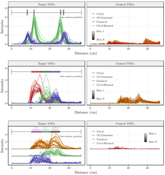
The intensities estimated for the 4 VOCs in the 3 sce-narios are represented in Figure 7. Each color stands for a VOC and each line corresponds to a sweep (a color gra-dation indicates the sweep index).

For Scenario _{¬, the intensities are reported in the} top panel of Figure 7. The intensities of Citral and (S)-Limonene clearly indicate good unmixing from the sig-nals previously shown in Figure 3b. We can notice that the intensities of the controls (namely Cis-3-hexenol and Gua¨ıacol) are not strictly null. However, these intensi-ties correspond mainly to transition areas (from one gas source to another) or to areas with low signal to noise ra-tio (SNR). What’s more, the intensities of the controls are much lower than the intensities of the two VOCs actually present. By computing the classification criterion defined in Section 4.2, we reach a noteworthy score of 90% (98% for the other direction) for the spatial areas defined by the scent strips (corresponding to a total of 240 measure-ments). In this scenario, we even go further by estimating the spatial position of each isolated gas source. For that, we simply take as the position of a gas source, the position of its maximum intensity. The average estimated intensi-ties for the 20 sweeps are reported in Table 4. These re-sults highlight a good estimation of the position of the gas

sources when they are far enough from each other (sep-arated by 3cm). The same task is harder for a smaller distance (1cm) for which the distance is overestimated. In addition, (S)-Limonene presents better estimation results compared to Citral. This can be explained by the possi-ble lags introduced in Section 4.2, especially the chemical lag and the lag related to the airflow. Indeed, Citral is a heavier molecule than (S)-Limonene (see Table 1) so its transport and its interaction with the chemical sensors can take more time and thus delay the measurement.

For Scenario_{­, the results are represented in the} mid-dle panel of Figure 7. Again, the estimated intensities cor-respond to the spatial areas of the gas sources. However, the estimated intensity of the control (here, Cis-3-hexenol) is no more negligible and no more restricted to low-SNR re-gions. We notice that the intensity of the control VOC de-pends mainly on the VOC present. Indeed, the gas source containing Gua¨ıacol is well estimated whereas the estima-tions for the other gas sources ((S)-Limonene and Citral) are more affected by Cis-3-hexenol. This observation is a consequence of the existence of linear dependencies be-tween the signatures. Despite these correlations, we find a classification score of 83% (92% for the other direction), out of 1 520 measurements. This score is quite good in view of the difficulty of the task. Even if the intensity of the control VOC is high, it is still lower than those of the target VOCs.

Finally, for Scenario _{®, the intensities are reported} on the bottom panel of Figure 7. At first sight, the re-sults seem better than for Scenario _{­ which is simpler,} especially if we focus on the control VOC. In fact, the control VOC is no more Cis-3-hexenol but now Gua¨ıacol. Gua¨ıacol seems to be a much better control VOC than Cis-3-hexenol. Indeed, the estimated intensities of Gua¨ıacol are close to 0, as expected. This can be explained by a VIF which is lower for Gua¨ıacol (see Table 2) and by the Table 3 which shows that Gua¨ıcaol is perfectly identified despite the 11 other VOCs. For the present VOCs, the es-timated intensities match with the spatial position of the gas sources, especially for the gas sources containing Cit-ral and (S)-Limonene. The intensities of Cis-3-hexenol are less simple to analyse since the intensities exceed the spa-tial areas of its gas sources which could be due to ternary mixtures. However, a comforting fact is that these intensi-ties clearly decrease when the eNose goes over a gas source which does not contain Cis-3-hexenol. The score reaches

Target VOCs Control VOCs 0 10 20 30 0 10 20 30 0 2 4 6 Distance (cm) In tensit

y Gas sources position

Citral (S)-Limonene Guaïacol Cis-3-Hexenol Run 1 Run N

Target VOCs Control VOCs

0 10 20 30 0 10 20 30 0 2 4 6 8 Distance (cm) In tensit

y Gas sources position

Citral (S)-Limonene Guaïacol Cis-3-Hexenol Run 1 Run N

Target VOCs Control VOCs

0 10 20 30 0 10 20 30 0 2 4 Distance (cm) In tensit y Citral Cis-3-Hexenol Citral (S)-Limonene Cis-3-Hexenol (S)-Limonene

Gas sources position

Citral (S)-Limonene Guaïacol Cis-3-Hexenol Run 1 Run N

Figure 7: Results of the proposed algorithm for the different scenarios introduced in Section 3.2.2. Each line corresponds to one sweep (first sweep is the lighter). Each color corresponds to the estimated intensity of the given VOC at the distance d. The results have been generated

with the default dictionary ((S)-Limonene, Citral, Gua¨ıacol, Cis-3-hexenol). For Scenario®, the intensities of Citral and (S)-Limonene have

been vertically shifted for easier visualisation.

72% (71% in the other sweep direction) which means that the identity of 72% of all binary mixtures (corresponding to 1,520 measurements, i.e. 1,520 mixtures) has been well predicted.

6.3. Results with a dictionary of increasing size

The previous results emphasize that we can achieve good classification performance even with one or two VOCs which are not present in the experiment but present in the

dictionary. Here, we go even further by adding one-by-one each VOC from the full dictionary. As a reminder (see Sec-tion 6.1 for details), the order according which the VOCs are added, is the following: Acetic acid, Allyl-hexanoate, Linalool, Benzaldehyde, Trans-2-octenal, β-Pinene, Ger-anyl acetate and Butanol.

Concretely, we start by adding the signature of Acetic acid to the previous dictionary of size R = 4 ((S)-Limonene, Citral, Gua¨ıacol, Cis-3-hexenol). Then, we apply

Algo-90 % 89 %

72 %

1 2 3

1 - Close isolated sources 2 - Successive pure trails 3 - Successive binary trails

+ Butanol + Geran yl acetate + β-Pinene + T rans-2-octenal + Benzal. + Linalo ol + Allyl hexanoate + A cetic acid Default

Spatial distribution of the classification score Average score

Num ber of V OCs R in the dictionary 4 5 0 10 20 30 0 10 20 30 0 10 20 30 R = 2 R R = 3 R R = 3 R Distance (cm) No groundtruth

Citral (S)-Limonene (S)-Limonene Citral Guaïacol Citral

(S)-Limonene

Citral

Cis-3-hexenol (S)-LimoneneCis-3-hexenol

(S)-Limonene Citral Best dictionary {Citral,(S)-Limonene} 0 50 100 Score (%)

Figure 8: Influence of the size of the dictionary on unmixing performance. From the bottom up, the number of VOCs in the dictionary is increasing, starting from the default dictionary ((S)-Limonene, Citral, Gua¨ıacol, Cis-3-hexenol). Left to right, the three first left panels correspond to the spatial distribution of the score for each scenario (for a position d, the score is the average across the 20 sweeps). The

spatial distribution highlights the misclassifications (mainly in transition areas) in each scenario and for each dictionary. For Scenarios­

and®, a black line indicates the transitions between one gas source to another. Finally, the right hand panels correspond to the average score

in each scenario and for each dictionary (averaging over space and across the two sweeps). For each individual panel, the left bar corresponds to the score of the best dictionary (i.e. the smallest) and the right bar correspond to the score of the current dictionary.

rithm (2) to unmix the signals and estimate the intensity of each VOC of this new sub-dictionary. Ideally, the es-timated intensity of Acetic acid is close to 0. However, in practice the new VOC could considerably disrupt the unmixing, especially due to correlations which may ex-ist between this new signature and the signatures already present. To assess the influence of this new VOC, we sim-ply generate the label `(t) based on the maximum intensity of c(t) (see Section 4.2 for details). This predicted label is then compared to the position of the gas sources. In Fig-ure 8, we report both the spatial distribution of the errors averaged across the sweeps (left panel) and the average score (right panel). Afterwards, we repeat the procedure by adding Allyl-hexanoate and so forth for the others.

Un-til we reach the upper limit of R = 12 VOCs (the full dic-tionary), the task becomes harder and harder with each new VOC we add.

From Figure 8, for Scenarios _{¬ and ­, we see that}

the scores start to considerably decrease only at R = 10 VOCs. It is noteworthy that even with 9 VOCs in the dictionary, we can reach a classification score of 88% for

Scenario _{¬ and 76% for Scenario ­. In fact, R = 10}

corresponds to the addition of β-Pinene which is highly-correlated (99.8 %) to (S)-Limonene (for the two scenarios, the gas sources of (S)-Limonene are no longer identified). Afterwards, at R = 11, the addition of Geranyl acetate produces another large decrease of the scores (again, for the two scenarios, the gas sources of Citral are no longer