An advanced discrete fracture model for variably saturated flow in fractured porous media

HAL Id: hal-02890324

https://hal.inrae.fr/hal-02890324

Submitted on 9 Dec 2020

HAL is a multi-disciplinary open access archive for the deposit and dissemination of sci-entific research documents, whether they are pub-lished or not. The documents may come from teaching and research institutions in France or abroad, or from public or private research centers.

L’archive ouverte pluridisciplinaire HAL, est destinée au dépôt et à la diffusion de documents scientifiques de niveau recherche, publiés ou non, émanant des établissements d’enseignement et de recherche français ou étrangers, des laboratoires publics ou privés.

An advanced discrete fracture model for variably

saturated flow in fractured porous media

Behshad Koohbor, Marwan Fahs, Hussein Hoteit, Joanna Doummar, Anis

Younes, Benjamin Belfort

To cite this version:

Behshad Koohbor, Marwan Fahs, Hussein Hoteit, Joanna Doummar, Anis Younes, et al.. An advanced discrete fracture model for variably saturated flow in fractured porous media. Advances in Water Resources, Elsevier, 2020, 140, �10.1016/j.advwatres.2020.103602�. �hal-02890324�

An advanced discrete fracture model for variably saturated flow in

fractured porous media

Behshad Koohbor1, Marwan Fahs1*, Hussein Hoteit2, Joanna Doummar3, Anis Younes1,4,5,

Benjamin Belfort1

1_{Laboratoire d’Hydrologie et Géochimie de Strasbourg, Université de}

Strasbourg/EOST/ENGEES, CNRS, 1 rue Blessig 67084 Strasbourg, France.

2

Physical Science and Engineering Division, King Abdullah University of Science and Technology (KAUST), Thuwal, Saudi Arabia

3

Department of Geology, American University of Beirut, Beirut, Lebanon

4

IRD UMR LISAH, F-92761 Montpellier, France.

5

Laboratoire de Modélisation en Hydraulique et Environnement, Ecole Nationale d’Ingénieurs de Tunis, Tunisia

Received 17 February 2020; Received in revised form 10 April 2020; Accepted 24 April 2020 Available online 6 May 2020

Koohbor, B., Fahs, M., Hoteit, H., Doummar, J., Younes, A., & Belfort, B. (2020). An advanced discrete fracture model for variably saturated flow in fractured porous media. Advances in Water Resources, 103602. https://doi.org/10.1016/j.advwatres.2020.103602

*Contact person: Marwan Fahs // E-mail: fahs@unistra.fr

Keywords: Variably saturated flow; Fractured Porous media; Discrete fracture model; Mass

Abstract

Accurate modelling of variably saturated flow (VSF) in fractured porous media with the discrete fracture model (DFM) is a computationally challenging problem. The applicability of DFM to VSF in real studies at large space and time scales is somewhat limited not only because it requires detailed information about the fractures, but also as it involves prohibitive computational efforts. We develop an efficient numerical scheme to solve the Richards’ equation in discretly fractured porous media. This scheme combines the mixed hybrid finite element method for space discretization to the method of lines for time integration in order to improve the capacity to deal with real field applications. The fractures are modeled as lower dimensional interfaces (1D), embeded in 2D porous matrix. A new mass lumping (ML) technique has also been provided for the fractures to avoid unphysicall oscillations that can lead to convergence issues. The new developed scheme is implemented in a numerical code which is validated against COMSOL Multiphysics for a problem involving water table rechage at laboratory scale. Computaional efficiency of the developed numerical scheme is hilighted using the challenging problem of water infitration in fractured dry soil and by comparison against standard numerical techniques used in exisiting codes. ML-technique for fractures allows for a significant gain in CPU time. The new developed code is used to investigate the effect of climate change on groundwater ressources in a karst aquifer/spring system in El Assal, Lebanon. Simualtions tacking into account predicted recharge under climate change are carried out for about 80 years, up to 2099. This application serves as showcase of the applicability of the developed numerical scheme to deal with real cases involving large time and space scales and variable recharge. The proposed scheme shows high robustness and computational performance. The results indicate that neglecting fracutres leads to an overstimation of the amount of available groundwater. The level of water table is sligthly sensitive to fractures. The developed scheme is generic and has a comprehensive perspective in practice. It can be implemented in any finite element-based methods and can be extended to 3D.

1. Introduction

Understanding variably saturated flow (VSF) in fractured porous media has great significance to many environmental and geotechnical applications, such as groundwater recharge in karst aquifers, (Mudarra and Andreo, 2011; de Rooij et al., 2013 de Rooij, 2019), epikarst (Chang et al. 2019) and unconfined chalk aquifers (Ireson et al, 2009), geological disposal of nuclear waste such as at Yucca Mountain in the United States where the unsaturated zone is estimated as potential site for disposal of high-level nuclear waste (Hayden et al., 2012; Ye et al., 2007), contaminant transport and infiltration of landfill leachate (Brouyère, 2006; Ben Abdelghani et al., 2015), infiltration through unsaturated saprock in hillslopes with shallow fractured shale bedrock (Guo et al., 2019), unsaturated flow and contaminant transport in saprolite (Van der Hoven et al., 2003; Alazard et al., 2016), water flow in cracked soils and stability of soil slopes with cracks (Pouya et al., 2013; Wang at al., 2019; Yang and Liu, 2020), seepage through fissured dams (Jiang et al., 2014), tunnel excavation (Gokdemir et al., 2019) and protection of structure foundations in contact with water (Zhao et al. 2019).

The fractures in the vadose zone can serve as preferential flow pathways, but they could also form capillary barriers, depending on the degree of saturation (Cey et al., 2006; Wang and Narasimhan, 1985). The VSF in fractured porous media involves several coupled and complex processes such as capillary and gravity-driven transient flows, preferential flow in fractures, fracture-matrix interactions and matrix diffusion. Due to these complexities, and despite the wide range of applications, the processes of VSF in fractured porous media remains not well-understood, relatively to saturated flow. Related experimental studies are scarce and limited to simplified configurations (e.g. one simple fracture or simple fracture intersections). For instance, Yang et al. (2019) presented an experimental study to investigate VSF through simple T-shaped fracture intersection. Wang et al. (2017) investigated the effect of fracture aperture on capillary pressure-saturation relation. Kordilla et al. (2017) studied the

effect of droplet and rivulet unsaturated flow modes at simple fracture intersection. Based on experiments, Tokunaga and Wan (2001) introduced a new mechanism of VSF in one simple fractured domain called “surface-zone flow" which can appear when the permeability of skin fractures is significantly greater than that of matrix.

Most of the studies related to VSF in fractured domains rely on numerical simulations which are used for several theoretical and practical purposes as, for instance, understanding physical processes (Liu et al., 2002, 2004), field studies (Zhou et al., 2006; Ye et al., 2007; Masciopinto and Caputo, 2011; Kordilla et al., 2012; Ben Abdelghani et al., 2015; Robineau et al., 2018) and validation of laboratory experiments (Roels et al., 2003; Malenica et al., 2018). In applied studies numerical simulations are considered as an irreplaceable and cost-effective tool for designing, predicting, and uncertainty assessments. Usually unsaturated flow is described using the Richards’ equation (RE) that combines Darcy’s law and continuity equation which are coupled via constitutive relations expressing permeability and water content as function of hydraulic head (Farthing and Ogden, 2017). RE is a simplification of the two-phase (water-air) flow model assuming that air remains essentially at atmospheric pressure. It has been shown to be a good approximation of unsaturated flow when the effect of the air on water flow in negligible (Szymkiewicz, 2013). Furthermore, the models used to treat the fractures can be classified in two main categories: the equivalent continuum model (ECM) and the discrete fracture model (DFM). With the ECM, the fractured domain is replaced by a homogenous porous media with equivalent hydraulic parameters. In this case, RE is used with specific permeability constitutive relation and retention curve including the effect of fractures. The main research on the ECM are devoted to the development of effective retention and permeability curves in the presence of fractures (Guarracino and Quintana, 2009; Monachesi and Guarracino, 2011; Pouya et al., 2013). The dual porosity model, which can be seen as an improvement of the ECM, treats the fractured domains as dual interactive

continua representing fractures and porous matrix, respectively (Brouyère, 2006; Kuráž, 2010). Different hydraulic properties are associated to each continuum. Flow cannot occur in the matrix continuum that acts as a source/sink for water imbibition while the fracture continuum is highly permeable with low storage capacity (Fahs et al., 2014). Dual permeability model is more used than dual porosity for VSF in fractured domains as it allows for considering moisture flow in both fracture and matrix continua (Kordilla et al., 2012; Robineau et al., 2018). Dual permeability model requires two sets of constitutive relations for the fracture and matrix domains, respectively. While in the ECM the fractures are implicitly presented, the DFM is based on an explicit description of fractures. Hydraulic properties of fractures and their topology are explicitly considered and the porous matrix and the fractures are simulated as separate elements of one continuum. For DFM, RE is often borrowed to simulate flow in both fractures and porous matrix, but with different constitutive relations and properties for each compartment. Examples of utilization of the DFM for VSF can be found in

Therrien and Sudicky (1996), Masciopinto and Caputo (2011), Ben Abdelghani et al. (2015), Li and Li (2019) and Li et al. (2020).

ECM provides efficient simulations with relatively low computational costs and complexity. It is relatively simple and straightforward to implement. This is why ECM is commonly used in real field applications (Liu et al., 2005). However, robustness of this model is highly depending on the capacity of the equivalent retention curves and constitutive relations in presenting the porous matrix and the fractures (Liu et al., 2005). ECM is not appropriate for small scale applications or for cases involving small number of fractures (Roels et al., 2003). Due to the assumption of equivalent porous media, ECM is unable to provide detailed description of the flow dynamics in fractures and fails to reproduce the preferential flow paths encountered in fractured vadose zone (Liu et al., 2005, 2007). DFM is more suitable to simulate preferential flow as fractures are considered in great details. This model is essential

to understand water flow processes in fractures at small scale (Cey et al., 2006). It is also applied for field scale with small numbers of well-defined fractures (Hirthe and Graf, 2015; Ben Abdelghani et al., 2015). However, DFM is computationally expensive and requires detailed information about fractures. It is more complex for implementation than ECM. It requires dense computational meshes and suffers from poor convergence due to the high discontinuity between the hydraulic properties of fractures and matrix, particularly in the case of dense fracture networks (Berre et al., 2019; Nordbotten et al., 2019). A common approach that significantly alleviates the computational complexity of the DFM is the hybrid-dimensional technique (Therrien and Sudicky, 1996; Hoteit and Firoozabadi, 2008; Li et al., 2020) in which the fractures are considered as co-dimensional interfaces with respect to the full-dimensional elements representing the porous matrix (i.e. one-dimensional fractures embedded in two-dimensional porous matrix elements).

Recently, with the continued advancement in new numerical methods and the progresses in powerful computational technologies, the DFM model has received an increasing interest due to its robustness in reproducing physical processes of flow and transport in fractured porous media. This results in extensive research on the development of appropriate numerical techniques and schemes that aims at improving the computational performance of the DFM (Ahmed et al., 2017; Berre et al., 2019; Nordbotten et al., 2019). This study focuses on the use of the DFM for the simulation of water flow in vadose fractured zones.

Modeling VSF in explicitly fractured domains (i.e. with the DFM) remains a computationally challenging task which is usually struggles with numerical complexities (Li and Li, 2019). It is challenging because of massive fractures and the associated complex geometry, highly discontinuities, mesh discretization requirement and poor resulting convergence but also due to the inherent numerical complexities of the RE (Li and Li, 2019). In fact, it is well-known that the numerical solution of the RE, even in non-fractured domains, is one of the most

challenging problem in hydrogeology (Miller et al., 2013). Numerical difficulties are caused by the mathematical characteristics of this equation that could change from hyperbolic to parabolic depending on the saturation and by the strong nonlinearity introduced by the constitutive relationships (Suk and Park, 2019). Convergence issues, small time step size, mass conservation and numerical oscillations are common numerical problems usually encountered in the solutions of RE. This is why significant efforts have been made in last decades on the development of advanced and appropriate numerical techniques for solving this equation (i.e. Celia et al., 1990; Farthing et al., 2003; Li et al., 2007; Ji et al., 2008; Fahs et al., 2009; Hassane Maina and Ackerer, 2017; Suk and Park, 2019; Ngo-Cong et al., 2020). The most addressed questions are the choice of the primary variable (pressure head, water content or mixed form), mass conservative solution, spatial discretization, time discretization and time step management, nonlinear solvers and numerical evaluation of equivalent hydraulic conductivity (Miller et al., 2013 and references therein). More details about the numerical solution of RE can be found in both recent review papers by Farthing and Ogden (2017) and Zha et al. (2019).

In contrast, to the non-fractured domain, the numerical solution of RE in explicitly fractured domains (i.e. with the DFM) are still not well-developed. Most of the existing tools are based on standard numerical techniques, i.e. standard finite element method for space discretization and backward Euler scheme for time integration (Therrien and Sudick 1996), that are not well suitable to solve this equation under complex fractured configurations. This restricts the applicability of existing models for engineering practice, especially at real scale. It is clear that accurate and fast solutions of RE in explicitly fractured domains is beyond the capabilities of current numerical models. Hence, it is important to carry out further studies on the development of robust and efficient numerical techniques to solve the RE in explicitly fractured domains involving complex fracture network, which is the main objective of this

study. This is crucial to improve the capacity of current models in developing more realistic simulations and to deal with the growing demand on predicting and understanding the dynamics of aquifers under non-stationary conditions, at large time and space scales as, for example, in climate change studies. The objective of this paper is to develop a new numerical technique for VSF in fractured porous domains that is not only accurate but also efficient and fast, which is a fundamental challenge of computation water resources.

Thus, we couple most updated and appropriate numerical techniques for space discretization and time integration in order to solve the RE in explicitly fractured domains. We consider the head-form of the RE. This form allows for simplifying numerical solution as only the pressure-head is used as primary variable. However, it can lead to non-conservative solutions when it is solved with first order time integration methods (Celia et al., 1990; Farthing et al. 2003). To avoid this problem and to obtain conservative solutions, we use high order integration technique, as it is discussed further in this section. Among different existing techniques for space discretization of the Darcy’s law, we use the mixed hybrid finite element (MHFE) method (Brezzi and Fortin, 1991; Farhloul and Fortin, 2002; Farhloul, 2020). A review about the use of this method and its advantages (e.g. local mass conservation, ability to intrinsically treat anisotropic domains, consistent velocity field even in highly heterogeneous domains) in simulating groundwater flow can be found in Younes et al., (2010). MHFE has been initially used to simulate saturated flow in simple porous media (Younes et al., 1999). It has been then extended to VSF by Farthing et al. (2003), Fahs et al. (2009) and Belfort et al. (2009). As the method deals with the water fluxes and average pressures at the edges of the mesh elements, it is highly suitable for the DFM with the hybrid-dimensional technique where fractures are defined on the edges of the matrix elements. The method has been extended to the simulation of flow in saturated fractured porous media in Hoteit and Firoozabadi (2008),

(2017). For VSF, the MHFE has been only applied to non-fractured domains. One of the objective of this work is to extend this method to VSF in explicitly fractured domains and to evaluate its performance in such an application. An important task in this aim is the development of an appropriate mass lumping (ML) technique. In fact, as the nonlinearity of the RE imposes small time step size, any finite-element based method could suffer from spurious oscillations related to the discretization of the transient accumulation term (Elguedj et al., 2009; Scudeler et al., 2016). This problem has been encountered with the MHFE in

Belfort et al. (2009). For RE the problem of unphysical oscillations is particularly crucial as it leads to a loss of numerical stability that would affect the convergence of the nonlinear solver.

Younes et al. (2006) developed a ML technique for the MHFE to damp the unphysical oscillations. Belfort et al. (2009) extended the ML technique to VSF in non-fractured domains. In this work we develop an efficient way to generalize the ML technique to VSF in fractured domains. Finally, in general, little attention has been devoted to the time integration of ground water flow in fractured domains (Moortgat et al., 2016). This is also true for VSF with the DFM. Existing numerical models are based on the first-order backward Euler scheme (Therrien and Sudick 1996). However, several works show the advantages of higher order time integration schemes for the simulation of unsaturated flow. Farthing et al. (2003) showed that with higher order time integration scheme, conservative solutions can be obtained even with the non-conservative form of the RE. Fahs et al. (2009) proved that adaptive high order time integration schemes can lead to faster solutions than standard first order method. Here we couple the MHFE and the ML technique to an adaptive high order time integration scheme via the method of lines (MOL) (Matthews et al., 2004). This permits for using a sophisticated ordinary differential equation (ODE) solver for time integration (DLSODIS) that allows, beside high order adaptive time integration, an appropriate time stepping management and efficient procedure to deal with nonlinearities.

2. Governing Equations of VSF in fractured domains

VSF in both fractures and porous matrix is described by the RE coupling the Darcy-Buckingham’s law and the mass conservation equation, as shown below:



_e ( )



q  K S h  H (1)



c h( ) S S_{s w} ( )



H .q f t    _  

_

  _{ }  _   (2) H h z (3)

Where superscript 



M F,



is the medium index (M for porous matrix and F for fracture),

Hβ [L] and hβ [L] are, respectively, the piezometric head and pressure head, and z [L] is the elevation. The list of variables and parameters associated with Eqs. (1) and (2) are provided in Table 1.

Table 1. The definition of parameters and variables associated with the governing equations

Parameter Definition Dimension

K hydraulic conductivity _L T. 1_ r e s r S        effective saturation [ ]



water content [ ] r



residual water content [ ] s



saturated water content [ ] s

S

specific storage _L1_ w s S





 relative saturation [ ]

 

d c h dh 

 specific moisture capacity _L1_

For both fractures and porous matrix, we use the standard form of the van Genuchten (1980)

model for the inter-relation of pressure head and water content. Different properties are considered for porous matrix and fractures:





1 0 1 | | 1 0 m n r e s r h S h h                  _   _{ }  _  _  _     (4)

Where αβ [L-1] and n [-] are parameters related to the mean pore size and uniformity of mean size distribution of the porous matrix and fractures, and m 1 1

n





  . For conductivity-saturation relationship, the van Genuchten - Mualem’s model (Mualem, 1976)is given by:

 

 

1/ 2

1

1

m m s e e

K

K

S

S

  

_

 



_

_{ }









_







_

_







(5)

3. Numerical solution: MHFE method, ML technique and MOL

A new numerical scheme is developed to solve the system of Eqs. (1)-(5). The new scheme is developed for 2D unstructured triangular meshes, but it can also process with any type of mesh. As mentioned in the introduction, the fractures are considered with the hybrid-dimensional technique (1D interfaces of the 2D elements representing the porous matrix) which allows significant reduction in the computational mesh complexity. The new developed scheme couples the MHFE and ML technique for space discretization with and advanced ODE solver for time integration via the MOL. This method consists in discretizing the space derivatives while maintaining the time derivative in its continuous form. This allows for converting the system of partial differential equation into a system of ODEs which is solved using a sophisticated solver. The main steps of the developed schemes are detailed here.

3.1 Trial functions of the MHFE method for both porous matrix and fractures

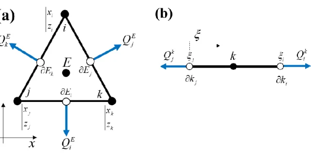
Since the porous matrix and fracture elements have different dimensions, the governing equations are discretized separately, then coupled and solved simultaneously. In the porous matrix, based on the formulation of MHFE, the total flux across edges of an element E, referred to as QE, is approximated as the following (Chavent and Jaffré, 2014) :

1 nf E E E i i i Q Q W  



(6)

Where

Q

_iE is the flux across edge “i” in element E, referred to as ∂Ei. This discretization

technique applies to the porous matrix elements (Fig. 1a) and the fracture interfaces (Fig. 1b). For fracture edges, element E becomes ∂E and edges of the elements becomes the nodes of the fracture edge. We use the lowest order Raviart-Thomas space (Raviart and Thomas, 1977), for which nf is equal to 3 for triangles used for porous matrix elements, and 2 for the fracture edges.

Fig. 1. The fluxes and the used notations for: (a) a porous matrix element and (b) a fracture

The shape functions,

W

_iE for the ith edge of a porous matrix element (E), when using the lowest order Raviart-Thomas space are:

1 , 1, 2, 3 2 | | E E i i E i x x W i E z z             (7)

where | E | [L2] is the surface area of the porous matrix element and

x

iE[L] and E i

z

[L] are, respectively, the horizontal and vertical coordinates of the opposite node to ∂Ei. The shape

functions for the fracture edges are:





1 1, 2 k i i W 

 

 i (8)

where is the length of the fracture edge and



_i[L] is the local coordinates of the opposite element node.

3.2 Flux discretization in the porous matrix elements (MHFE method and ML technique)

Applying the MHFE discretization to Eq. (1) and using the flux expression as in Eq. (6) on a porous matrix element and then rearranging the two sides of the equation, we obtain the following expression of the fluxes (Younes et al., 2006):





3 1 , 1   



 E E E i E ij j j Q M H TH (9)

Where HE [L] and TH_jE [L] are respectively the mean piezometric head in element E and on edge ∂Ej.

1 ,

E ij

M , is the inverse of the local stiffness matrix obtained as followed:

 

1 , E E E E ij i j E M 



W K  W (10)

Using the mass-lumping scheme presented by Younes et al. (2006), the flux on edges of the element E are approximated as followed:





| | 3 3 E E E E S E E E i i i s w Q E dTH Q Q c S S dt     (11)

where

Q

_SE [L2T-1] is the sink/source term imposed on the matrix element E. Q [L_iE 2T-1] is the flux corresponding to the stationary problem without the sink/source term that can only be expressed as a function of alternated local matrix and traces of the piezometric head:

3 , 1 E E i E ij j j Q N TH  



(12)

The local matrix has the following form, with the notations written after:

, , 1 , ,   E i E j  E ij E ij E N   M  (13) 3 1 1 E ,i E ,ij j M    



and 3 1 E E ,i i    



(14)

3.3. Flux discretization on a fracture edge

The formulation of MHFE in the fracture edges “k” is similar to the formulation in the porous matrix elements (seeHoteit and Firoozabadi, 2008). Using the same approach as presented for the discretization in the matrix, fluxes are expressed by the average hydraulic head on the fracture edge and hydraulic head on the fracture nodes (see Fig. 1).





2 1 , 1 k k k i k ij j j Q M H TH  



 (15)

 

1 , k k k k ij i j M 



W K  W (16)

Applying Eq. (15) on Eq. (2) for the fracture edges, the continuity equation treated with a finite volume procedure leads to:





2 1 ( ) ( ) k k k k k k k k s w i S i dH c h S S Q Q dt      



  k f Q (17)

where



and refer to the fracture aperture and length respectively. k S

Q [L2T-1] represents the sink/source term inside the fracture, and k

f

Q [L2T-1] is the matrix–fracture volumetric transfer function, which is explained in the next section.

3.4 Hybridization: mass conservation on edges

Obtaining the global format of the discretized equations requires coupling the flux and piezometric head associated with neighboring elements E and E’ having ∂Ei in common. If

edge ∂Ei is not a fracture, the continuity of flux and piezometric head is imposed:

' ' 0 E E i i E E i i Q Q TH TH       (18)

If ∂Ei coincides with a fracture, the total flux across both sides coming from the adjacent

porous matrix elements defines the transfer function Qk_f, which acts as a sink/source term on the fracture edge. As for the continuity of piezometric heads, the mean heads associated with the matrix edges are equal to the mean head in the fracture element, that is:

' ' E E i i k E E i i Q Q H TH TH        k f Q (19)

For further explanation on the elimination of k f

Q in the final format of the equations, refer to

Hoteit and Firoozabadi (2008).

3.5 The new ML technique for fractures

The global matrix corresponding to the discrete system of equations does not necessarily satisfy the M-matrix conditions which require a non-singular matrix with

m

_ii



0

and

m

ij



0

(Younes et al., 2006; Hoteit, et al., 2002). The M-matrix property ensures respecting the discrete maximum principle; in other words, the solution being exempted from unphysical oscillations. The global matrix obtained by MHFE is symmetric and positive definite but is

not in general an M-matrix. In order to improve the property of our numerical scheme, we use a combination of two mass-lumping techniques; one for porous matrix element, as done in section 3.2 and a new technique that we propose for fracture edges. This proposed mass-lumping scheme applied on the fracture edges ensures the consistency of the M-matrix property for the combined matrix/fracture system.

To explain the mass-lumping scheme for the fracture edges, the global matrix of the discrete system (resulting from the MHFE method) is decomposed into nine submatrices including 6 sub-matrices being pairwise transpose of each other due to the symmetry of the global matrix. The decomposition of the global matrix and different sub-matrices are shown in Fig 2.

Fig. 2. Decomposition of the global matrix into nine sub-matrices

Matrix (A) is composed of the coefficients associated with flux continuity between adjacent porous matrix elements where interfaces are not fractures. This matrix is exactly similar to the one obtained with MHFE in non-fractured domain. As the ML technique is used for porous matrix elements, (A) verifies the properties of M-matrix (Younes et al., 2006). Matrix (B) denotes the coefficients associated with the connectivity of matrix and the edges shared with fractures; all of them are negative or zero (see Eq. (11)). Matrix (C) represents the contribution of fracture nodes on the flux continuity on the non-fractured edges. The coefficients of (C) are all zero due to the fact that there is no flow exchange between the

fracture nodes and matrix edges. Matrix (D) is also an M-matrix (see Eq. (11)), and matrix (E) has all negative or zero components when applying the mass-lumping defined in Eq. (11). However, matrix (F), which corresponds to the connectivity and flow exchange between fracture edges, is not necessarily an M-matrix. To get a global matrix satisfying the M-matrix condition, we propose a numerical integration technique to calculate the stiffness matrix (

1 , k ij M ), as followed:









, 2 0 1 k ij k i j f M d K      

_

  (20) k f

K is the hydraulic conductivity of the fracture element (k). The matrix format of M_{k ij,} is as followed:





























0 0 2 0 0 1 i i i j k k f j i j j d d M K d d                                _{ }  _{   }     









(21)

Calculation of the integrals in each component of the matrix can be approximated numerically. Fig3. can schematically describe the process. In Fig. 3a, the red area represents the integral of the diagonal terms of matrix Mk (Eq. 21). In Fig. 3b, the red area corresponds to

the integral for the off-diagonal terms of the Mk (Eq. 21). With the ML technique in fractures,

the red areas are approximated using the rectangular integration as represented with the blue areas. This would result in zero for the off-diagonal elements of the matrix.

Fig.3. The schematic description of the numerical integration of the integrals of the matrix Mk

(Eq. 21): (a) diagonal terms (𝑚𝑖,𝑖)k and (b) off-diagonal terms (𝑚𝑖,𝑗)k. Red areas represent the

integrals with their analytical expression and blue areas are the corresponding numerical approximation.

Calculating the integral analytically (red surface in Fig. 3) will lead to a stiffness matrix that does not satisfy the M-matrix properties. However, numerical approximation (the blue surface in Fig. 3) leads to the following:

3 2 3 0 1 ₂ 0 2 k k f M K              (22) 1 2 1 0 0 1 k f k K M  _ _   (23)

The process leads to a diagonal stiffness matrix. Hence, sub-matrix (F) satisfies also the M-matrix condition that prevents unphysical oscillations of the solution in each time step. The validity of the results is demonstrated in the following sections.

3.6. High order adaptive time integration

The system of differential equations obtained by coupling the discretized fluxes in the matrix and fracture elements leads to a system of temporal ODEs. In this work, we solve this system using the advanced solver DLSODIS (Double precision Livermore Solver for Ordinary Differential equations – Implicit form and Sparse matrix) which is a public domain solver

differentiation formula (BDF). It has the advantage of using high order time integration scheme. Both variable time step sizes and variable integration orders are used to reach accurate solution within optimized CPU time. The integration order variability makes this solver highly accurate when comparing to conventional constant order solvers. In particularly, for VSF, and as shown in Farthing et al. (2003) and Fahs et al. (2009), high order schemes lead to accurate mass balance even with the non-conservative form of RE. The variability of time step size allows reducing the calculation time and therefore results in exceptional efficiency improvement. The accuracy of DLSODIS is controlled by various tolerances related to the relative and absolute errors, which are fixed to 6

10 in this work. The time step size is changed and adapted periodically by the solver to honor the imposed tolerances. The algebraic nonlinear system resulting from the temporal integration of each time-step is solved using a modified Newton iteration scheme (Radhakrishnan and Hindmarsh, 1993) where the Jacobian matrix is approximated using a finite difference method and a column grouping technique of Curtis et al. (1974).

4. Results: Verification and advantages of the new developed numerical

scheme

4.1. Verifications: Fractured Vauclin test case

The new developed numerical scheme, based on the combination of the MHFE method, ML technique and MOL, has been implemented in a FORTRAN code. The main goal of this section is to verify the correctness of this code. Thus, we consider a computationally simple example in order to avoid numerical artifacts. The example is inspired from the laboratory experiment of Vauclin et al. (1979), dealing with water table recharge. This example is accepted as common benchmark for VSF as it provides reliable experimental data for simplified boundary conditions. The laboratory experiment of Vauclin et al. (1979) deals with non-fractured homogenous soil. We inspired four fractured examples by assuming the same

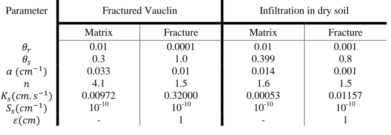
configuration (geometry, dimensions and boundary conditions) and by embedding in the domain i) a single vertical fracture, ii) a single horizontal fracture, iii) a single inclined fracture and iv) a network of fractures similar to networks encountered in karst aquifers. The original experimental setup of Vauclin et al. (1979) consists of a rectangular soil slab (600cm × 200cm). A constant influx of 355 cm/day is applied over a width of 100cm in the center-top of the domain. Initially, the water table is located at 65cm form the bottom surface. Because of the symmetry, only the right half of the domain is considered and the axis of symmetry acts as an impermeable boundary on the left. The rest of boundary and initial conditions are similar to the original experiment. The hydrological properties of the porous matrix are obtained from (Clement et al., 1994), whereas the different fracture properties have been chosen in the ranges provided by different studies (see Fairley et al., 2004; Kuráž et al., 2010; Robinson et al., 2005; Soll and Birdsell, 1998). The matrix and fracture parameters are provided in Table 2. Since the determination of such parameters values for DFM is beyond the scope of the paper, it should be notice that a single kind of fractures has been considered with an emphasis of their high hydrodynamic conduction compared to the soil matrix.

Table 2. Parameters used for the verification examples: Vauclin experiments and infiltration

in dry soil (𝜀 is the fractures aperture).

Parameter Fractured Vauclin Infiltration in dry soil Matrix Fracture Matrix Fracture

𝜃𝑟 0.01 0.0001 0.01 0.001 𝜃𝑠 0.3 1.0 0.399 0.8 𝛼 (𝑐𝑚−1_{) 0.033 0.01 0.014 0.001} 𝑛 4.1 1.5 1.6 1.5 𝐾_𝑠(𝑐𝑚. 𝑠−1_{) 0.00972 0.32000 0.00053 0.01157} 𝑆𝑠(𝑐𝑚−1) 10-10 10-10 10-10 10-10 𝜀(𝑐𝑚) - 1 - 1

The new developed code based on the MHFE method, ML technique (for both fractures and porous matrix) and the hybrid-dimensional technique (1D fractures and 2D porous matrix) is

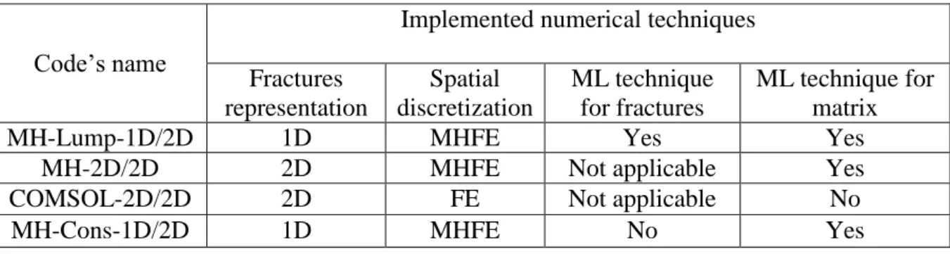
called MH-Lump-1D/2D. It is verified here by comparison against an in-house code based on the MHFE method (with ML technique) and dealing with VSF in non-fractured domains. The in-house code has been validated against experimental data in Fahs et al. (2009). In this in-house code, both porous matrix and fractures are considered as 2D elements. Thus the code is called MH-2D/2D. An example of the difference between the computational mesh used in MH-Lump-1D/2D and MH-2D/2D is given in Fig.4. For more confidence on the correctness of the new developed code (MH-Lump-1D/2D), we compare it against a finite element solution developed using COMSOL Multiphysics. This software provides a tool to simulate fractured porous media based on the hybrid-dimensional technique. But when this tool is used for VSF, the fractures are considered as saturated, which is not the case in our examples. Thus, as in the code MH-2D/2D, we consider the fractures as 2D elements in COMSOL. The COMSOL model is denoted as COMSOL-2D/2D. The numerical codes used for verifications and summary about corresponding numerical techniques are given in table 3. In all codes and in the COMSOL model the time integration is performed in the same manner, using the BDF method with variable order.

Table 3. Specification of different numerical codes used for verifications. (FE: denotes the

standard finite element method). BDF method is used in all codes for time integration.

Code’s name

Implemented numerical techniques Fractures representation Spatial discretization ML technique for fractures ML technique for matrix

MH-Lump-1D/2D 1D MHFE Yes Yes

MH-2D/2D 2D MHFE Not applicable Yes

COMSOL-2D/2D 2D FE Not applicable No

Fig. 4. The mesh grid used in (a) the code MH-2D/2D and COMSOL-2D/2D and (b) in the

new code MH-Lump-1D/2D.

The simulations are performed for one hour of recharge for all cases. The computational meshes used in simulations with the code MH-Lump-1D/2D involve about 17K elements for the cases of horizontal, vertical and inclined fracture and about 40K elements for the fracture network configuration. With the same level of refinement in the porous matrix, the corresponding computational meshes used for the codes MH-2D/2D and COMSOL-2D/2D consist of about 20K elements, for the first three cases, and about 80K elements for the fracture network case. This shows that the hybrid-dimensional technique allows for a significant reduction in the mesh density as it avoids local refinements within the fractures. The gain is more important for dense fracture networks. The computational grids for all cases have been generated using the COMSOL meshing tool.

Fig. 5 shows the contour map of the volumetric water content (θ) for different test cases after one hour (t = 1hr). This figure shows that, in the case of single fracture, the higher water table is observed for the vertical fracture (Fig. 5a). This makes sense as the vertical preferential flow occurring in the fracture, driven by gravity and capillarity, enhances the water table recharge. The lowest water table is observed in the case of horizontal fracture in which the horizontal preferential flow moves the water away from the water table and slowdown the

water recharge rate (Fig. 5b). In the case of inclined fracture, the inclination decreases the vertical component of the preferential flow and increases its horizontal components. Thus, it is logical that the water table in this case falls at middle between the vertical and horizontal cases (Fig. 5c). The case dealing with schematic karst network leads to the highest water table among all cases (Fig. 5d). This is understandable as the several vertical fractures can recharge the water table faster than other cases. In the case of single vertical fracture, as the fracture is quickly saturated, mass water exchange with the surrounding matrix is significant. Hence, Fig. 5a and 5d show clearly high level of water saturation around the fractures in the case of single vertical fracture. Finally, Fig. 5 shows overall excellent agreement between the three codes, which gives confidence in the correctness of the new developed code (MH-Lump-1D/2D). Some minor discrepancies can be observed at the water front which are related to dissimilarities of the mesh size in 2D/2D and 1D/2D refinements near the fractures. These differences can be reduced by further refining the mesh near the fractures.

(a) (b)

Fig. 5. Water content maps at t= 1h for the 4 fractured examples of the Vauclin test case. The

results are obtained using the codes MH-Lump-1D/2D, MH-2D/2D and COMSOL-2D/2D: (a) a single vertical fracture, (b) a single horizontal fracture, (c) a single inclined fracture and (d)

schematic karst network

4.2 Advantages of the ML technique for fractures

Advantages of ML technique for VSF in non-fractured domains have been discussed in

Belfort et al. (2009). Fahs et al. (2009) have shown that, beside stable solutions and good convergence properties, ML technique allows for solving RE in non-fractured domains in an efficient manner, using high order time integration scheme. In fractured domains, the ML technique has been never applied to the DFM model, neither for saturated nor unsaturated flow. For saturated flow this could not be a hampering factor, as saturated flow doesn’t require small time step size for which numerical instabilities could appear. For VSF, small time step size should be used to guarantee the convergence of the nonlinear solver. Thus, spurious oscillations appear and affect both solutions accuracy and convergence. An important feature of this work is the development of the ML technique for the DFM model. For porous matrix, we apply the same ML technique as developed in Fahs et al. (2009) for non-fractured domains. The major contribution of this work is in the development of the ML technique for the fractures. In section 3.5, we investigate the stability of the corresponding solutions via a theoretical analysis based on the M-matrix property. The main goal of this section is to verify the stability of the developed mass lumping technique (in particularly for fractures) and to investigate its advantages via numerical experiments. To do so we consider the new developed code MH-Lump-1D/2D in which the ML technique is implemented for both porous matrix and fractures and a modified version, called MH-Cons-1D/2D, in which ML technique is used only for porous matrix elements and the standard consistent form is used for fractures. To compare these models, we consider the challenging case of infiltration in a dry soil with imposed heads at the top and bottom surfaces (Huang et al. 1996; Ngo-Cong

et al., 2020). Beside the nonlinearity related to RE, this problem involves an extremely moving sharp front that cannot be captured numerically without introducing dense grids and small time step size. The later causes unphysical oscillations and, in consequence, convergence difficulties. In contrast to the imposed flux boundary condition, the Dirichlet boundary conditions imposed at the soil top surface compound the numerical difficulties as they require an appropriate approach for the evaluation of the equivalent hydraulic conductivity (Belfort et al., 2013). This problem has been widely investigated in the literature and the common question is to develop an accurate solution in such a case (Forsyth and Pruess, 1995;Huang et al., 2002; Arico et al., 2012; Younes et al., 2013; List and Radu, 2016; Islam et al., 2017; Zha et al., 2017; Ngo-Cong et al., 2020). All the exiting studies suggested appropriate numerical solutions for non-fractured domains. Simulations of problems dealing with infiltration in dry fractured soil are not well developed in the literature. The results presented here can serve as benchmark for codes verification.

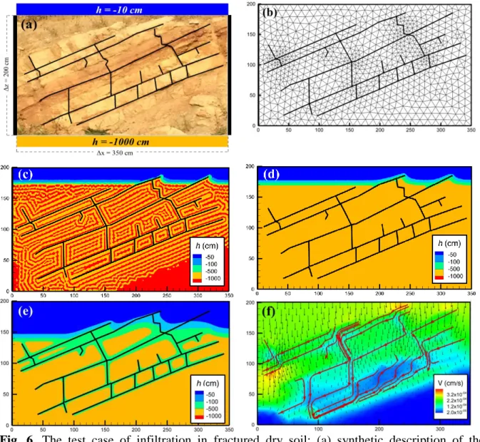
The geometry is inspired from a real fractured outcrop corresponding to a fractured aquifer in Jeita, Lebanon (Fig. 6a). Boundary conditions and soil parameters are similar to Huang et al (1996). Constant pressure heads of -10 cm and -1000 cm are imposed at the top and bottom boundaries of the domain, respectively, and an initial pressure head of -1000 cm representing a highly dry soil is assumed. Side boundaries are assumed impermeable. The hydraulic parameters of the porous matrix and fractures are given in Table 2. Fig. 6b shows the 1D/2D mesh gridding consisting of 1626 triangular elements for porous matrix and 272 linear elements for fractures. The duration of the simulation is set to be 3 × 105_{s (about 9 hours).}

The MH-Cons-1D/2D code is bound to run into convergence difficulties after 3 hours of simulation. A close look to the results at this time show that water front reaches the fractures (Fig. 6c). Spurious oscillations appear mostly near the fractures. Incoherent results can be observed with pressure head beyond physics (below -1000cm). These oscillations, causes the

convergence of the nonlinear solver to fail as the system of equations becomes ill-conditioned. The MH-Lump-1D/2D code runs without any convergence problems for the entire simulation duration. The results at t=3h are given in Fig. 6d. This figure shows stable solution free from spurious oscillations. With further advancement of time, fast preferential flow in the dry soil can be noticed along all the fracture elements (Fig. 6e). The demonstration of actual flow in the porous matrix and fractures can give better insights about the general direction of the flow and conductive behavior of the fractures (see Fig. 6f).

Fig. 6. The test case of infiltration in fractured dry soil: (a) synthetic description of the

problem: Geometry, fracture network and boundary conditions, (b) example of computational mesh, (c) pressure head map at t=3h with the MH-Cons-1D/2D code (without ML in fractures), (d) pressure head map at t=3h with the MH-Lump-1D/2D code (with ML in

fractures), (e) pressure head map at t=9h with the MH-Lump-1D/2D code and (f) corresponding simultaneous representation of the velocity field, velocity magnitude and the streamlines in fractures.

We also investigate the effect of the ML technique in fractures on the performance of the numerical models. Thus, we compare the CPU time of the MH-Lump-1D/2D and MH-Cons-1D/2D codes for different levels of mesh refinement. Fig. 7 gives the variation of the CPU for both codes versus the number of elements of the computational grids. It shows that the ML technique in fractures allows for a significant save in CPU time of 2 orders of magnitude whatever the level of mesh refinement. This gain in CPU time is mainly related to the better convergence properties of the new developed numerical scheme based on the ML technique in fractures.

Fig. 7. CPU time vs. number of elements of the computational mesh for both

MH-Lump-1D/2D and MH-Cons-MH-Lump-1D/2D codes.

5. Results: Field Scale Applications

This section aims at demonstrating the capacity of the proposed numerical scheme in simulating field cases at real scale. Thus, we use the new developed code (MH-Lump-1D/2D) to investigate the effect of climate change on groundwater resources in a karst aquifer/spring system in El Assal, Lebanon. In particularly, we use this code to evaluate the effect of fracture network on the hydrodynamic behavior of the aquifer and on the predictions of groundwater resources under potential impact of climate change. This application serves as showcase of the capacity of the developed numerical scheme not only to deal with large space scales, but also for large time scales as prediction of climate change effects are simulated for about 80 years, until 2099. It is also important to show the performance of the new scheme in simulating water table dynamic under highly variable recharge conditions.

El Assal karst spring is located at 1552 m (above sea level) in Mount Lebanon-Lebanon about 50 km from Beirut (Fig. 8a). Its catchment area of about 12 km2 is delineated based on tracer test experiments. The aquifer is composed of three zones of highly fissured, thinly layered basal dolostone overlain by dolomitic limestone, and limestone of Albian to Cenomanian age. The spring emerges at the top of underlying marls and volcanics of Aptian age. The catchment is characterized by a thick unsaturated zone (over 400 m). Dolines were mapped on the catchment to determine zones of point source infiltration. Disturbed representative soil samples were collected from different locations to determine the hydraulic properties such as particle size distribution and hydraulic conductivity at saturation. Fractures were mapped in the field along distinct sections. The recharge area is located between 1600 m and 2200 m elevation and is mostly dominated by snowmelt. The annual discharge of the spring ranges between 15-22 Mm3 based on high resolution monitoring since 2014 with maxima reaching 2 m3/s following snowmelt and minimum flow rates of 0.24m3/s during recession periods. The spring provides downstream villages in the Kesrouane district with about 24,000 m3 (0.28 m3/s) of water daily for domestic use and is an essential historic spring in the region. Further

information about the El Assal karst aquifer/spring system including the soil hydraulic parameters is discussed by Doummar et al. (2018). Fig. 8b shows the schematic profile of El Assal karst aquifer used as the domain of simulation. Calibration of the aquifer is out of the scope of this paper. The parameters of the porous matrix are used as in Doummar et al. (2018). According to that paper, the thickness of the fractures is assumed to be 1cm. The saturated hydraulic conductivity of the fractures was calculated using the cubic law and the other parameters were assumed to be similar to the one for the case of infiltration in dry soil (see Table 2).

Fig. 8. The representation of: (a) the location of the El Assal karst aquifer, (b) schematic

domain used to simulate the aquifer and (c) the monthly average recharge projection used for the simulations from 2013 to 2099. Time zero is June 1st, 2013.

5.2. Methodology for simulation and analysis

The domain is discretized using a triangular grid consisting of about 140K elements. No-flow boundary conditions are assumed at the right inland side and at the bottom surface representing the initial water table. At the left boundary, the spring is simulated by imposing nodal zero pressure head. The site is firstly simulated from 2013 to 2019 using real data (June 1st, 2013 to May 29th, 2019), in order to understand groundwater flow dynamic in the aquifer under 3 regimes of recharge including snowmelt, precipitation and dry periods. We then simulate the site with predicted precipitations for 2019-2099 (starting from June 1st, 2019) in order to evaluate future responses of the spring discharge variations caused by climate-change. We extract daily recharge time series (2019-2099) from Doummar et al. (2018),

where precipitation predictions are obtained from the IPSL_CM5 GCM (5th phase of the Coupled Model Intercomparison Project; Dufresne et al., 2013; Global Climatic Model) for Lebanon with a resolution of 0.25° based on the AgMERRA dataset (Ruane et al., 2015). In

Doummar et al. (2018) the scenario RCP 6.0 was adopted; meaning a stabilization of the radiative forcing value without overshoot pathway at 6 W/m2 after 2100. Projected raw data were corrected account for the elevation of the catchment area (1500-2200 m), using a constant lapse rate for T (-0.24 °C) and P (+5.5%) per 100 m elevation. For all simulations, we consider monthly averaged recharge variation. The results of simulations are analysed using the spatial maps of water content (θ) and three scalar metrics which are i) the dimensionless average saturation of the aquifer (𝑉_𝑚), ii) the maximum water table elevation (𝐻₀) and iii) the discharge rate at the spring outlet (𝑞_𝑜𝑢𝑡). The mathematical expression of the metrics is stated as following:

1

d

m e

V  _S 





(24)

(|Ω| is the area of the aquifer and Se is the element effective saturation defined in Table 1)

0 ( , , ) 0 ( ( , , )) h x y t H Max H x y t   ₍₂₅₎ 0 out _x

q

  

K H

_ (26)

5.3 Simulations with real data from 2013 to 2019

We simulate the aquifer using real data from June 1st, 2013 to May 29th 2019. Initially the domain is assumed to be at hydrostatic equilibrium. For this period, real recharge data are used for 2013-2016 and same data are imposed for 2016-2019, since data for 2016-2019 are not available. To investigate the effect of fractures on the groundwater dynamic we simulate the aquifer using 2 models. Both of them are developed using the code MH-Lump-1D/2D.

The first model considers the fracture network while the second one assumes the domain as homogenous (non-fractured). The corresponding maps of water content at the end of May 2019 are represented in Fig. 9. In general, similar profiles can be observed at the right side of the aquifer where fractures do not exist. A dry zone can be observed between two wet zones at the top and bottom. The appearance of this zone is due to the dry-wet cycle of recharge process. During a dry period, water saturation at the top aquifer decreases and then in a recharge period the upper surface is rapidly saturated. Still in the right part of the aquifer, but shifted left, where fractures occur, we observe that the fracture network do not have a dominant trend on the saturation distribution. Being highly permeable relative to the porous matrix, fractures tend to absorb and pass-through the flow faster than the adjacent porous matrix. This leads to high dry zones around the fractures which are easily noticed on the top of Fig. 9a. Around the centre of the aquifer, the preferential flow in the fractures, enhances water infiltration and expands horizontally the dry zone at the middle depth of the aquifer. At the left side, the fractures have more dominant effect as in contrast to the results of the no-fractured model; high saturation zone can be observed near the top surface.

(a)

(b)

Fig. 9. Maps of aquifer water content at the end of the simulation 2013-2019 (end of May

2019): (a) by considering the fracture network and (b) by neglecting the fractures

(a)

(b) (c)

Fig. 10. The flow streamline spatial distribution: (a) The general flow direction in the aquifer,

(b) General flow direction around fractures and (c) Flow around the stagnation points

The main groundwater flow in the aquifer (with fracture network) is presented in Fig.10 through streamlines. Vertical infiltration flow can be observed in the unsaturated zone. Near the water table the groundwater flow is horizontal towards the spring (Fig. 10a). Focusing in a more local point view point, it can be seen that flow generally tends to be absorbed and then travel through fractures (Fig. 10b). In certain cases, when a local maximum in the recharge distribution occurs and is followed by a relatively dry period, certain points appear near the fractured region which tend to absorb the water flow and create stagnant points nearby (Fig.

10c). This is mostly due to the fact that the water is drained faster in the fracture than in the porous matrix, resulting in higher conductivity (i.e. higher saturation) in the stagnant points compared to their adjacent points in the fracture.

Fig. 11 depicts the time variations of the scalar metrics (𝑉𝑚, 𝐻0, and 𝑞𝑜𝑢𝑡) using both the

fractured and non-fractured models. Fig. 11a confirms that there is a slight gap between both models regarding 𝑉_𝑚 but in general less amount of water is calculated with the fractured model. Referring to Fig. 11b, we can see that the level of water table is significantly affected by the fractures, which is coherent with the results discussed in Fig.9. Fig. 11c shows that the fractured model leads to higher water flux at spring outlet than the non-fracture model. These results indicate that the fracture networks enhance water infiltration in the aquifer. This increases the water discharge through the spring and decreases the amount of water stored in the unsaturated part of the aquifer. The results of Fig. 11c are coherent with the one in Fig. 11a. As in both models (fractured and non-fractured) the amount of influx from recharge is the same, the fact that more water is discharged with the fracture model (Fig. 11c) should lead to less retention of water in the aquifer with this model. This is completely true as Fig. 10a shows that less amount of stored water with the fractured model than the non-fractured one.

(a)

(b)

(c)

Fig. 11. Temporal distribution of (a) 𝑉_𝑚 (average amount of available water), (b) 𝐻₀

(maximum level of water table), and (c) 𝑞𝑜𝑢𝑡 (spring outlet discharge). Simulations from

2013 to 2019 (using real data) with both fractured (blue curves) and non-fractured (orange curves) models. Time zero represents 1st June, 2013.

In this section we investigate the effect of fractures on the predictions of water resources in the El Assal aquifer under climate change conditions. The main question in this context can be formulated as the following: “what is the effect of neglecting the fractures on the predicted results?” Thus, we simulate the aquifer with the predicted recharge from 2019 (June 1st 2019) to 2099. We started the simulation with hydrostatic equilibrium at June 1st 2013. We run the models from 2013 to end of May 2019 using real data (as in the previous section) and then for further time (since June 2019), we use the predicted recharge under climate change. The aquifer is simulated using 3 models. The first model, called F/NCC, considers the fracture network but neglects the effects of climate change on recharge. In this model, we assume that the recharge distribution of 2013-2019 occurs over the next eighty years, up to 2099. The second model, called F/CC, considers the fracture network and assumes variable recharge due to the effect of climate change (as in Fig. 8c). The last model neglects the fracture network (i.e. considers the domain as homogenous) and assumes variable recharge due to climate change. This model is denoted by NF/CC.

The results of the three models, regarding the map of water saturation, are presented in Fig. 12. At a first glance, and as expected, the water content and the saturated zone are higher in the model neglecting the variation of recharge due to climate change. When climate change effects are considered, the model including fractures (F/CC) leads to lower water table than the homogenous model (NF/CC). This understandable as the preferential flow in the fracture network enhances water infiltration through the unsaturated zone. Investigating further through the transient behavior of the proposed metrics, we can obtain better insights as in Fig.13. In this figure, it is clear that the effect of climate change will reduce the amount of available water in the aquifer as well as the water discharge at the spring outlet. This is clear from the differences between the model neglecting the climate change effects (red curves) and the models considering these effects (blue and orange curves). Under climate change

conditions, we can observe two regimes of time variation. Starting from hydrostatic equilibrium in 2020, during the first 40 years (from 2020 to 2060), the amount of water available in the aquifer, the water level table and the discharge flux at the spring will increase. After 2060, these metrics will exhibit a decreasing variation with time indicating less availability in water resources due to climate change. The general patterns of the results of the models F/CC and NF/CC indicates that neglecting fractures will lead to an overestimation of the available water resources in the aquifer. The difference in the estimated amount of available water with both F/CC and NF/CC models is clear from earlier time and persists during all the simulated period. The level of water table is slightly sensitive to fractures. Neglecting fractures in the model would lead to some periods where the level of water table is overestimated and other periods where it is underestimated. This is also the same for the water discharge at the spring.

(a)

(b)

(c)

Fig. 12. Spatial distribution of aquifer water content at year 2099: (a) F/CC model including

network and considering climate change effect on recharge and c) F/NCC model considering fracture network and ignoring climate change effect. Time zero is January 1st 2020.

(a)

(b)

(c)

Fig. 13. Temporal distribution of (a) 𝑉_𝑚, (b) 𝐻₀ , and (c) 𝑞_𝑜𝑢𝑡 for 2012-2099 period with the three models: F/CC (blue curves), NF/CC (orange curves) and F/NCC (red curves).

Considering the spring outlet discharge as the most important metric, we explore more the variability of this metric in Fig. 14. For the time period 0-7000 days (until 2033) it is clear that the discharge flux estimated with the fractured model is greater than the non-fractured model. Thus we focus the analysis in Fig. 14 on 2033-2099 span. This figure shows, simultaneously, the normalized distribution of the projected recharge along with the normalized difference between spring outlet discharge of the F/CC and NF/CC models (q_out). Both recharge and

out

q

 are normalized using the maximum value of the recharge influx. It is inferred from the figure that the higher variability in the recharge distribution results in higher variability of

out

q

 and higher inaccuracy in the prediction of the outlet discharge. The other interesting notation is the delay that is noticed for the response of the system at approximately 20000 days (= late-2060s). This point corresponds to the high recharge influx at 17000 days (= early-2060s). We suggest that this delay is due to the high fluctuation of the recharge at this period which will result in highly dry soil in the next dry season and saturated fractures. Saturated fractures (i.e. highly permeable fractures) tend to absorb the flow from the nearby matrix, resulting in much slower flow in the soil and consequently slower response of the spring. In other words, the fractures act as a magnet for the flow. This disturbs locally the general flow of the aquifer, resulting in a lag-time between the recharge event and the spring discharge response. This lag-time can grow over time due to the increase of variation of the recharge caused by the climate-change.

Fig. 14. Figure exploring the effect of fractures on the predicted spring outlet discharge under

climate change effect. q_out represents the normalized difference between the spring outlet discharge respectively estimated with the F/CC (considering fracture network) and NF/CC (ignoring fractures) models. Both recharge and q_out are normalized against the maximum value of the recharge influx.

6. Conclusion

Simulation of the VSF in discretely fractured domain is a computational challenge problem as it requires solving the RE in both porous matrix and dense fracture networks involving complicated geometry and high discontinuities in the hydraulic properties. Yet, solving RE in non-fractured domain is a challenging task that has been widely discussed in the literature. Existing numerical models of VSF in discretely fractured domains are limited to standard numerical techniques that hamper their applications in field studies. We develop a new