Development and testing of the AXBT Realtime Editing System (ARES)

(1)

Development and Testing of the AXBT Realtime

Editing System (ARES)

by

Lieutenant Junior Grade Casey R. Densmore,

United States Navy

B.S., United States Naval Academy (2018)

Submitted to the Department of Earth, Atmospheric

and Planetary Sciences

in partial fulfillment of the requirements for the degree of

Master of Science in Physical Oceanography

at the

MASSACHUSETTS INSTITUTE OF TECHNOLOGY

and the

WOODS HOLE OCEANOGRAPHIC INSTITUTION

September 2020

c

○2020 Casey R. Densmore.

All rights reserved.

The author hereby grants to MIT and WHOI permission to reproduce

and to distribute publicly paper and electronic copies of this thesis

document in whole or in part in any medium now known or hereafter

created.

Author . . . .

Department of Earth, Atmospheric and Planetary Sciences

August 13, 2020

Certified by . . . .

Steven R. Jayne

Senior Scientist

Woods Hole Oceanographic Institution

Thesis Supervisor

Accepted by . . . .

Glenn R. Flierl

Chairman, Joint Committee for Physical Oceanography

Massachusetts Institute of Technology

(2)

(3)

Development and Testing of the AXBT Realtime Editing

System (ARES)

by

Lieutenant Junior Grade Casey R. Densmore,

United States Navy

Submitted to the Department of Earth, Atmospheric and Planetary Sciences on August 13, 2020, in partial fulfillment of the

requirements for the degree of

Master of Science in Physical Oceanography

Abstract

Airborne eXpendable BathyThermographs (AXBTs) are air-launched, single use temperature-depth probes that telemeter temperature observations as a VHF-modulated frequency. This study describes the AXBT Realtime Editing System (ARES), which was developed to receive and quality control temperature-depth profiles with no exter-nal hardware other than a VHF radio receiver. The ARES Data Acquisition System performs fast Fourier transforms on windowed segments of demodulated signal trans-mitted from the AXBT and uses the resulting spectra to identify valid temperature-depth observations. When evaluated using 389 profiles, the ARES data acquisition system produced temperature-depth profiles nearly identical to those generated using a Sippican MK-21 processor, while reducing the amount of noise from VHF interfer-ence included in those profiles. The ARES Profile Editor applies a series of automated checks to identify and correct common profile discrepancies, before displaying the pro-file on an editing interface that provides simple user controls to make additional cor-rections. When evaluated against 1,177 tropical Atlantic and Pacific AXBT profiles, the ARES automated quality control system successfully corrected 87% of the profiles without any manual intervention necessary. The ARES Data Acquisition and Pro-file Editing Systems performed exceptionally well when operationally tested with 44 AXBTs during Hurricane Dorian (2019), enabling high resolution observations across key oceanic features including Dorian’s cold wake and the Gulf Stream. Necessary future work includes improvements on the automated quality control algorithm and evaluation against a more diverse dataset of temperature-depth profiles.

Thesis Supervisor: Steven R. Jayne Title: Senior Scientist

(4)

(5)

Acknowledgments

This research was funded by the U.S. Navy’s Civilian Institution (CIVINS) Office with the MIT-WHOI Joint Program. Additionally, this work was funded by the Office of Naval Research, grant number N000141812819. I would not have reached this point without the influence of many people, and while I cannot list them all here within a reasonable word count, I am truly appreciative of their guidance and support.

First, I am thankful for my mom and grandparents, who encouraged my fascina-tion with severe weather from a young age and supported me uncondifascina-tionally along the way. You may have gotten more than you bargained for with the tornado chas-ing and hurricane huntchas-ing, but your encouragement enabled my interest to become a passion.

Second, I am grateful to the USNA Oceanography Department faculty who pro-vided me with the tools necessary to succeed in the Joint Program. I would like to particularly thank my undergraduate research advisers CAPT Elizabeth Sanabia and Dr. Brad Barrett, who guided me through my first experiences researching and publishing peer-reviewed science.

CAPT Sanabia also brought me into TROPIC, which introduced me to one of the most amazing experiences in my life: flying with the Hurricane Hunters. I am grateful to CAPT Sanabia for her continued professional and academic mentorship over the past few years. I also want to thank the members of the 53rd Weather Reconnaissance Squadron for their support and patience over those years as we launched hundreds of AXBTs on training and storm missions.

Over TROPIC I met and worked with a lot of amazing people. I want to par-ticularly thank Jordan, Grace, Shannon and Jake for the countless hours they spent testing various versions of ARES. Additionally, this work would not have been possi-ble without technical guidance from Matt Kuhn, Jeff Kerling, and Kyle Rushing from the Naval Oceanographic Office.

Also during TROPIC I met Steve Jayne, who became my advisor for the MIT-WHOI Joint Program. Steve’s guidance enabled me to select classes and research topics to take full advantage of the opportunities available to me in the Joint Program. Steve is one of the smartest people I have ever met, and I aspire to one day be a scientist of his caliber. I am also grateful to the professors and administrators in the Joint Program, as well as my classmates whom I met along the way. I would particularly like to thank Stephan Gallagher and Jeff Grabon, two exemplary Naval officers and even better friends who were willing to mentor a clueless Ensign starting his Naval career in an unconventional way.

Finally, I am eternally grateful to my wife for her constant love and support throughout my time in Massachusetts. Hannah, I love you more than I can put into words and I am so lucky to get to spend the rest of my life with you.

(6)

(7)

List of Figures

1-1 (a) AXBT deployment locations and (b) tracks of tropical cyclones in which AXBTs were deployed for TROPIC between 2011 and 2019. Figures from [1]. . . 20 2-1 (Left) components of an AXBT (from left to right: storage canister,

AXBT casing, surface float, and thermistor probe) and (right) a typi-cal AXBT deployment diagram. Figure from www.hurricanescience.

org/science/observation/aircraftrecon/expendableairborneinstruments/ (images originally provided by the USCG International Ice Patrol). . 25 2-2 A Hurricane Hunter loads an AXBT into its launch tube. . . 26 2-3 Residual temperature differences between the standard Navy and

MK-21 conversion equations (black lines), a best fit equation for those resid-uals (red line), and the documented Sippican conversion equation (Eq. 2.5; green line). . . 31 3-1 The ARES Data Acquisition System graphical user interface. . . 34 3-2 The ARES Data Acquisition System settings window. . . 37 3-3 The ARES temperature/depth conversion equation settings window. . 39 3-4 The ARES GPS configuration settings window. . . 40 3-5 A WiNRADIO G39WSBE software-defined receiver (image from www.

winradio.com/home/g39wsbe.htm). Ports on the front-left face of the receiver are: (top left) analog audio out (SMA), (top right) VHF in (SMA), (bottom left) power (2.5 mm), and (bottom right) digital audio out (serial). . . 41

(12)

3-6 The WiNRADIO receiver array used in this study. . . 42 3-7 Process to demodulate a received AXBT VHF signal and generate the

encoded temperature-depth profile. . . 43 3-8 Diagram of nested functions in the ARES Data Acquisition System

thread class, with functions listed on arrows using PyQt signals (arrows out of the Data Acquisition System thread block) and slots (arrows into the thread block) to pass information to and from the ARES user interface. . . 46 3-9 Sequence to pull and process segments of PCM data to identify valid

temperature-depth measurements transmitted from an AXBT. . . 47 3-10 (a) Distribution of maximum signal levels (dB) for the 531 reprocessed

profiles. The vertical gray line denotes the required minimum peak signal level for all profiles analyzed (𝑆𝑃𝑀 𝐴𝑋 = 75 dB). (b,c)

Distri-butions of (b) signal levels (dB) and (c) signal-to-noise ratios for all observations in the 459 profiles whose maximum signal level exceeds the threshold in (a). Vertical lines represent minimum signal level and ratio thresholds (solid and dashed lines correspond to minimum and trigger thresholds, respectively) applied when evaluating Data Acqui-sition System performance. . . 54 3-11 Distributions of observations for all observation times versus (a) signal

levels and (b) signal-to-noise ratios. Profiles were standardized so zero seconds (vertical lines) denotes the first observation that satisfied the minimum triggering thresholds. Triggering and general thresholds are denoted by horizontal dashed and solid lines, respectively. . . 55 3-12 Comparison of 2m bin-averaged temperatures processed by the MK-21

and by ARES. Yellow lines denote a 1:1 relationship and magenta lines represent best fits for the data. . . 56

(13)

3-13 Average 10m standard deviations for temperature-depth profiles pro-cessed by the MK-21 and by ARES (shading denotes one standard de-viation from the mean dede-viations). The solid black line denotes rated temperature accuracy for Sippican AXBTs [2]. . . 57

4-1 The ARES profile editing graphical user interface. . . 62 4-2 The ARES Profile Editor ASCII file selection interface. . . 64 4-3 File formats for (a) FIN/NVO and (b) JJVV files. Note that the FIN

file used in (a) is truncated below 48m, but the same temperature-depth format is continued for the remainder of the file. . . 67 4-4 The ARES profile editor settings window. . . 69 4-5 Data flow through the VHF interference correction component of the

autoQC algorithm. . . 71 4-6 Distributions of (a) autoQC algorithm performance, (b) operator

cor-rections for profiles that required manual edits, and (c) quality control codes for bad profiles. Note that (b) and (c) show the distributions of profiles from the dark green and red wedges (respectively) in (a). . . . 75 4-7 Root mean square temperature differences (𝑜_{C, solid red line) for}

ARES-and SASEA-processed profiles. Shading denotes mean temperature dif-ferences plus and minus one standard deviation. The solid black line denotes rated temperature accuracy for Sippican AXBTs [2]. . . 76 4-8 Examples of profiles that required manual edits, for: (a) missed bottom

strike, (b) false positive bottom strike, (c) excessive interference at depth, (d) erroneous mixed layer feature, (e) temperature spike, and (f) missed profile false start. Unedited (raw) profiles are plotted as grey lines, and incorrectly (autoQC) and correctly (manually) quality-controlled profiles are overlaid in red and green, respectively. . . 77

(14)

5-1 Hurricane Dorian (2019) track and intensity, environmental sea surface temperatures on 30AUG, and deployment locations (by mission) for AXBTs processed with ARES in realtime. Inset satellite imagery show storm-relative float deployment locations for each mission. . . 82 5-2 (a) Distribution of maximum signal levels (dB) for Hurricane Dorian.

The vertical gray line denotes the required maximum peak signal level for all profiles analyzed (𝑆𝑃𝑀 𝐴𝑋 = 65𝑑𝐵). (b and c) Distributions of

(b) all signal levels (dB) and (c) all signal-to-noise ratios (%) for all observations in Hurricane Dorian. Vertical lines represent minimum signal level and ratio thresholds (solid and dashed lines correspond to general and trigger thresholds, respectively) applied when evaluating data acquisition system performance. . . 83 5-3 Distributions of observations in Hurricane Dorian for all observation

times versus (a) signal levels and (b) signal ratios. Profiles were stan-dardized so zero seconds (vertical lines) denotes the first observation that satisfied the minimum triggering thresholds. Triggering and gen-eral thresholds are denoted by horizontal dashed and solid lines, re-spectively. . . 84 5-4 Mean 10-m standard deviations (solid line) and ± one standard

de-viation of the 10-m standard dede-viations (shading) for the 43 AXBT profiles received with WiNRADIO receivers during Hurricane Dorian, processed with the signal level and ratio thresholds shown in Figs. 5-2 and 5-3. . . 85 5-5 AXBT profiles collected with ARES in Hurricane Dorian, organized by

mission. . . 86 5-6 (a) Temperature-depth profiles and (b) signal level (𝑆𝑃; Eq. 3.3) versus

time for (dashed lines) possible late starts and (solid lines) adjacent profiles. . . 87

(15)

5-7 Cross-track transects of AXBT observations for Hurricane Dorian col-lected at (left) 01SEP2019 0000 UTC, 73𝑜_{W and (right) 02SEP2019} 0000 UTC, 76𝑜W. Dashed black lines mark AXBT observation loca-tions and magenta lines denote Hurricane Dorian’s center latitude on crossing each transect. . . 89 5-8 Cross-Gulf Stream transects (approximately 28.3𝑜_{N, 80.2}𝑜_{W to 27.6}𝑜_N,

78.8𝑜W) of AXBT observations for Hurricane Dorian collected at (left) 02SEP2019 0000 UTC and (right) 03SEP2019 1200 UTC. Dashed black lines mark AXBT observation locations for each transect. . . 90 5-9 Storm-relative (distances in km) anomalies of SST, TCHP, and D26𝑜_𝐶. 91

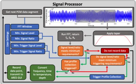
6-1 Comprehensive data flow for the AXBT Realtime Editor System, in-cluding both the Data Acquisition System (top) and Profile Editing System (bottom) separated by a horizontal dashed line. . . 94

(16)

(17)

List of Tables

3.1 WiNRADIO application-programming interface functions integrated in the ARES Data Acquisition System. . . 44 3.2 Audio file processing time means and standard deviations, and

corre-sponding temperature resolution, for several combinations of FFT win-dows and taper use. Processing time means and standard deviations (comma-separated) are expressed as the ratio for a given processing time to the corresponding time for the same file using no taper and a window of 0.3 seconds. . . 59 4.1 ARES quality control codes for post-processed AXBT

temperature-depth profiles. . . 67 5.1 AXBT profile breakdown by quality control codes. Quantities in

paren-theses include AXBTs that were not collected with ARES but are not included in the totals. . . 85

(18)

(19)

Chapter 1 Introduction

1.1 Motivation

Obtaining in-situ temperature-depth profiles remains a necessity for observational oceanography. While significant advances in satellite capabilities have enabled global sea surface temperature observation, resolving subsurface features (e.g. mixed layer depth and ocean heat content) and observing conditions under extremely cloudy skies require in situ measurements [3]. The eXpendable BathyThermograph (XBT) is a commonly-used sensor capable of collecting a single temperature-depth profile, typ-ically to several hundred meters depth. The aircraft-launched variant, the Airborne eXpendable BathyThermograph (AXBT), enables aircraft to measure upper-ocean temperatures in remote or inhospitable regions that are difficult to access by ship.

Applications for AXBTs range from scientific (e.g. observations of multi-scale pro-cesses, particularly in remote or inhospitable conditions) to military (e.g. underwater acoustics). One recent example of scientific use of AXBTs, which served as the mo-tivation for this thesis, is the Training and Research in Oceanic and atmospheric Processes In Cyclones (TROPIC) field campaign [4], which has run from 2011-2020. TROPIC is conducted to make sustained observations of upper-ocean temperatures beneath tropical cyclones. ARES was developed in coordination with TROPIC as a data acquisition and quality control solution to replace the existing systems.

(20)

1.2 TROPIC Program Background

From 2011 through 2019, members of the TROPIC program deployed 1,524 AXBTs on nearly 200 flights, including missions through 30 named tropical cyclones in the At-lantic and eastern/central Pacific basins. These AXBTs were launched from WC-130J aircraft on a not-to-interfere basis during training and reconnaissance missions by the US Air Force 53rd Weather Reconnaissance Squadron (Hurricane Hunters). Success-ful AXBT profiles were quality controlled and transmitted to the Global Telecommu-nications System (GTS) for integration into numerical weather prediction models.

Figure 1-1: (a) AXBT deployment locations and (b) tracks of tropical cyclones in which AXBTs were deployed for TROPIC between 2011 and 2019. Figures from [1].

Through 2019, TROPIC participants collected AXBT data onboard the aircraft with a Mobile Ocean Observing System (MOOS; [4]) designed and built by the Naval Research Laboratory (NRL), Monterey, CA. This system includes a power converter, MK-10A Receiver, two Marantz audio recorders, MK-21 Data Acquisition System, and a processing computer, all encased within two approximately 2’x2’x3’ boxes to-gether weighing over 200 lbs. Signals received via the aircraft’s VHF antenna are

(21)

de-modulated by the MK-10A Receiver before being simultaneously passed to a Marantz audio recorder and the MK-21 Data Acquisition System. The MK-21 calculates tem-perature and depth observations from the incoming audio stream and sends those observations to the processing computer, where they are simultaneously logged and plotted on the MK-21 software’s user interface.

After an AXBT profile has been fully recorded, it is quality controlled using the System for At-Sea Environmental Analysis (SASEA), a software package operated in a MATLAB environment. During this quality control process, raw temperature-depth profiles are despiked and smoothed before inflection points are automatically detected for recording. Users then manually select additional points to ensure a sufficient vertical resolution to pass quality control systems for numerical models (e.g. every 10 m in the upper 100 m). These quality controlled profiles are then saved as both 1 m resolution text files and JJVV (BATHY) files, the latter of which are transmitted to the GTS. Additional information about the data acquisition and quality control processes for TROPIC can be found in [4].

While effective, this system has several disadvantages. First, the MOOS system is both large and heavy, making it difficult to carry on and off of the aircraft. Ad-ditionally, the system includes a large number of interconnected components with cables that must be attached and removed every time the system is setup and stored, introducing the possibility for user error or loose and/or degraded connectors that prevent AXBT signals from being properly received. Moreover, the quality control process requires both manual input of profile metadata (e.g. drop time and position) and manual profile editing, introducing the potential for operator error. This quality control system is also somewhat time-intensive (requiring approximately 10 minutes per profile for a well-trained operator), increasing the margin for error during rapid or extensive AXBT deployments. Finally, a major objective of TROPIC is to transition AXBT observation capabilities to the Hurricane Hunters. This places an additional emphasis on reducing requisite space (for integration into onboard systems) and time (due to the fast-paced work tempo for aircrew in the storm environment) constraints of the system, as well as the degree of training required for operators.

(22)

1.3 Contribution and Organization

The AXBT Realtime Editing System (ARES) was developed to accomplish several objectives:

1. Incorporate most hardware-defined features from MOOS as software-defined functions to reduce the amount of necessary hardware

2. Enable simultaneous processing of multiple AXBTs on different VHF channels 3. Integrate system date/time inputs and a connected GPS receiver to auto-populate

fields on AXBT launch and minimize errors due to incorrectly entered drop in-formation

4. Combine data acquisition and profile editing into a program with a single graph-ical user interface so users can seamlessly transition from data receipt to quality control

5. Minimize requisite oceanographic background knowledge on the part of users receiving and quality controlling AXBT-measured profiles

ARES is composed of two integrated subsystems: the Data Acquisition System, which demodulates and Fourier transforms received VHF signals and calculates the corresponding temperature depth profile, and the Profile Editing System, which ap-plies automatic quality control checks to correct for common issues and presents the resulting profile to the user to apply any additional corrections before saving. This thesis and the accompanying research provide the following contributions:

∙ Developing the software-hardware suite for the AXBT Realtime Editing System (ARES)

∙ Describing the functionality of ARES

∙ Providing instructions to install and operate ARES, as well as to troubleshoot possible issues

(23)

∙ Evaluating the performance of the ARES Data Acquisition and Profile Editing Systems against the existing TROPIC dataset

∙ Examining the performance of ARES in an operational setting during aerial weather reconnaissance missions through Hurricane Dorian (2019)

∙ Presenting a case study of useful results from AXBT profiles collected and quality-controlled with ARES in Hurricane Dorian

The remainder of this thesis is organized as follows. Chapter 2 provides more detailed background about Airborne eXpendable BathyThermographs (AXBTs) and requirements for AXBT data acquisition and post-processing systems. Chapter 3 de-scribes and evaluates the performance of the ARES Data Acquisition System. Chap-ter 4 describes and evaluates the performance of the ARES Profile Editing System. Chapter 5 examines the performance of ARES during Hurricane Hunter operations in Hurricane Dorian (2019) and presents some of the results enabled by collection of AXBT data at high spatial resolution with ARES. Chapter 6 includes a summary of ARES functionality and avenues for future work. Finally, the appendices include (A) installation and (B) troubleshooting guides and (C) additional technical details about ARES source code and compilation.

(24)

(25)

Chapter 2 Background

2.1 AXBT System Overview

The Airborne eXpendable BathyThermograph (AXBT) is an air-launched, single use temperature depth probe capable of observing ocean temperatures in the upper 400 to 900 m (depending on the AXBT variant used). Components of an AXBT are shown in Fig. 2-1, left panel.

Figure 2-1: (Left) components of an AXBT (from left to right: storage canister, AXBT casing, surface float, and thermistor probe) and (right) a typical AXBT

deploy-ment diagram. Figure from www.hurricanescience.org/science/observation/

aircraftrecon/expendableairborneinstruments/ (images originally provided by the USCG International Ice Patrol).

(26)

The leftmost item in Fig. 2-1 is a plastic canister commonly used to store AXBTs. Launch methods vary depending on launching platform, but in many cases (including for deployments associated with this thesis) the AXBT (gray cylinder second from the left in Fig. 2-1, left panel) is removed from the canister and placed in an A-sized (approximately 13 cm in diameter) launch tube (Fig. 2-2). This tube is connected to the airframe and has a mechanism (e.g. a lever) to briefly open a seal in the base of the tube, allowing the pressure difference between the aircraft interior and surrounding environment to push the AXBT out of the tube. The AXBT then descends towards the surface beneath a small parachute; descent times can range between 120 and 150 seconds for a launch from 10,000 feet, depending on atmospheric conditions.

Figure 2-2: A Hurricane Hunter loads an AXBT into its launch tube.

Upon reaching the surface, the entire AXBT submerges (Fig. 2-1, right panel) and deploys a surface float (small red object second from the right in Fig. 2-1, left panel) that separates from the parachute and plastic casing (which self-scuttles). The surface float inflates a small bag to maintain positive buoyancy, and a saltwater-activated battery triggers the float to begin transmitting an unmodulated VHF carrier frequency from its antenna. This carrier frequency is one of 99 standard sonobuoy VHF frequencies between 136 and 173.5 MHz, and is either selected by the operator prior to launch or built into the AXBTs hardware (depending on the AXBT model). Simultaneously, water-soluble adhesive retaining a thermistor probe (rightmost object in Fig. 2-1, left panel) in the base of the surface float dissolves, releasing the thermistor to descend through the water column. The thermistor remains connected to the

(27)

surface float via a very thin copper wire through which it transmits temperature observations. The maximum observation depth of an AXBT is limited by the length of this wire; after the thermistor exceeds this rated depth, the wire breaks, the AXBT stops transmitting, and the surface float self-scuttles [5, 6].

As the probe descends, ambient ocean temperature alters the resistivity (and therefore resistance) of an integrated thermistor element. The thermistor’s resistance in turn modifies the voltage of the integrated circuit, which is the input to a voltage-controlled oscillator (VCO) in the probe. The VCO outputs an alternating current whose frequency is proportional to the input voltage (and thus thermistor resistivity and ocean temperature). This alternating current travels up the wire to the surface float, and it is the audio-range frequency of this alternating current that is frequency modulated (FM) into the VHF carrier frequency and transmitted to the observing aircraft for data acquisition and processing. Recovering a temperature-depth profile from this signal requires empirical frequency-to-temperature and fall rate equations, discussed in the following section.

2.2 AXBT Processing

2.2.1 Data Acquisition

Processing signal from an AXBT and returning a temperature-depth profile from signal received through a VHF antenna involves repeating the following steps several times per second for the duration of AXBT profile transmission:

1. Demodulating a segment of FM VHF signal to recover the original AXBT signal (including a temperature-encoded audio-range frequency)

2. Applying a signal processing technique (e.g. Fourier transform) to recover the peak frequency from that AXBT signal segment

3. Applying empirical frequency-to-temperature and fall rate equations to deter-mine the corresponding temperature-depth point for that signal segment

(28)

Demodulating incoming VHF FM signal and outputting a PCM audio stream requires a radio receiver, which may fall into one of two categories: hardware- or software-defined. Hardware-defined receivers demodulate signals from one or more fixed frequencies, and generally have physical control inputs (e.g. knobs, switches) to control settings such as demodulated signal volume. For example, the Mobile Ocean Observing System (MOOS), used during TROPIC from 2011-2019, integrates a hardware-defined MK-10A Receiver capable of demodulating FM signals from VHF channels 12, 14, and 16 (170.5, 172.0, and 173.5 MHz, respectively).

Software-defined receivers function similarly to their hardware-defined counter-parts, but are controlled by a connected computer which also often handles much of the signal processing tasks required for demodulation. These receivers require an application programming interface (API) through which the computer communicates with the receiver. Though requiring an operating computer may be considered a disadvantage, software-defined receivers provide multiple advantages over hardware-defined receivers. First, they enable seamless integration of the receiver with other relevant computer software (in this context, controlling whether a selected receiver is actively demodulating, as well as its target VHF channel/frequency, from within an AXBT data acquisition program). Additionally, software-defined receivers typically require less analog hardware, potentially mitigating spatial and financial limitations. Given these advantages, ARES was developed with integrated support for the WiN-RADIO W39GSBE software-defined receiver (discussed further in Chapter 3).

Regardless of demodulation method, windowed segments of the output audio stream from the receiver must be processed to identify peak frequencies at dis-crete times and subsequently determine the corresponding observed temperatures and depths. The current industry standard for this task is the Sippican MK-21 Data Acquisition System. This processor and its accompanying software are designed to process received (and for airborne variants, demodulated) signals from a range of ship-and air-launched expendable ocean probes. Processed profiles are transferred to the operating computer in realtime and saved for further quality control and use. In many data acquisition systems, audio streams may also be directed to an audio recorder so

(29)

profile recordings can be reprocessed to correct for errors. It should be noted that other AXBT data acquisition systems exist, such as the Ocean Data Acquisition and Analysis Recorder (ODAAR; [7]).

Although these tasks typically require external hardware in existing AXBT data acquisition systems, both the signal processing and audio recording can be accom-plished entirely on the processing computer. This enables the development of a system with significantly less required hardware (advantageous due to weight, space, and cost constraints) but which also increases the burden on the processing computer. ARES was developed so these tasks are software-defined, and their data flow and computa-tional expense are both examined in Chapter 3.

2.2.2 Empirical Conversion Equations

Temperature and depth conversion equations are the source of a range of literature aiming to identify uncertainty and correct for a host of error sources such as internal noise and thermal lag (e.g. [2, 5, 6, 8, 9, 10, 11]). The standard Navy fall rate equation to determine observation depth from elapsed time since the first signal was identified, based on presumed fall rate of the probe (1.52 m/s) is simply 𝑧 = 1.52∆𝑡. The corresponding conversion relating temperature (𝑜C) and frequency (Hz) originally specified by Naval Air Systems Command (NAVAIR) to AXBT manufacturers is a simple linear equation (Eq. 2.1; [6]; personal communication, J. Kerling, 2020).

𝑓 = 1440 + 36𝑇 𝑇 = −40 + (2.778 × 10−2)𝑓

(2.1)

Several studies have sought to identify more accurate, higher order frequency-to-temperature conversion equations. For example, [12] tested frequency-to-temperature calibrations for 48 Sippican AXBTs and identified a cubic conversion equation:

(30)

Additionally, Sippican released a fifth-order conversion [5]:

𝑇 = − 126.662 + (0.219954)𝑓 − (1.70509 × 10−4)𝑓2+ (7.70543 × 10−8)𝑓3 − (1.7958 × 10−11)𝑓4 + (1.73823 × 10−15)𝑓5

(2.3)

However, [6] determined that Eq. (2.2) underestimated temperatures by approxi-mately 0.1𝑜_{C and Eq. (2.3) overestimated them by approximately 0.2 - 0.5}𝑜_{C, and} proposed and tested a linear equation demonstrated to be more accurate:

𝑇 = −38.6045 + (2.71075 × 10−2)𝑓 (2.4)

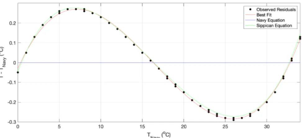
A more recent, similar but not identical fifth-order Sippican conversion (Eq. 2.5) also exists (personal communication, J. Kerling, 2020). The use of this (or an ex-tremely similar) updated Sippican conversion equation in the MK-21 Data Acquisition System was verified by examining MK-21 output for known frequency inputs using a BANDIT Box. The BANDIT Box is useful for testing sonobuoy data acquisi-tion systems by outputting a VHF modulated test signal (for AXBTs, this signal is a single frequency following the standard Navy conversion, Eq. 2.1). Because the VHF-modulated frequencies generated and output by the BANDIT box are known, observed residuals (Fig. 2-3, black lines) between temperatures input to the MK-21 Data Acquisition System and those output from the MK-21 following the propri-etary equation were used to identify a best fit estimate (Fig. 2-3, red line), which is compared to the updated Sippican conversion (Eq. 2.5; Fig. 2-3, green line). The root-mean-square difference between the residual best fit and modified Sippican equation are less than 0.02𝑜_{C, well within the threshold for AXBT instrumental error.}

𝑇 = − 126.662 + (0.219954)𝑓 − (1.70596 × 10−4)𝑓2+ (7.705434 × 10−8)𝑓3 − (1.79581 × 10−11)𝑓4+ (1.73823 × 10−15)𝑓5

(31)

Figure 2-3: Residual temperature differences between the standard Navy and MK-21 conversion equations (black lines), a best fit equation for those residuals (red line), and the documented Sippican conversion equation (Eq. 2.5; green line).

Similar analyses exist for AXBT probe fall rate equations. As with frequency conversions, Sippican released a higher order depth equation (Eq. 2.6; [5]).

𝑧 = 1.5926∆𝑡 − 0.00018∆𝑡2 (2.6)

However, [6] identified a depth equation that the author found to be more accurate for both shallow and deep AXBTs:

𝑧 = 1.6325∆𝑡 + (1.5553 × 10−5)∆𝑡2 (2.7)

It is worth noting that the conversion equations listed here are far from comprehensive, but are simply provided as examples of the range of equations tested and employed over the past several decades. For a more thorough discussion, see [11].

2.2.3 AXBT Profile Quality Control

After the AXBT has finished transmitting, the received profile must be qual-ity controlled to correct for noise, interference, and AXBT measurement errors. In TROPIC, this was previously accomplished with the System for At-Sea Environmen-tal Analysis (SASEA; [13]). SASEA provides an interface for analysis and quality control from a range of ship- and air-launched probes. Options for XBT and AXBT

(32)

profile quality control include profile smoothing, surface correction, and individual point addition and removal. Although fully automated processing systems are known to exist, these systems are not documented in published literature (S. Paul, NOAA AOC, 2020, personal communication).

Various organizations have developed guidelines for XBT/AXBT quality control routines. For example, NOAA’s Atlantic Oceanographic and Meteorological Labora-tory (AOML) references a quality control cookbook for XBTs developed by Australia’s Commonwealth Scientific and Industrial Research Organisation (CSIRO) XBT pro-gram [14]. This document includes guidelines for common ocean thermal structures and seasonal variability, quality control procedures to identify common profile dis-crepancies, and quality control flags to summarize those discrepancies. A similar (though much older) manual published by the Naval Oceanographic Office provided guidance for XBT quality control for the US Navy [15].

These quality control guidelines and routines all detail basic requisite background oceanographic knowledge, including an understanding of typical thermal structures for the region and season in which the XBT/AXBT was launched. Additionally, these routines detail common discrepancies and failure modes, as well as a series of quality control flags used to categorize the quality of any XBT/AXBT profile. Together, these highlight the potential for an advanced XBT/AXBT quality control interface. Such an interface could automatically apply checks and corrections for common profile failure modes, provide an interface for users to verify profile accuracy and apply additional edits if necessary, integrate global climatology and bathymetry data to guide both automated and user-driven profile quality control, and include inputs for users to select from a range of quality control flags to categorize profile accuracy in a standardized manner.

(33)

Chapter 3 ARES Data Acquisition System

The AXBT Realtime Editing System (ARES) Data Acquisition System is designed to receive digital pulse code modulated (PCM) audio data containing an AXBT signal and produce a viable temperature-depth profile from that data. ARES is compatible with WiNRADIO software-defined radio receivers, which demodulate a VHF signal transmitted from an AXBT and exporting the resulting PCM data to ARES for pro-cessing. Additionally, previously recorded WAV files can be imported into ARES to generate a temperature-depth profile. ARES integrates the signal processing ca-pabilities of the MK-21 or similar hardware and audio recorders as software-defined functions, reducing the equipment necessary to launch and process data from AXBTs. The remainder of this chapter is organized into three sections: Section 3.1 describes the ARES Data Acquisition System interface, Section 3.2 discusses necessary hard-ware setup, data flow, signal processing details, and additional features of the Data Acquisition System, and Section 3.3 evaluates the capabilities of the Data Acquisition System using raw (PCM) audio data from profiles launched during the TROPIC field program from 2011-2019.

(34)

3.1 Data Acquisition System Interface Description

3.1.1 Layout

An ARES Data Acquisition System graphical user interface (GUI) tab is opened by default when starting ARES. Additional Data Acquisition System tabs can be opened by either selection Options > New Data Acquisition System Tab or using the keybinding ctrl+N. The Data Acquisition System window is divided into three sections (Fig. 3-1):

1. Raw, realtime temperature-depth profile plot (left)

2. Tabular temperature-depth profile and signal information (lower right) 3. Datasource, VHF, and profile metadata configurations (upper right)

Figure 3-1: The ARES Data Acquisition System graphical user interface.

The upper-right corner of the GUI provides options for the user to control the Data Acquisition System, and includes two columns with user inputs. At the top of the left column, a dropdown menu allows the user to select the data source from which AXBT data is being processed. The datasource selection dropdown menu

(35)

automatically has two default options: "Test", which processes a test signal (from a raw audio file distributed with ARES), or "Audio", which prompts the user to select a raw WAV file to be reprocessed. Additionally, on Windows systems with the WiNRADIO drivers installed, any connected WiNRADIO receivers will be listed by serial number in order to process data in realtime. Because each receiver can only demodulate one channel at a time, ARES prevents the user (with an accompanying warning message) from selecting the serial number for a WiNRADIO that is actively receiving in a different tab.

If a connected WiNRADIO receiver is selected, the two spinboxes immediately be-low the datasource selection menu (labelled "VHF Channel" and "VHF Frequency") allow the user to select the VHF frequency that the receiver demodulates, either directly by frequencies or by selecting the corresponding sonobuoy VHF channel (se-lecting a new frequency will update the selected channel, and vice versa). The VHF channel and frequency being demodulated can be changed while a receiver is actively processing data.

Buttons for the user to start and stop data acquisition are located at the bottom of the left column. Data acquisition should be started when the profile is launched, to ensure that the recorded date, time, and (as applicable) position are representative of the moment the AXBT was launched. Data acquisition can be restarted after being stopped (except when reprocessing from audio files), and the time elapsed will be preserved from the initial start selection. However, for realtime processing, any data received while the Data Acquisition System was stopped is lost. After processing has been initiated (by selecting start), the user cannot switch between Test/Audio/Receiver data sources. The selected receiver can be changed if multiple receivers are connected, but to do this the user must stop processing, select a different receiver, and then resume processing.

While actively processing, the table in the lower-left section of the screen is up-dated in realtime with incoming data from an AXBT. The table’s columns are (from right to length): time (seconds), frequency (Hz), signal level (dB), signal ratio (%), depth (meters) and temperature (𝑜C). The time and frequency fields list the time

(36)

elapsed since "Start" was selected and the peak frequency of the signal currently be-ing received. If a signal’s peak frequency is in the expected range correspondbe-ing to realistic temperature values (defined by user settings, default 1300-2800 Hz) and the observed signal level and signal-to-noise ratio (SNR; these values are displayed in the 𝑆𝑃 and 𝑅𝑃 columns in the table, respectively and described in more detail in Section 3.2.2) meet the required minimum thresholds (which are defined in the user settings as described in the next section), then the temperature and depth are calculated and appended to the profile plot, and the corresponding row in the table will appear green. If the minimum signal level and SNR thresholds are not met, temperature and depth are not calculated or appended to the profile plot, and the corresponding row in the table will appear gray.

The right column of text provides inputs to record AXBT drop information: date, time, latitude, longitude, and platform identifier (e.g. aircraft tail number). For realtime drops (when the selected datasource is a WiNRADIO serial number), the date, time will be autopopulated from the system date and time, and the position will be populated from a connected GPS receiver (if configured in ARES preferences, as discussed in the following section). This autopopulation option is configurable in the ARES settings. After processing AXBT data and entering the corresponding drop information, selecting "Process Profile" will first prompt the user to save the raw profile data (this is configurable in ARES settings) before loading the raw profile into a Profile Editor tab (discussed in Chapter 4).

3.1.2 Settings

Data Acquisition System Settings

The Data Acquisition System settings are divided into four sections: autopopu-lation options, file save formats, Data Acquisition System thresholds and windows, and additional settings. The autopopulation options (top left) control whether ARES automatically updates the recorded drop information (in the right column in the Data Acquisition System tab) whenever "Start" is selected for the first time in a tab.

(37)

Au-topopulation is not used when data is being reprocessed from a raw audio file (when "Audio" is the selected data source). Four file save formats (discussed in Section 3.2.3) are also selectable. Below these options are three additional user settings that control user prompts that appear when attempting to save the raw data and transition to a Profile Editor mode.

Figure 3-2: The ARES Data Acquisition System settings window.

The rightmost column of settings control the windows and thresholds used to process AXBT data. The "FFT Window" is the length of each window of data (in seconds) used to determine peak frequency and corresponding temperature. Increas-ing this window increases the frequency and temperature resolution (see ∆𝑓 , Eq. 3.2 in Section 3.2.2) and reduces the effects of transient interference and noise. However, increasing the window also increases computational expense and slows the program, reducing the rate at which data can be processed (this effect is compounded when processing multiple profiles simultaneously) and decreasing the raw profile’s vertical resolution. The minimum signal level and signal ratio are thresholds used to distin-guish valid AXBT data from noise: increasing the thresholds by moving the sliders to the right makes the Data Acquisition System more selective, reducing the amount of data considered valid. These minimum thresholds are applied to the values listed in

(38)

the 𝑆𝑃 and 𝑅𝑃 (respectively) columns of the table (discussed in more detail in Section 3.2.2). Finally, the trigger signal level and ratio are additional constraints applied to to the minimum signal level and ratio to identify the first datapoint transmitted from an AXBT and trigger the start of the temperature-depth profile. Because AXBT sig-nals typically begin stronger and weaken with depth as the aircraft generally moves away from the buoy (see Section 3.3), using a higher constraint here can help to prevent weak VHF interference from prematurely triggering data collection.

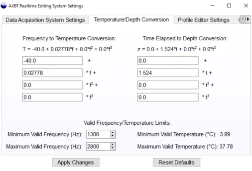
Temperature/Depth Conversion Equation Settings

ARES includes the ability to use customized linear, quadratic, or cubic conversion equations for AXBTs (Fig. 3-3). Two columns are provided: one for frequency-to-temperature and the other for time-to-depth conversions. To adjust the conversion equations being used, enter the coefficient for each term in its respective box. The equation at the top of the respective column should update to reflect the coefficients in the boxes. If non-numeric characters are entered, the equation will not update. The equations used by ARES will not be updated until “Apply Changes" is selected. Additionally, if the contents of the input boxes do not match their respective equations (e.g. due to a non-numeric character as described above), the coefficients used by ARES are based on the equations at the top of each column, not the contents of the input boxes.

Finally, at the bottom of the tab there are two additional inputs to select the valid frequency range. The default range of frequencies ARES accepts as valid AXBT signal is 1300 Hz to 2800 Hz, corresponding to approximately -3.9𝑜_{C to 37}𝑜_{C. However,} because ARES may be used in locations where only a subset of these temperatures are expected (e.g. an AXBT launched in the Southern Ocean during austral winter would most likely not observe 20𝑜C ocean temperatures), this input can be used to apply more precise constraints on the peak frequencies (and therefore temperatures) that ARES accepts as valid observations.

(39)

Figure 3-3: The ARES temperature/depth conversion equation settings window.

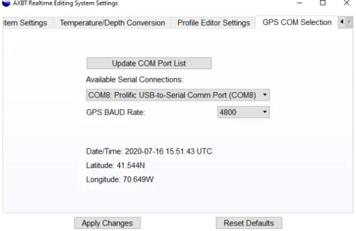
GPS Configuration Settings

The GPS settings tab allows the user to select a serial port for ARES to open and collect GPS data in order to autopopulate drop latitude and longitude when process-ing is started (more information on the GPS NMEA stream and serial configuration is provided in Section 3.2.3). The dropdown menu lists all available serial interfaces (it is worth reiterating that all available interfaces are listed, not just those that are transmitting valid GPS NMEA data streams). If multiple ports are available and the correct port is unknown, the user can try connecting to each port one at a time. If an active GPS receiver is connected to the selected port, this will populate the most recent GPS fix from that receiver. Otherwise, a warning message will appear stating that a GPS data stream could not be identified.

3.2 Procedural Overview

In order to be processed by ARES, VHF data received by an appropriate antenna are demodulated by a WiNRADIO receiver into pulse code modulated (PCM) data (collected at 64 kHz) before being transferred to the computer and appended to a

(40)

Figure 3-4: The ARES GPS configuration settings window.

length-conserving buffer containing one second of data (as new data are appended to the tail of the buffer, an equal number of points are removed from the head). All signal processing and subsequent operations are carried out on PCM data that has been appended to this signal processing thread. All operations prior to PCM data being appended to the Data Acquisition System thread are described in detail in Section 3.2.1, and all following computations are discussed in Section 3.2.2.

3.2.1 Radio Receiver Integration

External Hardware Configuration

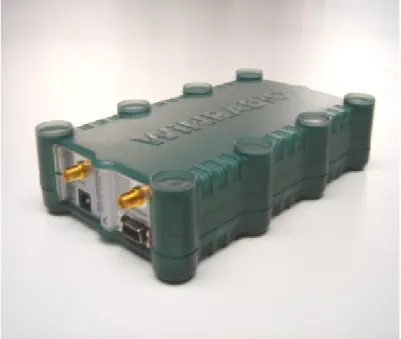
The software-defined radio receiver currently integrated with ARES is a WiNRA-DIO WR-G39WSBe Sonobuoy Receiver (Fig. 3-5; www.winradio.com/home/g39wsbe. htm). It demodulates transmitted signals from standard sonobuoy VHF carrier fre-quencies between 136 and 173.5 MHz, and outputs analog (SMA) and digital (serial) demodulated data. A single receiver weighs 0.43 kg, measures 16.6 cm x 9.7 cm x 4.1 cm, and requires 12V direct current at 0.5A. The receiver has four connections: power (standard 2.5 mm jack), VHF in (SMA male), analog out (SMA male; unused in this application), and digital out (serial). A serial-to-USB converter for the digital

(41)

Figure 3-5: A WiNRADIO G39WSBE software-defined receiver (image from www. winradio.com/home/g39wsbe.htm). Ports on the front-left face of the receiver are: (top left) analog audio out (SMA), (top right) VHF in (SMA), (bottom left) power (2.5 mm), and (bottom right) digital audio out (serial).

output enables easy integration with most modern computers.

A single receiver can only demodulate one VHF frequency at a time, and thus only process good data from one AXBT at a time (although there is potential for an advanced system to track multiple peaks in spectral density simultaneously, this is extremely prone to errors and thus limiting operations to one AXBT per channel at a time is optimal). The time from launch it takes a single AXBT to fully transmit (approximately 11.5 minutes from 10,000 feet, including 120 seconds fall time and an approximately 1.5 𝑚𝑠−1 descent rate to 850 m), constrains the spatial resolution at which AXBTs can be launched as a function of aircraft ground speed. Thus, ARES was configured for the operation of up to six receivers in parallel (though this may be further limited by computer clock rate and random access memory).

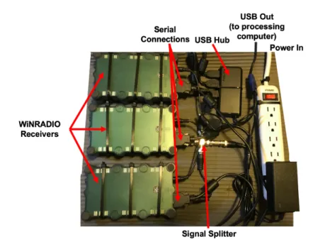
An example of an array of WiNRADIO receivers is shown in Fig. 3-6. This array included three radio receivers that connect to a processing computer via a single USB connection with an unpowered USB hub (with a fourth port available for a GPS receiver). The included power adapter converts standard AC current to 2A 12V DC,

(42)

Figure 3-6: The WiNRADIO receiver array used in this study.

and thus a single adapter was used with a three-way splitter to provide power to all three WiNRADIOs. Additionally, a BNC splitter was used to connect a single VHF antenna output to all three receivers. SMA-to-BNC converters were used for the VHF input to connect the WiNRADIO’s SMA input to this splitter and thus the aircraft’s VHF antenna. In testing, no significant drop in signal level or corresponding processor performance was observed when using the BNC splitter. This configuration of three receivers enabled deployment of deep-water AXBTs (rated to 850m) every 3-4 minutes, or shallow-water AXBTs (rated to 400m) every 2 minutes.

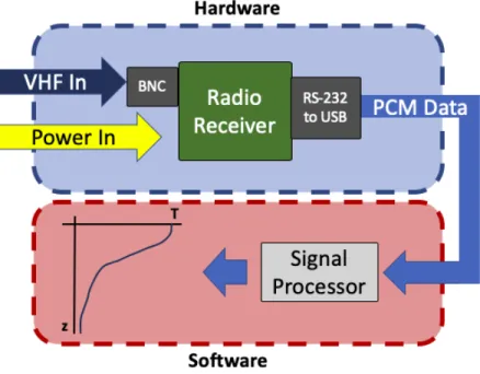
Hardware systems accompanying ARES (following the design of the example ar-ray) require three connections: a standard 60Hz/110V input alternating current wall power supply, a BNC coaxial connection to a VHF antenna for RF signal input, and USB output connected to the processing computer running an instance of ARES. VHF signal received by the connected antenna are demodulated by the WiNRA-DIO receiver, which outputs stream of PCM data collected at 64 kHz from a serial port. This data is transferred to the processing computer using a serial to USB converter and appended to a buffer on the computer using the receiver’s application-programming interface. This buffer is periodically accessed by the ARES Data

(43)

Ac-Figure 3-7: Process to demodulate a received AXBT VHF signal and generate the encoded temperature-depth profile.

quisition System interface to generate a temperature-depth profile from the received data stream (Fig. 3-7).

WiNRADIO API Interaction

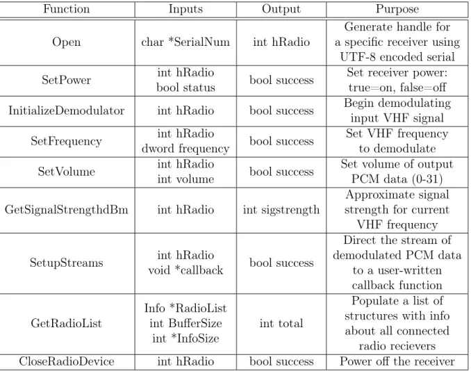
In addition to the required proprietary system drivers (which currently exist for Windows only), a dynamic-link library (DLL) provides the application-programming interface (API) necessary for the processing computer to communicate with and con-trol the WiNRADIO receivers. This was used in conjunction with the Python ctypes module [16] to handle all receiver communication and control exclusively in Python. This API includes a large range of functions for receiver communication and con-trol (an exhaustive list is available at www.winradio.com/home/g39wsb_sdk.htm). While the exact API functions used by the data acquisition system would vary when integrated with a different brand of software-defined receiver, the format would be similar and all operations after demodulated PCM data is accessed by the processing computer would be identical.

The WiNRADIO API is accessed by Python using the ctypes module following the syntax in the example below:

(44)

1 w r d l l = c t y p e s . w i n d l l . L o a d L i b r a r y (’ path - to - DLL - file ’)

Here, wrdll is a class with a library of nested API functions imported from the DLL file. This library includes a large range of functions for receiver communication and control (an exhaustive list is available at http://winradio.com/home/g39wsb_ sdk.htm), but the primary functions used in ARES are listed in Table 3.1.

Table 3.1: WiNRADIO application-programming interface functions integrated in the ARES Data Acquisition System.

Function Inputs Output Purpose

Open char *SerialNum int hRadio

Generate handle for a specific receiver using

UTF-8 encoded serial

SetPower int hRadio

bool status bool success

Set receiver power: true=on, false=off

InitializeDemodulator int hRadio bool success Begin demodulating

input VHF signal

SetFrequency int hRadio

dword frequency bool success

Set VHF frequency to demodulate

SetVolume int hRadio

int volume bool success

Set volume of output PCM data (0-31)

GetSignalStrengthdBm int hRadio int sigstrength

Approximate signal strength for current

VHF frequency

SetupStreams int hRadio

void *callback bool success

Direct the stream of demodulated PCM data to a user-written callback function GetRadioList Info *RadioList int BufferSize int *InfoSize int total Populate a list of structures with info about all connected

radio recievers

CloseRadioDevice int hRadio bool success Power off the receiver

Before passing input arguments to functions nested in the library, Python vari-ables must be converted to C-type varivari-ables (e.g. 16-bit signed integer, unsigned long integer, character array pointer) using the ctypes module. After these conversions, executing commands from the DLL file is straightforward. An example is provided in Appendix C.3.1 demonstrating use of the API-defined function "Open" to access a connected receiver. This requires a pointer to a null-terminated, utf-8 encoded

(45)

char-acter array containing the serial number for the receiver to be activated, and returns an integer handle used as an input argument for all subsequent commands interacting with that receiver.

In order to control multiple receivers, ARES uses the API-defined function "Ge-tRadioList", which provides information about all connected receivers. This function requires a preallocated array of c-type structures (described ind detail on the WiN-RADIO website), with empty fields to be populated by the API. Implementation of this function in a Python environment is demonstrated in Appendix C.3.1.

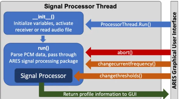
To enable simultaneous processing of multiple AXBTs from multiple receivers in parallel, the ARES Data Acquisition System handles the data stream from each radio (and all associated computations) as individual threads, and uses PyQt’s multithread-ing support to handle processmultithread-ing. Integration of multithreadmultithread-ing is discussed further in Section 3.2.3, but it is worth noting here that each thread is a class with nested functions, as shown in Fig. 3-8. The __init__() function saves all input variables (e.g. Data Acquisition System settings) to the class, and either opens and initial-izes the selected radio receiver if processing data live, or opens and reads in PCM data from a selected WAV file if reprocessing from raw audio. The run() function starts selecting segments of PCM data either using the most recent data received from the WiNRADIO or sequential segments from a source audio file, and process-ing them as described in Section 3.2.2. The changecurrentfrequency() function (only applicable when processing in realtime from a receiver) changes the VHF chan-nel that the receiver is demodulating while it is actively demodulating data. Finally, changethresholds() adjusts the Data Acquisition System settings if the user changes them while the current thread is active and abort() allows the user to terminate the current thread and finish processing.

A WiNRADIO API function, ’SetupStreams’, is used to control PCM data transfer from the receiver to the processing computer. This assigns a callback function that is executed every time a buffer is filled (16-bit PCM data is collected at 64 kHz in a 2 KB buffer, so this occurs at approximately 30 Hz). In ARES, this callback function appends the data to both a WAV file and a buffer on the computer from which PCM

(46)

Figure 3-8: Diagram of nested functions in the ARES Data Acquisition System thread class, with functions listed on arrows using PyQt signals (arrows out of the Data Acquisition System thread block) and slots (arrows into the thread block) to pass information to and from the ARES user interface.

segments are pulled by the data acquisition system and analyzed, following Fig. 3-9. An example of the callback function declaration with SetupStreams is also provided in Appendix C.3.1.

3.2.2 Data Flow

Whether PCM data are read from a WAV file or accessed realtime from a con-nected VHF receiver, the subsequent signal processing sequence is identical. First peak frequency, signal level, and signal-to-noise ratio are determined using a discrete Fourier transform of each segment of tapered PCM data, and then these values are used to infer the temperature-depth profile observed by the AXBT (Fig. 3-9).

Signal Processing

Peak frequency, which is empirically related to the AXBT-observed ocean tem-perature, is determined by applying fast Fourier transforms to small subsets of data. Unless otherwise specified, a window length of 0.3 seconds is used (the effects of

(47)

Figure 3-9: Sequence to pull and process segments of PCM data to identify valid temperature-depth measurements transmitted from an AXBT.

this window length are considered in the ARES Data Acquisition System evaluation section). Before a data subset is transformed into the frequency domain, a cosine (Tukey) taper is applied to the time series in order to minimize spectral leakage (Eq. 3.1). The taper window (𝑇 ) is determined by the length of the PCM data subset (𝐿) and a single parameter (𝛼). The alpha parameter is the ratio of the tapered component of the time series to the total length of the time series, and is constrained by 0 ≤ 𝛼 ≤ 1. 𝑇 [𝑖] = ⎧ ⎪ ⎪ ⎪ ⎪ ⎪ ⎨ ⎪ ⎪ ⎪ ⎪ ⎪ ⎩ 1 2 [︁ 1 + 𝑐𝑜𝑠(︁2𝜋_𝛼 _𝐿−1𝑖−1 − 𝜋)︁]︁, 𝑖 < 𝛼₂(𝐿 − 1) + 1 1 2 [︁ 1 + 𝑐𝑜𝑠(︁2𝜋_𝛼 − 2𝜋 𝛼 𝑖−1 𝐿−1 − 𝜋 )︁]︁ , 𝑖 > 𝐿 − 𝛼₂(𝐿 − 1) 1, otherwise (3.1)

The frequency spectra for a given segment of PCM data are calculated using a fast Fourier transform (requiring only the PCM data subset and corresponding sampling frequency), using the numpy.fft.fft() function included in Python’s Numpy module [17]. The transform of a discrete time series (𝑠, of length 𝐿 and sampling frequency 𝑓𝑠) into the frequency domain (𝑆) is described in Eq. (3.2), where 𝑚 and 𝑛 are discrete indices corresponding to elements in the time and frequency domains, respectively.

(48)

𝑆[𝑛] = 𝐿−1 ∑︁ 𝑚=0 𝑠𝑚𝑒−𝑖2𝜋𝑚𝑛/𝐿, 𝑛 = 0, 1, 2, ...,𝐿 2, ∆𝑓 = 𝑓𝑠 𝐿, 𝑓 = 𝑛∆𝑓 (3.2)

Resulting frequency spectra (𝑆) are collapsed into three characteristic parameters: the peak frequency (𝑓𝑃) and the corresponding signal level (𝑆𝑃) and signal-to-noise ratio (𝑅𝑃; defined mathematically in Eq. 3.3). Only signals from 1300-2800 Hz, corresponding to a realistic temperature range of -3.88𝑜_{C to 37.7}𝑜_{C, are considered.} The signal level depends on the maximum spectral value in the 1300-2800 Hz band (corresponding to the peak frequency that the AXBT is presumed to be transmitting), and the signal-to-noise ratio (SNR) is the ratio of that maximum spectral value in the 1300-2800 Hz band to the maximum value in the entire band. Thus, the SNR ranges between 0 and 1, where it is 0 if no nonzero values are measured in the 1300-2800 Hz band and 1 if the most powerful received signal is in the 1300-1300-2800 Hz band. These parameters are used to distinguish AXBT signal from noise and to calculate the corresponding temperature if necessary. To be considered a valid AXBT signal, the signal level and SNR must both satisfy pre-set thresholds (appropriate thresholds are considered in the Data Acquisition System evaluation). Because possible maximum values of the signal spectra span several orders of magnitude, the peak signal level is expressed in decibels (dB re 1 bit, referenced in this study hereafter as dB).

𝐾 = arg max 𝑆𝑘, 𝑓 [𝑘] ∈ [1300, 2800] (3.3a)

𝑓𝑃 = 𝑓 [𝐾] (3.3b) 𝑆𝑃 = 10log10 (︃ 𝑆[𝐾] 1 bit )︃ (3.3c) 𝑅𝑃 = 𝑆[𝐾] max 𝑆 (3.3d)

(49)

Temperature-Depth Conversion

For signals that satisfy the minimum signal level, frequency range, and SNR re-quirements, temperature and depth are determined from the peak frequency and elapsed time between the current observation and first observation. ARES uses the general empirical relationship between measured temperature (𝑜_{C) and transmitted} frequency (Hz) (Eq. 3.4; noting that the coefficients 1440 and 36 have units of Hz and Hz 𝑜_𝐶−1_{, respectively) and standard fall rate, 1.52 𝑚𝑠}−1 _[6].

𝑓𝑃 = 1440 + 36𝑇 (3.4)

Thus, given the peak frequency (𝑓𝑃) and elapsed time (∆𝑡) since the first observa-tion (when it is presumed the probe is at the surface), the corresponding temperature (𝑇 ) and depth (𝑧, positive down) are calculated as:

𝑇 = −40 + (2.778𝑥10−2)𝑓 (3.5a)

𝑧 = 1.52∆𝑡 (3.5b)

Determining time elapsed requires tracking when the first valid signal was recorded. Because AXBT signals are typically stronger when transmission begins and decay over time as distance between the float and the aircraft increases, in order to prevent VHF interference from prematurely triggering the profile, higher minimum signal level and signal-to-noise ratio thresholds are required for a signal to be accepted as the surface value. Thus, AXBT profiles are processed by repeating the six steps below at the data acquisition system’s sampling frequency of approximately 10 Hz (this process is represented visually in Fig. 3-9):

1. A subset of PCM data is pulled from the input data stream and tapered.

2. The tapered PCM subset is transformed into the frequency domain.

(50)

4. If the signal level and SNR are above the minimum thresholds and profile collec-tion has already been triggered, time elapsed is calculated and the corresponding temperature and depth values are determined and recorded.

5. If profile collection has not been triggered but the signal level and SNR satisfy the trigger thresholds, the observation time is recorded to determine future elapsed times, profile collection is triggered, and the surface temperature is calculated and recorded.

3.2.3 Additional Features

GPS Integration

In order to reduce potential for error by manual entry, ARES was designed to accept input from any GPS receiver that transfers information with a NMEA stream to automatically record position. This is accomplished using Python’s pyserial and pynmea2 modules, which were developed to manage serial data connections and parse GPS NMEA-formatted data, respectively. Using pyserial, ARES scans for and pro-vides a list of all available serial ports. Given a user-specified port, ARES can open the port, parse incoming NMEA data and record latitude and longitude (as long as the selected port is connected to a GPS with a valid NMEA stream), either when data recording is started or to test the connection to a GPS receiver. Examples of using pyserial to retrieve a list of available serial ports (potential GPS receiver connections) and parsing NMEA feed information including time and position from a connected serial port are provided in Appendix C.3.1.

File Types

Raw data from a processed profile can be saved in one of five formats: raw audio (WAV), ASCII signal data, LOG, EDF, and NVO files. WAV files are the most raw form of data available, and recording WAV files is advantageous as it enables reprocessing the profile using different signal processing schemes. However, while some filesystems record creation and “last modified" datetimes, WAV files cannot

(51)

store drop metadata such as time and position. In ARES, temporary WAV files are generated when a receiver is activated, and PCM data is constantly appended to the file as the WiNRADIO continues passing data to the processing computer.

The ASCII signal data file records time elapsed, peak frequency, signal level, and signal-to-noise ratios in a comma-delimited format (in that order). This enables pro-file testing and adjustments (e.g. changes to conversion equations or minimum signal thresholds) without repeating the computationally-expensive signal processing neces-sary to generate a time series of peak frequencies and accompanying signal levels from a source audio file. Like the WAV file, temporary signal data files are created when a receiver is activated and continuously updated as more data is streamed from the receiver. For both the raw audio and signal data files, when the user "saves" the file, they are simply renaming and moving those files from a temporary directory managed by the processing computer’s operating system (e.g. Wondershare for Windows 10).

Finally, the LOG, EDF, and NVO files are all various ASCII file formats for storing the raw data. LOG files are columnar ASCII files including time elapsed, depth, peak frequency, and temperature, but do not include position information. EDF and NVO files include the observed temperature-depth profile as well as time and position information, and the option for additional metadata (e.g. drop number, AXBT type, and additional information). An NVO file format example is provided in Section 4.1.5. When these files are saved by the users, text files are actually generated from the raw profile information stored within the program’s primary class.

Multithreading

The AXBT Realtime Editing System uses multithreading to facilitate processing data from multiple AXBTs simultaneously (either in realtime or from raw audio files). Multithreading and multiprocessing are two methods for handling parallel computa-tions. Multiprocessing requires a central processing unit (CPU) that has multiple cores, each of which are able to run computations simultaneously and separately from one another. Multithreading only requires one core, but instead manages multi-ple threads (individual tasks) that operate simultaneously from the user’s perspective

Development and testing of the AXBT Realtime Editing System (ARES)

Development and Testing of the AXBT Realtime

Editing System (ARES)

by

Lieutenant Junior Grade Casey R. Densmore,

United States Navy

B.S., United States Naval Academy (2018)

Submitted to the Department of Earth, Atmospheric

and Planetary Sciences

in partial fulfillment of the requirements for the degree of

Master of Science in Physical Oceanography

at the

MASSACHUSETTS INSTITUTE OF TECHNOLOGY

and the

WOODS HOLE OCEANOGRAPHIC INSTITUTION

September 2020

c

○2020 Casey R. Densmore.

All rights reserved.

The author hereby grants to MIT and WHOI permission to reproduce

and to distribute publicly paper and electronic copies of this thesis

document in whole or in part in any medium now known or hereafter

created.

Author . . . .

Department of Earth, Atmospheric and Planetary Sciences

August 13, 2020

Certified by . . . .

Steven R. Jayne

Senior Scientist

Woods Hole Oceanographic Institution

Thesis Supervisor

Accepted by . . . .

Glenn R. Flierl

Chairman, Joint Committee for Physical Oceanography

Massachusetts Institute of Technology

Development and Testing of the AXBT Realtime Editing

System (ARES)

by

Lieutenant Junior Grade Casey R. Densmore,

United States Navy

Abstract

Acknowledgments

Contents

List of Figures

List of Tables

Chapter 1

Introduction

1.1

Motivation

1.2

TROPIC Program Background

1.3

Contribution and Organization

Chapter 2

Background

2.1

AXBT System Overview

2.2

AXBT Processing

2.2.1

Data Acquisition

2.2.2

Empirical Conversion Equations

2.2.3

AXBT Profile Quality Control

Chapter 3

ARES Data Acquisition System

3.1

Data Acquisition System Interface Description

3.1.1

Layout

3.1.2

Settings

3.2

Procedural Overview

3.2.1

Radio Receiver Integration

3.2.2

Data Flow

3.2.3