the N
H i
− Z Distribution
Jens-Kristian Krogager
1
, Palle Møller
2
, Lise B. Christensen
3
, Pasquier Noterdaeme
1
,
Johan P. U. Fynbo
3
, Wolfram Freudling
2
1Institut d’Astrophysique de Paris, CNRS-SU, UMR7095, 98bis bd Arago, FR-75014 Paris, France; E-mail: [email protected] 2European Southern Observatory, Karl-Schwarzschildstrasse 2, D-85748 Garching bei München, Germany
3DARK, Niels Bohr Institute, University of Copenhagen, Lyngbyvej 2, DK-2100 Copenhagen Ø, Denmark
19 May 2020
ABSTRACT
We investigate how damped Lyman-α absorbers (DLAs) at z ∼ 2 − 3, detected in large optical spectroscopic surveys of quasars, trace the population of star-forming galaxies. Building on previous results, we construct a model based on observed and physically motivated scaling relations in order to reproduce the bivariate distributions of metallicity, Z, and H i column den-sity, NH i. Furthermore, the observed impact parameters for galaxies associated to DLAs are in agreement with the model predictions. The model strongly favours a metallicity gradient, which scales with the luminosity of the host galaxy, with a value of γ∗= −0.019 ± 0.008 dex kpc−1 for L∗ galaxies that gets steeper for fainter galaxies. We find that DLAs trace galaxies over a wide range of galaxy luminosities, however, the bulk of the DLA cross-section arises in galaxies with L ∼ 0.1 L∗at z ∼ 2.5 consistent with numerical simulations.
Key words: galaxies: high-redshift — galaxies: statistics — quasars: absorption lines
(e.g.Pontzen et al. 2008;Altay et al. 2013;Bird et al. 2013,2014, 2015;Rahmati & Schaye 2014). However, the redshift evolution and the details of the bivariate distribution of NH iand Z are still not
well-understood (Hassan et al. 2020) and the properties of DLAs in simulations depend strongly on the rather ad-hoc feedback mecha-nisms from supernovae and quasars assumed in the simulations.
Another way to study DLA galaxy properties is by cross-correlation analyses with Lyα forest absorbers in order to measure the DLA bias, bdla (Font-Ribera et al. 2012;Pérez-Ràfols et al.
2018a). Based on a large statistical analysis,Pérez-Ràfols et al. (2018a) find an average bias of bdla= 2.0 ± 0.1, which translates
to a rather large halo mass (∼ 1011M ) if all DLAs reside in halos
of the same mass; However, the inferred DLA halo mass depends on the distribution function for DLA cross-section as a function of halo mass. A power-law scaling between DLA cross-section and halo mass with index larger than unity implies that DLAs instead reside in a large range of halo masses, where the minimum mass depends critically on the assumed power-law index (Pérez-Ràfols et al. 2018a). Moreover, the inferred bdla depends on metal line
strength (Pérez-Ràfols et al. 2018b) indicating that more metal-enriched DLAs reside in more massive halos, consistent with the mass–metallicity relation inferred for DLAs (Møller et al. 2013; Christensen et al. 2014).
The most direct method to examine the galaxies associated to DLAs is through direct detections (see compilation byMøller & Christensen 2020). Yet, detections of high-z DLA-galaxies have been scarce due to their intrinsically faint nature (Fynbo et al. 1999; Haehnelt et al. 2000;Schaye 2001;Krogager et al. 2017). Recently,
1 INTRODUCTION
The properties of neutral gas are crucial for a complete understand-ing of galaxy evolution. Locally, the neutral gas can be studied directly through the H i 21-cm transition (e.g., Zwaan et al. 2005; Walter et al. 2008). At high redshift the neutral gas phase is best studied through Lyα absorption towards background quasars. The so-called damped Lyα absorbers (DLAs) with NH i > 2×1020 cm−2
are of particular interest for studies of galactic environments (Wolfe et al. 2005). Due to their high column density of neutral hydrogen, DLAs arise in predominantly neutral gas (Viegas 1995). As a result, ionization corrections for metallicity measurements are negligible.
The distribution function of NH i for DLAs, f (NH i), has been studied in detail (Prochaska & Wolfe 2009; Noterdaeme et al. 2012; Bird et al. 2017) and provides a measurement of the cosmic mass density of neutral hydrogen in DLAs, Ωdla. It is found that Ωdla
makes up ∼80 % of the total mass density of H i at z > 2.2 ( Noter-daeme et al. 2009).
The plethora of low-ionization metal absorption lines make it possible to obtain accurate measurements of the metallicity, Z, in the neutral gas (Rafelski et al. 2012; Jorgenson et al. 2013; De Cia et al. 2018). It is found that the average Z increases towards lower redshifts in agreement with expectations from the build up of metals via star formation (Dvorkin et al. 2015).
In order to properly interpret the properties of DLAs it is im-portant to know which galaxies give rise to DLAs over cosmic time. One way to understand the galaxy population associated to DLAs is through numerical simulations. Large cosmological simulations are able to match the observables from DLAs at z ≈ 3 fairly well
however, powerful integral field spectrographs enable more effec-tive follow-up of DLA-galaxies by probing large areas around the background quasar (Fumagalli et al. 2017).
Since we only observe the brightest DLA-galaxies, it is nec-essary to extrapolate from the individual associations to obtain the global properties of DLAs.Fynbo et al.(2008) have carried out a successful modelling approach to reproduce the Z and impact pa-rameter distribution of DLAs at z ≈ 3.Padmanabhan & Refregier (2017) have studied the H i distribution of DLAs using an analyti-cal formalism to link halo properties to H i mass and cross-section. Their model reproduces well the redshift evolution of dndla/dz but
overproduces the number of high NH isystems.
While the models byFynbo et al.(2008) andPadmanabhan & Refregier (2017) are successful at predicting the distributions of Z and NH iindependently, so far there have been no attempts
to model both of these key properties simultaneously. Here we therefore extend the original model byFynbo et al.(2008) to include a statistical prescription for NH iin order to describe the bivariate
NH i-Z distribution. We furthermore include the effects of a dust bias in optical quasar selection affecting the observed DLA properties (Pei et al. 1991;Murphy & Bernet 2016;Krogager et al. 2019). In this paper, we perform a Bayesian analysis to constrain the model parameters including priors on parameters that have already been constrained independently.
The paper is organized as follows: In Sect.2, we describe the compilation of data used to constrain the model; in Sect. 3, we present the details of our model and the parameter estimation; We discuss the results and implications of our work in Sect. 4; and lastly, we summarize our findings in Sect.5.
Throughout this paper, we assume a flat ΛCDM cosmology with H0 = 68 kms−1Mpc−1, ΩΛ = 0.69 and Ωm = 0.31 (Planck
Collaboration et al. 2016).
2 LITERATURE DATA
In order to constrain our model, we use the observed NH i
distri-bution function derived byNoterdaeme et al.(2012) based on a statistical sample of ∼3500 DLAs at redshifts 2 < z < 3 detected in ∼40000 quasar spectra. However, only a small subset of these have robust measurements of metallicity, Z. We compile a sample of Z measurements from the literature combining the three largest samples available byQuiret et al.(2016),Jorgenson et al.(2013) andRafelski et al.(2012). We remove measurements based on limits and those based only on iron as this element tends to deplete heav-ily onto dust grains. We furthermore only consider DLAs in the redshift range 2 < z < 3. This sample of 178 DLAs will hereafter be referred to as the ‘full DLA sample’. The selection effects are discussed in more detail in Sect.4. All values of metallicities are in units of Solar metallicity, Z , unless stated otherwise. We have
corrected all the measurements described above to the same So-lar reference values using measurements byAsplund et al.(2009) and the recommendations byDe Cia et al. (2016) as to whether photospheric or meteoritic values are used.
In order to compare impact parameter predictions from our model, we use the sample of high-redshift (zabs & 2) DLAs with confirmed emission counterparts compiled byMøller & Christensen (2020) andKrogager et al.(2017). We restrict the sample to the subset with log(NH i/ cm−2) >20.3. To this sample, we add three counterparts reported byRanjan et al.(2020) at z ∼ 2.3 together with one DLA counterpart bySrianand et al.(2016) at z = 3.247 and one byFumagalli et al.(2017) at z = 3.25. This sample will hereafter be referred to as the ‘DLA galaxy sample’.
3 MODELLING HIGH-REDSHIFT DLAS
The model described here is based on the work byFynbo et al. (2008). We here offer a short summary of the model framework and refer the reader to the original work for further details. In this work, we only consider redshifts between 2 < z < 3. The model uses a selection probability of DLAs given by Pdla ∝σdlaφ(L), where σdla is the effective cross-section of DLAs and φ is the
UV luminosity function. For the luminosity function, a Schechter function of the form φ(L) = φ0(L/L∗)α exp(−L/L∗)is used.
We assume σdla, given by πR2dla, to scale with luminosity,
through a Holmberg relation Rdla = R∗dla(L/L∗)t, and vanish below a limiting luminosity Lmin. In what follows, all quantities
marked by∗are referring to the given quantity of an L∗galaxy, e.g.,
the radial extent of DLA cross-section for an L∗galaxy is denoted
Rdla∗ . The absolute value of Rdla∗ is obtained by requiring that the incidence rate, dndla/dz, matches the observed value at z ≈ 2.5.
We calculate dn/dz as: dn dz = πR∗dla2φ0c(1 + z)2H−1(z) Z ∞ Lmin Lα+2te−LdL , (1) where L is in units of L∗and the Hubble parameter is given as:
H(z)= H0 q
Ωm(1 + z)3+ ΩΛ. (2)
We here use the observed value of dndla/dz = 0.21±0.04 at z = 2.5
(Zafar et al. 2013).
Galaxies are then sampled from the luminosity function weighted by σdla, and an impact parameter, b, is drawn randomly
with a probability P(b) ∝ b for b ≤ Rdla(L), that is, the probability
is weighted by area.
A central metallicity, Z0is assigned to each galaxy assuming a
metallicity–luminosity (Z−L) relation: log(Z0)= log Z0∗+ β×Muv. A radial metallicity gradient is then assumed in order to obtain a value of the metallicity, Zabs, at the impact parameter where the
absorption system would be observed. This gradient is taken to be luminosity dependent with a variable power-law index: γ = γ∗
Lqz. While the original work byFynbo et al.(2008) assumed a fixed value of qz= −t followingBoissier & Prantzos(2001), we keep this index
as a free parameter in order to quantify whether a universal gradient (i.e., qz= 0) is preferred over a luminosity dependent gradient. 3.1 Including H i and dust
The neutral gas in galaxies is roughly expected to follow an exponen-tial distribution with radius: NH i(r )= NH i, 0exp(−r/rhi)(Walter et al. 2008). The scale length, rhi, is calculated by demanding that
NH i(r= Rdla)= 2 × 1020cm−2. For this reason, rhiis not a free
parameter in this model. The central NH ivalue is however kept as a
free variable with an adopted fiducial value of NH i, 0= 1022cm−2.
Motivated by observations of local H i discs by the THINGS survey (Walter et al. 2008), we include a stochastic term in the radial NH idistribution to account for local fluctuations in column density as well as inclination effects which are not explicitly modelled. The fluctuations are implemented as a log-normal scatter around the smooth average radial profile:
log NH i(r )= log NH i, 0−log(e)
rhi r+ N (0, σhi) , where the log-normal scatter σhi is a free variable in our model
with a fiducial value of 0.3 dex.
Since we now have a prescription for both NH i and Z, we
the absorption sightline, A(V ). This value is obtained following Zafar & Møller(2019) assuming a constant dust-to-metals ratio, log κz= −21.4.
Lastly, we include a dust bias to account for the fact that quasars behind dusty DLAs are systematically under-represented due to the complex colour and magnitude selection criteria. We calculate the selection probability as Pqso = sech(x2), where x = A(V )/A(V )crit. This functional form fits very well the cal-culated selection probability byKrogager et al.(2019) for a value of A(V )crit= 0.25 mag. The model distributions are filtered according
to Pqsoto produce a mock observable model distribution.
In total, the original model contains 9 free parameters: {φ0, M∗
uv, α, Lmin, t, β, γ∗, Z∗, qz}, and with the above mod-ifications, we have effectively added the following 3 parameters: {NH i, 0, σhi, A(V )crit}.
3.2 Constraining model parameters
Due to the significant degeneracies in the parameters we constrain the model parameters using a Bayesian approach. This also allows us to include priors since we have independent constraints on many parameters. For this purpose, we use the Python package Emcee (Foreman-Mackey et al. 2013).
We use the observed distributions of NH iand Z (see Sect.2)
to statistically constrain the model parameters. For a given set of parameters, we draw a large sample of 50,000 DLAs and then calcu-late the model f (NH i)in the same bins as the data, using only DLAs that pass the mock quasar selection as implemented here using Pqso
(see Sect.3.1). The distribution function is normalized by requiring that the integral R∞
Ndla f(NH i)dN matches the observed value of
R∞
Ndla f(NH i)dN, where Ndla = 2 × 10
20cm−2. This
normaliza-over a reasonable range of parameter space. We have verified that the choice of prior ranges do not affect the results and all values are constrained well within the chosen ranges. For the parameters with more restrictive priors, the details of the priors are given below.
We constrain the shape of the luminosity function following observations fromMalkan et al. (2017). The parameters M∗
uv =
−20.9 and φ0= 1.7 × 10⁻³Mpc−3are kept fixed as they agree very well from one survey to another (Malkan et al. 2017, table 3). On the other hand, we choose to keep α as a free parameter since this value shows large dispersion among various surveys. The average value and the standard deviation are used as a prior on α. In this work, we adopt a fiducial value of Lmin= 10−4L∗. This value is consistent with numerical simulations (Bird et al. 2013) and semi-analytical modelling (Dvorkin et al. 2015).
The slope of the Z − L relation, β, is constrained from obser-vations of galaxies at z ∼ 0.5 − 1 (Kobulnicky & Kewley 2004; Hi-dalgo 2017). We obtain an average value of hβi = 0.211(weighted by individual uncertainties) with a standard deviation of 0.05. This average value is taken as our prior and is in agreement with re-sults from previous modelling (Krogager et al. 2017). Although the redshift range studied by Hidalgo(2017) is lower than what we try to model here, there is evidence that the slope of the related mass–metallicity relation does not evolve significantly with redshift (Maiolino et al. 2008). It is therefore reasonable to assume that the slope of the metallicity–luminosity relation would also remain constant with redshift.
The normalization of the Z−L relation, Z∗, is constrained from
observations of the mass–metallicity relation at z ∼ 2.2 (Maiolino et al. 2008). We find that galaxies around M∗have roughly Solar
metallicity. In order to take into account the observed scatter as well as systematics, we use a weak prior on Z∗: log Z∗= 0.0 ± 0.2.
We use a fiducial value of A(V )crit = 0.25 mag, derived
using the calculation of selection probability as a function of A(V ) fromKrogager et al.(2019). The value of 0.25 mag corresponds to a limiting A(V ) of 0.57 mag for a selection probability of PQSO = 0.01, i.e., DLAs with A(V ) larger than 0.57 mag have a selection probability less than 1% in SDSS-II (up until DR7). Since the ‘full DLA sample’ is observed with larger telescopes than the SDSS this A(V ) limit may differ with respect to the fiducial value. We therefore keep this value as a free parameter and assign a rather arbitrary logarithmic uncertainty for the prior of 0.3 dex. The results do not depend strongly on the chosen width of the prior distribution. Using the priors mentioned above, we obtain an initial estimate of the parameters using Emcee to explore parameter space with 100 walkers for 600 steps. The posterior probability distribution shows a strong one-to-one anti-correlation between the parameters t and qzwith a Spearman correlation coefficient of −0.92. A similar anti-correlation is implemented in the original model byFynbo et al. (2008) followingBoissier & Prantzos(2001), who use qz = −t.
Based on the observed anti-correlation we adopt the constraint: qz= −t. Hence, qzis no longer considered a free parameter.
Although the average metallicity gradient of DLA hosts has been inferred byChristensen et al.(2014), we do not include this constraint as a prior on γ∗. Since these authors have assumed a
constant gradient with no luminosity dependence and no separation between low- and high redshift DLA galaxies, including their ob-tained metallicity gradient as a prior in this work could possibly bias our results.
1 Note the change of sign in our definition with respect toHidalgo(2017).
tion ensures a correct absolute scaling of f (NH i) in order to match the observed dndla/dz. We then calculate the likelihood assuming
Gaussian statistics given the uncertainties quoted by Noterdaeme et al. (2012).
Similarly, we obtain a model distribution for Z which we com-pare to the observed distribution using a Kolmogorov–Smirnov (KS) test. Although the p-value from a KS test is not an exact estimator of the formal likelihood, the two are suciently correlated (Krueger & Heck 2017) allowing us to use Pks as an estimate of the likelihood.
In our case we find that the p-value provides tighter constraints than other likelihood estimators (such as kernel density estimators).
Along with the constraints from the NH i and Z distributions,
we have the following independent constraints:
(i) The average reddening for DLAs, which pass the optical quasar selection criteria, hE(B − V )iobs, must not exceed 21 mmag
at the 3-σ level (Murphy & Liske 2004). We use this conservative upper limit since there is significant disagreement among various measurements (see Murphy & Bernet 2016);
(ii) The average metallicity of extremely strong DLAs (ESDLAs, log(NH i) > 21.7, Noterdaeme et al. 2014) is observed to be hZi = −1.30 ± 0.05 (Ranjan et al. 2020).
The joint likelihood is then taken as the product of the indepen-dent likelihoods taking into account the higher number of degrees of freedom for the NH i data.
3.2.1 Priors
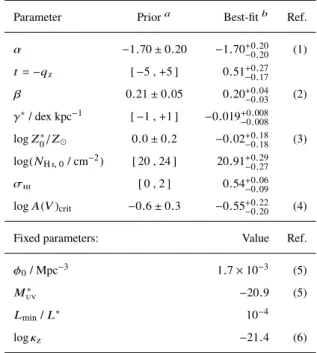
All priors used in our statistical analysis are summarized in Table 1. For parameters where we have no prior knowledge we use flat priors
Table 1. Summary of free model parameters
Parameter Priora Best-fitb Ref.
α −1.70 ± 0.20 −1.70+0.20−0.20 (1) t= −qz [ −5 , +5 ] 0.51+0.27−0.17 β 0.21 ± 0.05 0.20+0.04 −0.03 (2) γ∗/ dex kpc−1 [ −1 , +1 ] −0.019+0.008 −0.008 log Z∗ 0/Z 0.0 ± 0.2 −0.02+0.18−0.18 (3) log(NH i, 0/ cm−2) [ 20 , 24 ] 20.91+0.29 −0.27 σhi [ 0 , 2 ] 0.54+0.06−0.09
log A(V )crit −0.6 ± 0.3 −0.55+0.22−0.20 (4)
Fixed parameters: Value Ref.
φ0/ Mpc−3 1.7 × 10⁻³ (5)
M∗
uv −20.9 (5)
Lmin/ L∗ 10−4
log κz −21.4 (6)
aGaussian priors are given as µ ± σ; Flat priors are given as [min , max]. bBest-fit values are stated as the median value with 16-th and 84-th percentiles as confidence intervals.
References for priors: (1)Malkan et al.(2017); (2)Hidalgo(2017); (3) Maiolino et al.(2008); (4)Krogager et al.(2019); (5)Malkan et al.(2017); (6)Zafar & Møller(2019).
3.3 Results
We obtain the best-fit solution using Emcee with 100 walkers for 800 iterations of which we discard the first 200 iterations for which the ensemble has not converged. The values of the optimized model parameters are given in Table1. These are stated as the median value of the posterior probability distribution together with the 16th and 84th percentiles as 1-σ confidence intervals.
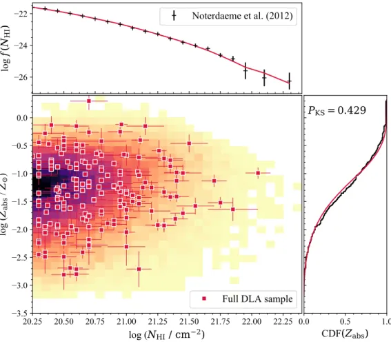
The results of the best-fit model are shown in Fig.1. We find a very good agreement between the model and the data. For compar-ison, we also show the impact parameter distribution as a function of NH iand Z in Fig.2. Since the ‘DLA galaxy’ sample is not
com-plete and suffers from strong and inhomogeneous selection effects (mainly high-metallicity galaxies have been targeted and identified), we do not include the impact parameters in the formal modelling. Nonetheless, it is interesting to compare the model predictions to the observations. We find that the observations indeed overlap with the model predictions which lends qualitative support to the best-fit model, in particular since these observations have not been used to constrain the model parameters.
4 DISCUSSION
4.1 Radial distribution of NH i
The best-fit value of NH i, 0 = 8+8−4×1020cm
−2is consistent with
local H i observations from the THINGS survey who report typical values of ∼ 10 M pc−2 corresponding to ∼ 1021 cm−2 (Walter
et al. 2008). The inferred amount of scatter in log(NH i) is high, σhi = 0.54+0.07
−0.09 dex, compared to the fairly smooth radial
pro-files presented byWalter et al.(2008). This is expected since the
individual radial profiles presented by Walter et al.(2008) have been azimuthally averaged. Moreover, the H i-emission studies pro-vide beam-averaged measurements (typically 100 − 500 pc for the THINGS galaxies) which smoothes out small-scale structure. The very small scales probed by quasar sightlines (.1 pc; e.g, Bala-shev et al. 2011) may therefore show much larger local variations. A large degree of randomness in NH iis also expected since the
neutral medium is highly turbulent (Elmegreen & Scalo 2004) and our model samples the whole galaxy population, not just a single galaxy.
4.2 DLA impact parameters
The distribution of NH iand impact parameter is in qualitative
agree-ment with the simulation byRahmati & Schaye(2014). In order to make a fair comparison, we restrict our model to only consider DLA hosts with similar star formation rates (SFRs) asRahmati & Schaye(SFR > 0.004). For this purpose, we calculate SFR based on the UV luminosity included in our model followingKennicutt (1998), i.e., SFR ∝ Luv. We find that the median impact parameter
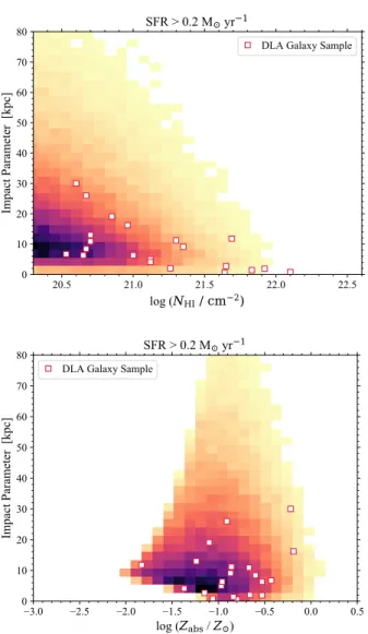
increases when looking at DLA hosts with larger SFRs (see top panel of Fig.3). This is similar to the simulations byRahmati & Schaye(2014), yet the median impact parameters from our best-fit model are ∼2 times larger. The simulations byRahmati & Schaye (2014) do not provide explicit information on the absorption metal-licity and it is therefore not certain whether they match the bivariate NH i-Z distribution.
Our results are in better agreement with the recent simulation byRhodin et al.(2019), who find larger impact parameters for high-redshift absorbers. The observed anti-correlation between log(NH i) and impact parameter is however not recovered at z > 1 in the simulation byRhodin et al.(2019). Their simulation only addresses one Milky Way type progenitor, which is more massive than the average DLA host in our work, and it is therefore difficult to perform a one-to-one comparison between their simulation and our work.
We have also investigated how the metallicity–impact parame-ter distribution varies when considering only DLA hosts with SFR larger than 0.2 M yr−1. This limit corresponds broadly to the SFR
limit obtained in the ‘DLA galaxy sample’. In the lower panel of Fig.3, we show the distribution of impact parameters as a func-tion of absorber metallicity for DLA hosts with SFR larger than 0.2 M yr−1. By restricting the model distribution to this SFR limit
we obtain a good match to the observations. However, it is not possible to quantify the agreement in more detail given the inho-mogeneous sample selection of the DLA galaxy sample, combined with the fact that the detections are based on different emission lines (e.g., Lyα, Hα, [O iii]) yielding inhomogeneous detection limits.
4.3 DLA cross-section and halo properties
In the following, we shall compare the cross-section of DLAs, σdla,
as a function of their host luminosity to results from numerical simulations.Bird et al.(2014) find that σdlaas a function of halo
mass is well-reproduced by a power-law with an index between 0.8 and 1. The upper range of their results is in good agreement with the luminosity scaling we infer for σdlaof 1.02 (σdla ∝ L2t, and t = 0.51) assuming a constant mass-to-light ratio. The normalization of the power-law relation inferred byBird et al.(2014) is ∼ 100 kpc2
at Mh = 1010M . Pontzen et al. (2008) find a steeper relation
for σdlaas function of halo mass for low masses which flattens at
20.25
20.50
20.75
21.00
21.25
21.50
21.75
22.00
22.25
log (
N
HI
/ cm
2
)
3.5
3.0
2.5
2.0
1.5
1.0
0.5
0.0
log (
Z
abs
/
Z
)
Full DLA sample
0.0
0.5
1.0
CDF
(Z
abs
)
P
KS
= 0.429
26
24
22
log
f(N
HI
)
Noterdaeme et al. (2012)
Figure 1. Model prediction for the bivariate NH iand Zabsdistribution. Zabshere refers to the metallicity at the given impact parameter in contrast to the central metallicity, Z0, that would be probed by emission line measures. The colors of the model distribution indicates the number of model points in the given bin normalized to a linear scale from 0 to 1. The marginalized Zabsdistribution is shown in the right panel as the cumulative distribution function (CDF, in black) together with the best-fit model (in red). The top panel shows the NH idistribution function (black points) compared to the best-fit model (red line).
20.5 21.0 21.5 22.0 22.5
log (
N
HI/ cm
2)
0 10 20 30 40 50 60 70 80Impact Parameter [kpc]
DLA Galaxy Sample
3.0 2.5 2.0 1.5 1.0 0.5 0.0 0.5
log (
Z
abs/
Z
)
0 10 20 30 40 50 60 70 80Figure 2. Model prediction for impact parameter as a function of NH i (left) and Zabs (right) for all model galaxies (SFR > 0 M yr−1). The color scale of the model distributions follows that of Fig. 1. The sample of DLA galaxies is shown as open, square points. We note that the ‘DLA galaxy’ sample is neither complete nor representative and hence should only be compared qualitatively to the underlying model distribution.
20.5 21.0 21.5 22.0 22.5 log (
NHI
/ cm
2)
0 10 20 30 40 50 60 70 80 Impact Parameter [kpc]SFR > 0.2 M yr
1DLA Galaxy Sample
3.0 2.5 2.0 1.5 1.0 0.5 0.0 0.5 log (
Zabs
/Z
) 0 10 20 30 40 50 60 70 80 Impact Parameter [kpc]SFR > 0.2 M yr
1 DLA Galaxy SampleFigure 3. Model prediction for impact parameter as a function of NH i(top) and Zabs(bottom) considering only DLA hosts with SFR > 0.2 M yr−1.
their simulation is ∼ 50 kpc2. As our analysis is based on the DLA galaxy luminosity, we need to assume a halo-mass-to-light ratio in order to compare our model to the simulations. The best-fit model yields a characteristic scale of DLA cross-section for a L∗galaxy
of R∗
dla= 31 kpc. In order to reproduce the simulations byPontzen
et al.(2008) andBird et al.(2014), we therefore need to assume Mh/Luv ∼20 − 40 M /L for L∗ galaxies. This Mh/Luv ratio
is consistent with what is found in the literature (Vale & Ostriker 2006;Mason et al. 2015).
We then compare the distribution of DLA galaxy luminosities from our model to the halo mass distribution from the simulations byBird et al.(2014). For our best-fit model, we find that the bulk of the DLA cross-section is contributed by galaxies around 0.1 L∗.
Assuming the average inferred Mh/Luv = 30, we obtain a bulk
halo mass for DLAs of 6 × 10¹⁰ M . This is consistent with the
peak of the halo-mass distribution presented byBird et al.(2014, their fig. 2). The minimum halo mass contributing to the DLA cross-section in the simulations byBird et al.(2014) is Mmin ≈ 109M consistent with modelling studies of the halo properties of
DLAs (e.g.,Pontzen et al. 2008;Barnes & Haehnelt 2009,2014; Padmanabhan & Refregier 2017). Using the Mh–Luv relation by
Mason et al.(2015), we find that a minimum halo mass of 109M
corresponds to Lmin= 4 × 10⁻⁵L∗. This is in good agreement with the fiducial value of Lmin = 10−4 L∗assumed in this work, when taking the significant scatter of the halo mass relations into account. The halo properties of DLA galaxies can furthermore be stud-ied by analysing the cross-correlation of DLAs and Lyα forest ab-sorbers (Font-Ribera et al. 2012;Pérez-Ràfols et al. 2018a). Based on SDSS DR12,Pérez-Ràfols et al.(2018a) find that the observed bias is consistent with a minimum halo mass of Mmin∼109M if
the DLA cross-section scales with halo mass as a power-law with index a ≈ 1.05. This might be slightly at odds with the lower range of the power-law index inferred byBird et al.(2014) although not ruled out. It is on the other hand consistent with the results of our model within the rather large uncertainty on t.
4.4 Metallicity gradients
The best-fit value of the metallicity gradient for L∗ galaxies,
γ∗= −0.019 ± 0.008 dex kpc−1, is in good agreement with the
pre-vious measurements of the average metallicity gradient for DLAs of γ = −0.022 ± 0.004 (Christensen et al. 2014). This agreement is consistent with the fact that most of the high-redshift galaxies analysed byChristensen et al. (2014) are fairly bright and have luminosities around L∗. Similar estimates are reported byPéroux
et al.(2012), although the scatter among individual measurements is significant. When studying emission-selected galaxies at z & 1, a large range in metallicity gradients has been observed in galaxy discs (e.g.,Swinbank et al. 2012;Stott et al. 2014;Curti et al. 2020). Curti et al.(2020) report flat or negative gradients for the major-ity of galaxies, and only in a few cases do they observe inverted metallicity gradients (i.e., more metal-rich at larger radii). The au-thors find a slight trend of steeper, negative metallicity gradients for more massive galaxies, contrary to the relation found in our model, where the metallicity gradient flattens for more luminous (and thus massive) galaxies; γ ∝ L−0.5. This disagreement might however be
a result of sample selection effects together with the very different ways by which metallicity gradients are measured in absorption and emission as well as the physical scales they probe.
The study byCurti et al.(2020) has very few galaxies at z > 2, and all of these are highly star-forming (SFR ∼ 50 M yr−1) and rather
massive (M? ∼1010M ). DLA hosts in our model probe faint
galaxies with low star-formation activity corresponding to stellar masses in the range of . 109 M . It is thus plausible that the
differences derived in the luminosity (or mass) dependence is due to the very different sample characteristics in terms of stellar mass. We furthermore note that while luminosity and mass are correlated, it is not a one-to-one correspondence due to variations in star-formation histories and dust attenuation.
Beyond sample selection effects, the emission samples further present a mix of various emission line diagnostics which have com-plicated systematic effects (e.g.,Kewley & Ellison 2008). In studies combining emission and absorption, similar systematic effects come into play (seePéroux et al. 2012;Rahmani et al. 2016). Lastly, the observations of high-redshift galaxies in emission only probe the in-ner few kpc of the brightest galaxies. In contrast, our analysis takes into account the average metallicity gradient of the whole DLA galaxy population out to large distances. We thus conclude that the metallicity gradient for DLA galaxies included in our model is not directly comparable to the observed emission-line-derived metal-licity gradients, and any differences might therefore be ascribed to differences in sample selection and methodology. Further investiga-tion is needed to analyse these systematics in detail; However, this is beyond the scope of this work.
By converting the UV luminosities in our analysis to halo masses (followingMason et al. 2015), we compare the distribution of DLA galaxy luminosities in our model to the halo mass dis-tribution seen in numerical simulations (Pontzen et al. 2008;Bird et al. 2014). We find that the model distribution is consistent with numerical simulations in terms of cross-section and its scaling with luminosity (halo mass) as well as the lower luminosity (mass) limit for DLA cross-section of ∼ 10−4L∗(∼ 109M
).
Lastly, we find strong evidence for a negative radial metallicity gradient which scales inversely with luminosity, i.e., more luminous galaxies have flatter gradients. While this trend with luminosity is somewhat at odds with the mass dependence seen in observations (e.g.,Curti et al. 2020), the average value of the gradient for L∗
galaxies, γ∗ = −0.019 ± 0.008 dex kpc−1, is in agreement with
other works (Christensen et al. 2014;Stott et al. 2014).
ACKNOWLEDGEMENTS
We thank the anonymous referee for the very constructive report. We would like to thank Matt Lehnert for fruitful discussions. The research leading to these results has received funding from the French Agence Nationale de la Recherche under grant no ANR-17-CE31-0011-01 (project “HIH2” – PI Noterdaeme).
REFERENCES
Altay G., Theuns T., Schaye J., Booth C. M., Dalla Vecchia C., 2013,
MNRAS,436, 2689
Asplund M., Grevesse N., Sauval A. J., Scott P., 2009,ARA&A,47, 481
Balashev S. A., Petitjean P., Ivanchik A. V., Ledoux C., Srianand R., Noter-daeme P., Varshalovich D. A., 2011,MNRAS,418, 357
Barnes L. A., Haehnelt M. G., 2009,MNRAS,397, 511
Barnes L. A., Haehnelt M. G., 2014,MNRAS,440, 2313
Bird S., Vogelsberger M., Sijacki D., Zaldarriaga M., Springel V., Hernquist L., 2013,MNRAS,429, 3341
Bird S., Vogelsberger M., Haehnelt M., Sijacki D., Genel S., Torrey P., Springel V., Hernquist L., 2014,MNRAS,445, 2313
Bird S., Haehnelt M., Neeleman M., Genel S., Vogelsberger M., Hernquist L., 2015,MNRAS,447, 1834
Bird S., Garnett R., Ho S., 2017,MNRAS,466, 2111
Boissier S., Prantzos N., 2001,MNRAS,325, 321
Christensen L., Møller P., Fynbo J. P. U., Zafar T., 2014,MNRAS,445, 225
Curti M., et al., 2020,MNRAS,492, 821
De Cia A., Ledoux C., Mattsson L., Petitjean P., Srianand R., Gavignaud I., Jenkins E. B., 2016,A&A,596, A97
De Cia A., Ledoux C., Petitjean P., Savaglio S., 2018,A&A,611, A76
Dvorkin I., Silk J., Vangioni E., Petitjean P., Olive K. A., 2015,MNRAS,
452, L36
Elmegreen B. G., Scalo J., 2004,ARA&A,42, 211
Font-Ribera A., et al., 2012,J. Cosmology Astropart. Phys.,11, 59
Foreman-Mackey D., Hogg D. W., Lang D., Goodman J., 2013,PASP,125, 306
Fumagalli M., et al., 2017,MNRAS,471, 3686
Fynbo J. U., Møller P., Warren S. J., 1999, MNRAS,305, 849
Fynbo J. P. U., Prochaska J. X., Sommer-Larsen J., Dessauges-Zavadsky M., Møller P., 2008,ApJ,683, 321
Haehnelt M. G., Steinmetz M., Rauch M., 2000,ApJ,534, 594
Hassan S., Finlator K., Davé R., Churchill C. W., Prochaska J. X., 2020,
MNRAS,492, 2835
Hidalgo S. L., 2017,A&A,606, A115
Jorgenson R. A., Murphy M. T., Thompson R., 2013,MNRAS,435, 482
Kennicutt Jr. R. C., 1998,ARA&A,36, 189
Kewley L. J., Ellison S. L., 2008,ApJ,681, 1183
Kobulnicky H. A., Kewley L. J., 2004,ApJ,617, 240
Both studies by Curti et al. (2020) and Stott et al. (2014) re-port a correlation between the metallicity gradient and the specific star formation rate, indicating that more vigorously star-forming galaxies have flatter gradients (or even inverted gradients). Isolat-ing more regular galaxies on the so-called ‘star formation main sequence’, Stott et al. (2014) find an average metallicity gradient of hγi = −0.020 ± 0.004 in surprising agreement with our results. This might indicate that the bulk of DLAs does not probe strongly star-bursting galaxies, consistent with the low star formation activ-ity observed in direct detections of high-redshift DLAs (Krogager et al. 2017; Rhodin et al. 2018).
4.5 Completeness of observations
As eluded to above, one complication in our modelling is the com-plex selection effects of the observational data. The NH i data by
Noterdaeme et al. (2012) are fairly complete and homogeneous based on BOSS data release 9. These data are limited by a signal-to-noise criterion in order to have enough signal in the Lyα-forest to detect the DLAs. This translates to an effective magnitude limit in the g band. On the other hand, the Z measurements are very het-erogeneous as they are obtained by different follow-up campaigns which are often preselected on different and poorly quantified cri-teria. However, in order to obtain high-resolution data with current 8–10 m class telescopes, the background quasars are required to be brighter than r . 20. Both of these effective magnitude limits on the NH i and Z samples are well-reproduced by the selection
prob-ability as implemented in this work. Yet, we caution that the value of A(V )crit might be different for the NH i and Z samples. The only
way to properly overcome these selection effects is by obtaining large and homogeneous samples of DLAs with measurements of both NH i and Z.
5 SUMMARY
In this work, we have presented an extension of the model by Fynbo et al. (2008) with the aim of reproducing the joint distribution of NH i and Zabs for DLAs at redshifts z = 2 − 3. The model assumes that the galaxies giving rise to DLAs are drawn from the population of star-forming galaxies following the UV luminosity function. The effective DLA cross-section, σhi, around each galaxy is assumed to
scale with the luminosity of the galaxy: σhi = πRdla2 , where Rdla
scales with luminosity as Rdla ∝ Lt. Furthermore, the galaxies are assumed to follow a metallicity–luminosity relation and exhibit an average radial metallicity gradient.
We have included a simple prescription for the radial column density profile o f H i . W e h ave f ound t hat a l og-normal scatter around this average radial H i profile is needed in order to match the high NH i tail of the distribution. We furthermore include a
selection bias due to dust obscuration in optically selected quasar samples as quantified by Krogager et al. (2019). The model con-tains 8 free parameters (and 4 parameters which are kept fixed at their assumed fiducial values) summarized in Table 1. In order to constrain these parameters, we use an MCMC sampler to obtain the posterior probabilities.
The best-fit model provides a good fit to the data as seen in Fig. 1 and we find that the modelled distribution of impact parame-ters agrees well with observations even though these were not used to constrain the model. This agreement is highlighted when consid-ering only model galaxies that would be bright enough in the UV to be detected with current facilities (see Fig. 3).
Krogager J.-K., Møller P., Fynbo J. P. U., Noterdaeme P., 2017,MNRAS,
469, 2959
Krogager J.-K., Fynbo J. P. U., Møller P., Noterdaeme P., Heintz K. E., Pettini M., 2019,MNRAS,486, 4377
Krueger J. I., Heck P. R., 2017,Frontiers in Psychology, 8, 908 Maiolino R., et al., 2008,A&A,488, 463
Malkan M. A., et al., 2017,ApJ,850, 5
Mason C. A., Trenti M., Treu T., 2015,ApJ,813, 21
Møller P., Christensen L., 2020,MNRAS,p. 120
Møller P., Fynbo J. P. U., Ledoux C., Nilsson K. K., 2013,MNRAS,430, 2680
Murphy M. T., Bernet M. L., 2016,MNRAS,455, 1043
Murphy M. T., Liske J., 2004,MNRAS,354, L31
Noterdaeme P., Petitjean P., Ledoux C., Srianand R., 2009,A&A,505, 1087
Noterdaeme P., et al., 2012,A&A,547, L1
Noterdaeme P., Petitjean P., Pâris I., Cai Z., Finley H., Ge J., Pieri M. M., York D. G., 2014,A&A,566, A24
Padmanabhan H., Refregier A., 2017,MNRAS,464, 4008
Pei Y. C., Fall S. M., Bechtold J., 1991,ApJ,378, 6
Pérez-Ràfols I., et al., 2018a,MNRAS,473, 3019
Pérez-Ràfols I., Miralda-Escudé J., Arinyo-i-Prats A., Font-Ribera A., Mas-Ribas L., 2018b,MNRAS,480, 4702
Péroux C., Bouché N., Kulkarni V. P., York D. G., Vladilo G., 2012,MNRAS,
419, 3060
Planck Collaboration et al., 2016,A&A,594, A13
Pontzen A., et al., 2008,MNRAS,390, 1349
Prochaska J. X., Wolfe A. M., 2009,ApJ,696, 1543
Quiret S., et al., 2016,MNRAS,458, 4074
Rafelski M., Wolfe A. M., Prochaska J. X., Neeleman M., Mendez A. J., 2012,ApJ,755, 89
Rahmani H., et al., 2016,MNRAS,463, 980
Rahmati A., Schaye J., 2014,MNRAS,438, 529
Ranjan A., Noterdaeme P., Krogager J. K., Petitjean P., Srianand R., Balashev S. A., Gupta N., Ledoux C., 2020,A&A,633, A125
Rhodin N. H. P., Christensen L., Møller P., Zafar T., Fynbo J. P. U., 2018,
A&A,618, A129
Rhodin N. H. P., Agertz O., Christensen L., Renaud F., Fynbo J. P. U., 2019,
MNRAS,488, 3634
Schaye J., 2001,ApJ,559, L1
Srianand R., Hussain T., Noterdaeme P., Petitjean P., Krühler T., Japelj J., Pâris I., Kashikawa N., 2016,MNRAS,460, 634
Stott J. P., et al., 2014,MNRAS,443, 2695
Swinbank A. M., Sobral D., Smail I., Geach J. E., Best P. N., McCarthy I. G., Crain R. A., Theuns T., 2012,MNRAS,426, 935
Vale A., Ostriker J. P., 2006,MNRAS,371, 1173
Viegas S. M., 1995,MNRAS,276, 268
Walter F., Brinks E., de Blok W. J. G., Bigiel F., Kennicutt Robert C. J., Thornley M. D., Leroy A., 2008,AJ,136, 2563
Wolfe A. M., Gawiser E., Prochaska J. X., 2005, ARA&A,43, 861
Zafar T., Møller P., 2019,MNRAS,482, 2731
Zafar T., Péroux C., Popping A., Milliard B., Deharveng J. M., Frank S., 2013,A&A,556, A141
Zwaan M. A., van der Hulst J. M., Briggs F. H., Verheijen M. A. W., Ryan-Weber E. V., 2005,MNRAS,364, 1467