Borehole climatology: a discussion based on contributions from climate modeling

(1)

HAL Id: hal-00298204

https://hal.archives-ouvertes.fr/hal-00298204

Submitted on 21 Jan 2008

HAL is a multi-disciplinary open access

archive for the deposit and dissemination of sci-entific research documents, whether they are pub-lished or not. The documents may come from teaching and research institutions in France or abroad, or from public or private research centers.

L’archive ouverte pluridisciplinaire HAL, est destinée au dépôt et à la diffusion de documents scientifiques de niveau recherche, publiés ou non, émanant des établissements d’enseignement et de recherche français ou étrangers, des laboratoires publics ou privés.

Borehole climatology: a discussion based on

contributions from climate modeling

J. F. González-Rouco, H. Beltrami, E. Zorita, M. B. Stevens

To cite this version:

J. F. González-Rouco, H. Beltrami, E. Zorita, M. B. Stevens. Borehole climatology: a discussion based on contributions from climate modeling. Climate of the Past Discussions, European Geosciences Union (EGU), 2008, 4 (1), pp.1-80. �hal-00298204�

(2)

CPD

4, 1–80, 2008 Boreholes and climate modeling J. F. Gonz ´alez-Rouco et al. Title Page Abstract Introduction Conclusions References Tables Figures ◭ ◮ ◭ ◮ Back Close Full Screen / Esc

Printer-friendly Version Interactive Discussion

EGU

Clim. Past Discuss., 4, 1–80, 2008 www.clim-past-discuss.net/4/1/2008/ © Author(s) 2008. This work is licensed under a Creative Commons License.

Climate of the Past Discussions

Climate of the Past Discussions is the access reviewed discussion forum of Climate of the Past

Borehole climatology: a discussion based

on contributions from climate modeling

J. F. Gonz ´alez-Rouco1, H. Beltrami2, E. Zorita3, and M. B. Stevens2

1

Departamento Astrof´ısica y CC. de la Atm ´osfera, Universidad Complutense, Madrid, Spain

2

Environmental Sciences Research Centre, St. Francis Xavier Univ., Nova Scotia, Canada

3

GKSS Research Centre, Geesthacht, Germany

Received: 6 December 2007 – Accepted: 6 December 2007 – Published: 21 January 2008 Correspondence to: J. F. Gonz ´alez-Rouco (fidelgr@fis.ucm.es)

(3)

CPD

Abstract

Progress in understanding climate variability through the last millennium leans on sim-ulation and reconstruction efforts. Exercises blending both approaches present a great potential for answering questions relevant both for the simulation and reconstruction of past climate, and depend on the specific peculiarities of proxies and methods involved

5

in climate reconstructions, as well as on the realism and limitations of model simula-tions. This paper explores research specifically related to paleoclimate modeling and borehole climatology as a branch of climate reconstruction that has contributed sig-nificantly to our knowledge of the low frequency climate evolution during the last five centuries.

10

The text flows around three main issues that group most of the interaction between model and geothermal efforts: the use of models as a validation tool for borehole cli-mate reconstructions; comparison of geothermal information and model simulations as a means of either model validation or inference about past climate; and implications of the degree of realism on simulating subsurface climate on estimations of future climate

15

change.

The use of multi-centennial simulations as a surrogate reality for past climate sug-gests that within the simplified reality of climate models, methods and assumptions in borehole reconstructions deliver a consistent picture of past climate evolution at long time scales. Comparison of model simulations and borehole profiles indicate that

bore-20

hole temperatures are responding to past external forcing and that more realism in the development of the soil model components in climate models is desirable. Such an improved degree of realism is important for the simulation of subsurface climate and air-ground interaction; results indicate it could also be crucial for simulating the ade-quate energy balance within climate change scenario experiments.

(4)

CPD

EGU

1 Introduction

The purpose of this text is to illustrate and discuss advances at the interface of cli-mate reconstruction studies and General Circulation Model simulations. The discourse specifically focuses on the climate of the last millennium and on borehole climatology applications as an example of blending of climate reconstruction and climate modeling

5

efforts. This section furnishes the general context in which these studies are rooted and establishes the structure of the sections to come.

1.1 Paleoclimate context

The last decades have witnessed an important growth in research efforts and resulting knowledge regarding climate variability of the last millennium. This has been parallel to

10

an increasing concern about the rising global and hemispherical temperatures and has offered important insights into present and future climate (Houghton,2005; Solomon

et al., 2007). This area of paleoclimate research has helped not only to place the relatively short instrumental record in a broader temporal context (Jones et al.,2001;

Mitchell et al.,2001;Jones and Mann,2004;Mann,2007;North et al.,2006) but also to

15

explore the mechanisms behind climate events and periods that have been the subject of longstanding scientific interest like the Late Maunder Minimum within the Little Ice Age or the Medieval Warm period (Shindell et al.,2001;Bradley et al.,2003;Rind et al.,

2004;Zorita et al.,2004). Such insight into pre-instrumental variability has come both from climate reconstruction exercises using indirect (proxy) sources of information and

20

from simulation of past climatic states with General Circulation Models (GCMs). Numerical simulation has used models of varying complexity, from energy balance models (EBM, e.g.Crowley,2000; Osborn et al.,2006) and Earth system Models of Intermediate Complexity (EMIC, e.g.Goosse et al.,2005;Bauer and Claussen,2006) to comprehensive atmosphere ocean GCMs (AOGCM, e.g.Zorita et al.,2004;Stendel

25

et al.,2005;Tett et al.,2007;Ammann et al.,2007).

(5)

CPD

Printer-friendly Version Interactive Discussion been limited by the extensive computer requirements. Nevertheless, the impressive

evolution of computing power in the last several years has made it possible to accom-plish multi-centennial and even millennial timescale simulations with comprehensive AOGCMs. Since these models are the ones that future climate change projections rely on most heavily, evaluation of their performance in replicating aspects of climatic states

5

different from the present is very important (Cane et al.,2006;Kageyama et al.,2006). Therefore comparison of centennial to millennial simulations and reconstructions of the late Holocene climate offer the unique possibility of validating model simulations at long timescales before the onset of the industrial era and the beginning of heavy injection of greenhouse gases into the atmosphere. In addition, these simulations offer

10

several other research avenues of relevance for the understanding of past climate and future anthropogenic climate change such as: analysis of the response to natural and anthropogenic external forcing and mechanisms involved (e.g. Cubasch et al.,1997;

Haigh,1999;Rind et al.,2004;Zorita et al.,2005;Goosse et al.,2006;Tett et al.,2007;

Ammann et al., 2007); comparison of model simulations and climate reconstructions

15

to detect the signal of the various external forcing factors through the last millennium (Crowley,2000;Bauer et al.,2003;Hegerl et al.,2003,2007a) or to constrain estimates of climate sensitivity (Hegerl et al.,2006); use of model simulations as a surrogate re-ality in which pseudo proxies are built through the deterioration of simulations at the grid-point scale in order to test methods and assumptions relevant in proxy-based

cli-20

mate reconstructions (Mann and Rutherford,2002;Zorita et al.,2003;von Storch et al.,

2004,2006;Mann et al.,2005).

Climate reconstructions allow the history of climate parameters to be extended into the past before the advent of widespread instrumental records. Reconstructions are built from a variety of proxy indicators that include historical documentary records,

tree-25

ring variables, ice cores, corals, varved lake and marine sediments, speleothems, mo-lusc shells, etc. All these records can provide information at different temporal reso-lutions and with varying degrees of sensitivity to several climate parameters with an overall emphasis on temperature and precipitation (Jones et al.,1998,2001;Bradley

(6)

CPD

EGU

et al., 2003; Jones and Mann,2004). Climate reconstruction efforts have targeted a wide range of spatial scales: from the local and regional (e.g.Cook,1995;Overpeck

et al., 1997; Luterbacher et al., 2004) to hemispherical and global scales (e.g. Briffa

et al.,1998;Mann et al.,1998,1999;Esper et al.,2002;Moberg et al.,2005;

Ruther-ford et al.,2005;Hegerl et al.,2007a). Though most efforts have been devoted to the

5

reconstruction of past temperature variability, a great deal of research has also concen-trated on reconstructing hydrological and atmospheric circulation indices (e.g.Villalba

et al.,1998;Diaz et al.,2001;Cook et al.,2002;Luterbacher et al.,2002;Pauling et al.,

2006).

Hemispheric scale temperature reconstructions show general consistency in

depict-10

ing broad climate periods through the last millennium (Jansen et al., 2007) like the Medieval Warm Period (MWP, centered around 1000 AD) or the Little Ice age (ca. 1500 to 1850 AD). Additionally hemispheric temperatures also decreased during events of shorter duration like the Late Maunder Minimum (LMM, ca. 1700 AD), the Spoorer (SM, ca. 1450 AD) or the Dalton Minimum (DM, ca. 1800 AD) that are likely related to

min-15

ima in solar activity. Nevertheless, quantitative agreement has been so far elusive and thus a matter of considerable debate in the last few years (e.g.von Storch et al.,2004,

2006;Mann et al., 2005;Buerger and Cubasch, 2005; Buerger et al.,2006; Moberg

et al.,2005;McIntyre and McKitrick,2005;Wahl et al.,2006;Zorita et al.,2007;Mann

et al.,2007a,b;Smerdon and Kaplan,2007;Wahl and Ammann,2007;Ammann and

20

Wahl,2007)

1.2 Borehole climatology

Within the context of millennial climate reconstructions, borehole temperature profiles (BTPs) have been one source of information that has significantly contributed to our understanding of centennial temperature changes (e.g. seePollack and Huang,2000;

25

Bodri and Cermak, 2007). Climate reconstruction based on BTPs leans on the

as-sumption that surface air temperature (SAT) changes are coupled to ground surface temperature (GST) changes and propagate to the subsurface by thermal conduction

(7)

CPD

Printer-friendly Version Interactive Discussion merging with the background geothermal gradient field. The downward propagation

of the climate disturbance is a function of the small thermal diffusivity of the rock (ca. 10−6_m2_s−1_{) so that the first few hundred meters of the surface crust store the}

integrated thermal signature of the last millennium. Due to the nature of heat conduc-tion (Carslaw and Jaeger,1959) the amplitude of surface disturbances is exponentially

5

attenuated and their phase shifted with depth as a function of their time scales. The process operates as a low pass filter such that the low-frequency waves propagate deeper than higher frequency components.

Borehole climatology has developed considerably since the days when the climate signal in the subsurface was thought of as unwanted noise (Lane,1923); presently,

10

analyses of BTPs can be used to derive robust reconstructions of low frequency SAT changes. Since the first attempts to recover an air temperature signal (Cermak,1971;

Lachenbruch and Marshall,1986) boreholes have offered a meaningful complementary view of temperature changes during the last few centuries. Studies have targeted various spatial scales, from local and regional (e.g.Beltrami et al.,1992,2005;Clauser

15

and Mareschal,1995;Gosnold et al.,1997;Safanda et al.,1997;Rajver et al.,1998;

Harris and Gosnold,1999;Majorowicz et al.,1999;Beltrami,2000;Rimi,2000;Correia

and Safanda,2001;Gosselin and Mareschal,2003;Goto et al.,2005;Pasquale et al.,

2005), to large scales (e.g. Pollack and Huang, 2000; Golovanova et al.,2001; Roy

et al., 2002; Beltrami et al., 2003; Pollack et al., 2006) as well as hemispheric and

20

global scales (e.g.Pollack et al.,1998;Huang et al.,2000;Harris and Chapman,2001;

Beltrami,2002b;Beltrami and Bourlon,2004;Pollack and Smerdon,2004).

Mathematically, the recovery of the GST history can be described as determining the time dependent surface temperature boundary condition that has given rise to an observed BTP. Several methodologies have been developed for this purpose (Shen and

25

Beck,1991;Mareschal and Beltrami,1992;Wang,1992;Beltrami et al.,1997;Cooper

and Jones,1998; Rath and Mottaghy,2007;Hopcroft et al.,2007) and some studies have devoted efforts to the comparison of different approaches usually leading to the conclusion that they provide compatible results in the absence of severe local noisy

(8)

CPD

EGU

conditions (Beck et al.,1992;Shen et al.,1992,1996). Noise in BTPs is one of the non climatological perturbing factors that can obscure the interpretation of a climate signal and several alternatives have also been developed in order to diminish this problem by placing constraints to reduce the high frequency variability of temperature with depth (Shen and Beck,1991;Mareschal and Beltrami,1992).

5

Contrary to other climate reconstruction procedures, temperature inversions ob-tained from borehole data are not calibrated against the instrumental record, thereby providing an independent measurement of past temperature. This approach has of-fered a rather singular view of the amplitude of global and hemispheric warming along the last five centuries (Huang et al.,2000;Beltrami,2002a; Pollack and

Smer-10

don,2004), although recent proxy reconstructions that have sought to preserve low-frequency variance are consistent with borehole estimates (Esper et al.,2002;Moberg

et al., 2005; Hegerl et al., 2007a). Nevertheless, the different magnitude of SAT changes inferred from borehole inversions and those based on other proxy reconstruc-tions (Briffa and Osborn, 2002; Hegerl et al., 2007b) has fostered recent discussion

15

and examination of uncertainties in the borehole approach to climate reconstruction (Mann et al., 2003; Mann and Schmidt, 2003; Gonz ´alez-Rouco et al., 2003a, 2006;

Chapman et al.,2004;Schmidt and Mann,2004;Pollack and Smerdon,2004)

In addition to the recovery of the past temperature evolution BTPs have also been used to evaluate the role of heat storage in the lithospheric crust within the global

20

energy balance (Levitus et al.,2001;Pielke,2003;Levitus et al.,2005;Hansen et al.,

2005) by calculating the amount of energy stored in the ground due to GST warming (Beltrami, 2001b; Beltrami et al., 2002, 2006a). This information can be thought of as a byproduct of the temperature reconstruction analysis and, as such, it can be considered potentially subjected to the same advantages and shortcomings.

25

The geothermal approach, as any other method of inferring past climate, is not free from unknowns and limitations such as (Pollack and Huang,2000;Majorowicz et al.,

2004; Bodri and Cermak, 2007): a progressive inability with depth to resolve past climate variations due to the smearing nature of heat conduction; site specific non

(9)

CPD

Printer-friendly Version Interactive Discussion climatic factors contributing to noise in BTPs (e.g., interaction of topography and

hy-drology, fluid flow and horizontal advection); long term variability in surface climate parameters which potentially disturb the SAT-GST relationship (e.g., freezing, vegeta-tion, snow cover and evaporation changes); inhomogeneous distribution of properties related to sampling such as scarce and/or irregular spatial distribution of boreholes

5

at regional and larger scales, spatial variation in logging dates and depth of profiles, vertical resolution, uncertainties/errors in measurements, etc. These methodological and experimental problems have been addressed in a variety of studies, the balance of which suggest that such shortcomings can be addressed and that ultimately borehole profiles, if treated appropriately, can deliver reliable information about low frequency

10

climate evolution (e.g.Blackwell et al.,1980;Clow,1992;Fern ´andez and Cabal,1992;

Kukkonen and Clauser,1994;Shen et al.,1995;Pollack et al.,1996;Kohl,1998,1999;

Safanda, 1999; Serban et al., 2001; Bense and Kooi, 2004; Pollack and Smerdon,

2004; Nitoiu and Beltrami, 2005; Hartmann and Rath, 2005; Ferguson et al., 2006;

Bense and Beltrami,2007;Chouinard and Mareschal,2007).

15

During the last few years climate model simulation studies have targeted questions related to borehole climatology from a variety of perspectives. As in the case of other reconstruction methodologies some studies have addressed aspects of the borehole method using model simulations as a surrogate reality in which the coupling between SAT and GST at long time scales can be addressed as well as some of the

uncertain-20

ties mentioned above (e.g.Mann and Schmidt,2003;Gonz ´alez-Rouco et al.,2003b). Other studies have paid attention to comparison of model simulations and borehole reconstructions or relevant thermo-physical subsurface properties, serving both the purpose of model validation and also the understanding of mechanisms contributing to climate variability (e.g.Beltrami et al.,2006b;Stevens et al.,2008).

25

Other questions involve the expected change of subsurface properties in climate change scenarios and also whether climate models address the physics of the subsur-face to account for such processes in a realistic way (e.g.Stevens et al.,2007).

(10)

CPD

EGU

research efforts within the field of borehole climatology and GCM applications ori-ented towards the simulation of soil thermodynamics, model-observation comparison or methodological evaluation of the borehole reconstruction approach. This research avenue integrating experimental and model work will be illustrated along the next few pages by providing in each section a brief background on the basis of which a

discus-5

sion is furnished. For some specific purposes we will complement the ideas discussed in the text using data from the ECHO-g GCM simulations as well as standard geother-mal models.

Section2presents the GCM simulations and geothermal models used herein. Sec-tion3provides a perspective of past discussion and work concerning the validation of

10

some hypothesis and methodological issues of the borehole approach to climate re-construction. Section4 focuses on the realism of GCMs in reproducing the behavior of the geothermal observations and the subsurface thermal regime. Finally, Sect. 5

presents a brief discussion on the implications of the realism of GCMs in simulating subsurface geothermics within the context of climate change simulations.

15

2 Models and methods

GCM simulations and geothermal models have been used with the purpose of illustrat-ing some of the discussions presented herein. A brief description for them is provided in the following subsections.

2.1 GCM simulations

20

Model data were obtained from climate simulations produced with the ECHO-g atmosphere-ocean General Circulation Model (GCM). ECHO-g (Legutke and Voss,

1999) consists of the atmospheric and ocean GCM components ECHAM4 and HOPE-g. ECHAM4 (Roeckner et al.,1996) is used with a T30 horizontal resolution (ca. 3.75◦₎

and 19 vertical levels. HOPE-g (Wolff et al.,1997) is used with a T42 (ca. 2.8◦₎

(11)

CPD

Printer-friendly Version Interactive Discussion tal resolution which varies towards the Equator where it reaches a minimum meridional

grid point separation of 0.5◦ _{for an improved representation of equatorial and tropical}

ocean currents. Vertical discretization for the ocean incorporates 20 levels.

In order to avoid climate drift, heat and freshwater flux adjustments were applied to the ocean. These fluxes were diagnosed in a coupled spin-up integration with

restor-5

ing terms that drive the sea-surface-temperature and sea-surface salinity to their cli-matological observed values. These flux adjustments are constant in time through the integration and their global contribution is zero.

The surface scheme comprises a soil model, hydrology, snow cover physics and vegetation effects on surface evapotranspiration among others. The soil model, an

10

extension ofWarrilow et al.(1986), is a five layer finite-difference approximation of the diffusion equation which operates on the T 30 land-sea-mask grid of ECHAM4. Ground temperatures are simulated at five levels with depths at 0.06 m, 0.32 m, 1.23 m, 4.13 m and 9.83 m. A zero heat flux is prescribed at the lowest layer in order to ensure that no artificial heat sources and sinks may affect the energy balance. This issue will be

15

further visited in Sect.5

This work makes use of three integrations with the ECHO-g GCM: 1000 year long control simulation (CTRL) in which external forcings were fixed to the values of present climate and two forced simulations (FOR1 and FOR2) covering the period 1000 to 1990 AD produced driving the model with estimates of external forcing factors:

at-20

mospheric greenhouse gas concentrations, solar irradiance and an estimate of the radiative effects of stratospheric volcanic aerosols. Sulphate aerosols or vegetation changes are not included in these simulations and some relative cooling effect from these forcing factors (Bauer et al.,2003; Osborn et al.,2006) should be expected to damp the simulated warming trends along the 20th century.

25

Figure 1a shows the estimation of external forcings used to drive the model. The atmospheric concentrations of CO₂and CH₄were obtained from analysis of air bubbles in Antartica ice cores (Etheridge et al.,1996,1998). Concentrations of N2O were used

(12)

CPD

EGU

276.7 ppb before 1860 AD and the historical evolution from 1860 to 1990 AD which was adjusted fromBattle et al.(1996).

The past variations of solar irradiance were derived from observations of sun spots and concentrations of the10BE cosmogenic isotope (Lean et al.,1995;Crowley,2000). The effect of volcanic aerosols is incorporated as global effective variations of the

an-5

nual values of the solar constant obtained from short wave radiative forcing changes (Crowley,2000).

All previous forcings are subject to uncertainties, the largest of them being perhaps those related to the natural factors (volcanic and solar irradiance). CH4 presents

rel-atively small uncertainties (Etheridge et al., 1998); estimations of CO2 changes are

10

found to be robust in new measurements (Etheridge et al.,1996;Siegenthaler et al.,

2005), and N2O shows perhaps larger uncertainties though their impact is smaller.

Vol-canic forcing estimates show a high degree of variability according to different authors (e.g.,Crowley,2000;Robertson et al.,2001;Ammann et al.,2003); in addition to that, taking into account the impacts of volcanic events as an equivalent change in solar

15

constant does not allow for the specification of the place and moment of eruptions and the possible spatial heterogeneity in the spread of emitted aerosols.

Solar irradiance changes are responsible for the largest impacts on centennial vari-ability through the last millennium and the amplitude of their variations is under dis-cussion (Bard et al.,2000;Lean et al.,2002;Foukal et al.,2004;Solanki and Krivova,

20

2004). The 10Be Lean et al. (1995) rescaled estimations used in this case display changes of total solar irradiance between the LMM and present values of 0.30%, which

are equivalent to those in other exercises (Bauer et al.,2003;Mann et al.,2005). Re-cent comparisons of NCAR CSM simulations using several past solar variability sce-narios (Ammann et al.,2007) with NH temperature reconstructions are in good

agree-25

ment for the scenario of lowest past solar variability (LMM to present changes of 0.1%)

with temperature reconstructions showing a lower range of variability through the last millennium (e.g.Mann and Jones,2003). In turn, the intermediate solar variability sce-nario is comparable to the one used in this study (irradiance changes since LMM to

(13)

CPD

Printer-friendly Version Interactive Discussion present of 0.25%), and agrees better with reconstructions showing larger changes in

centennial temperature (e.g.Huang and Pollack,1998;Moberg et al.,2005).

Further description and discussion of uncertainties related to external forcing can be found inGouiran et al.(2007a) andZorita et al.(2007).

Figure 1b shows the NH land temperature evolution in the three simulations. CTRL

5

presents fairly stable values along the 1000 years and FOR1 and FOR2 show a clear response to solar and volcanic forcing in the preindustrial era and the warming during the last centuries following the increase in solar irradiance and greenhouse gases. FOR 1 presents comparatively warmer values in the first centuries of the simulation.

Goosse et al.(2005) andOsborn et al.(2006) suggest that FOR 1 is unusually warm

10

in comparison with other model simulations, a feature that can be related to warm initial conditions and the relatively short spin down to the forcing conditions of year 1000. Although the possibility of some initial imbalance can also not be ruled out in FOR 2, the level of medieval warming simulated in FOR2 can be supported with results from other more recent state of the art GCM (Ammann et al.,2007) and EMIC

15

simulations (Goosse et al.,2005) that trace a very similar climate evolution through the last millennium.

Analysis and validation of the ECHO-g performance in reproducing internal climate variability in CTRL in comparison with instrumental variability can be found inMin et al.

(2005a,b); further details can be found inRaible et al.(2001,2004,2005) who analyses

20

North Atlantic atmospheric circulation in other control simulations with the same model. Analyses of different aspects of the forced simulations used herein can be found in the literature (von Storch et al., 2004; Zorita et al., 2003, 2005; Gonz ´alez-Rouco et al.,

2003a,b,2006;Beltrami et al.,2006b;Gouiran et al.,2007b,a;Stevens et al.,2007). It is also interesting to see how the model simulates the thermal behavior of the

25

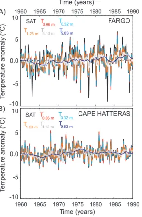
subsurface. Figure 1c shows NH land SAT averages in FOR 2 in comparison with temperature at the five soil model levels. Clearly, the highest frequencies have been filtered out and show considerable differences that will be discussed later in the text; at the lowest frequencies however subsurface temperatures and SAT share virtually

(14)

CPD

EGU

the same evolution (Gonz ´alez-Rouco et al., 2003b). Figure 1d illustrates differences between SAT and GST (represented byT_−0.06m) over the NH.T_−0.06m is on average 1.3 K warmer than SAT, most of this offset resulting from the contribution of thermally isolated areas caused by snow cover. Higher and mid-latitudes in North America and Eurasia present warmerT_{−0.06 m} than SAT related to snow insulation. Other regions of

5

the NH like Northern Africa (southern North America and southeastern Asia present warmer (colder) subsurface temperatures resulting from the availability of soil moisture and the balance of radiative and turbulent fluxes at the surface. These issues will be further discussed in Sect.3.

2.2 Geothermal models

10

Climate reconstruction of GST histories assumes that surface temperature variations propagate into the subsurface following the one dimensional time-dependent heat con-duction equation (Carslaw and Jaeger,1959):

δT δt = κ

δ2T δz2

where_{κ is the thermal diffusivity, which we can assume constant for the typical range}

15

of depths of interest for this work,z is the depth, and T is the temperature. In the

ab-sence of transient non-climatic disturbances at the ground surface or systematic per-turbations that violate the one-dimensional heat transfer assumption (heat production, topography, ground water flow,variations in thermal properties, etc.) the temperature at depth z is given, at any time, by the combination of the geothermal temperature

20

gradient and the temperature perturbation Tt(z) induced by the time varying surface

temperatures:

T (z) = T0+ q0R(z) + Tt(z), (1) whereq0 is the quasi steady state surface heat flow density and R(z) is the thermal

depth given by_R(z)=PN

i =1 (∆zi/λi) , λi being the thermal conductivity over the depth

(15)

CPD

Printer-friendly Version Interactive Discussion interval ∆zi.

Subsurface temperatures can be modeled using surface temperature as an upper boundary condition of an infinite half space. In turn, temperatures at the surface can be thought of as a series ofK step changes in temperature such that the subsurface

signatures from each step change are superimposed and the temperature perturbation

5

at depthz is given byMareschal and Beltrami(1992):

Tt(z) = K X k=1 Tk " erf c zj 2pκt_k ! − er f c z_j 2pκt_k−1 !# (2)

whereT_k is the ground surface temperature, each value representing an average over time (tk–tk−1), anderf c is the complementary error function.

This forward model can be used to derive grid point BTPs using simulated

sur-10

face temperature changes as boundary conditions; as suggested by Fig. 1c and in

Gonz ´alez-Rouco et al.(2006) the selection of SAT or temperatures at the various soil model levels is of no importance. The forward model is used herein to derive grid-point perturbation profiles 600 m deep using ECHO-g surface temperature changes as boundary conditions. At each 1 m depth interval a temperature anomaly is evaluated

15

from the contribution of surface temperature changes using the solution of the heat conduction equation in (2). Equation (2) is however sensitive to the reference temper-ature selected for the calculation of tempertemper-ature changes (T_k anomalies). This issue will be further discussed in Sects.3and4.

A singular value decomposition inversion model (SVD; Mareschal and Beltrami

20

(1992) is used to derive GST histories from grid-point BTPs. The thermal diffusivity value used for the forward and the inversion model applications was the same as in the ECHO-g GCM (0.75×10−6_m2_s−1_{). The model used for the inversion of each grid}

point BTP consists of a series of 20-yr step changes in GST history. The eigenvalue cutoff was set in different exercises between 0.025 and 0.3 to select the number of SVD

25

components (Mareschal and Beltrami,1992;Beltrami and Bourlon,2004). The singu-lar value cutoff is dependent in experimental practice on the model parameters, model

(16)

CPD

EGU

geometry and data noise level, and it varies among BTPs of the same region. Gener-ally, it is convenient to analyze BTPs with as similar geometry as possible to attempt to reduce the effects of different practical resolutions on the ensemble analysis.

3 Boreholes in the GCM surrogate reality

One strategy to test methods and assumptions in reconstruction approaches has been

5

to use GCM simulations as surrogates for the real climate evolution. Rather than rep-resenting the recent or past climate behavior, the simulations are meant to act as plau-sible climate realizations compatible with the external forcing imposed to the GCM, and complex enough to incorporate a variety of competing factors that contribute to the re-alism in the application of the target reconstruction technique (Mann and Rutherford,

10

2002;Zorita and Gonz ´alez-Rouco,2002;Zorita et al.,2003;Rutherford et al.,2003;von

Storch et al.,2004;Mann et al.,2005). Within the geothermal context, this approach has been used to explore potential caveats in the borehole approach to climate recon-struction through assessing various assumptions and methodological aspects. We will revisit some of this work along the following section and use it to further illustrate some

15

aspects relevant within the context of GST reconstructions from BTPs.

3.1 Discussing biasses on borehole temperature profiles

Mann and Schmidt (2003) and Schmidt and Mann (2004) used a 50 year long simula-tion of the GISS model to explore the effect of snow cover changes on seasonal SAT and GST coupling. They find a good summer link between both variables and report

20

that the winter SAT-GST relationship is disturbed by snow cover. They therefore argue that climate changes in winter SAT might not be as well translated into GST changes as in the warm season. If long term changes in snow cover have occurred during the last centuries these could have caused anomalous changes in GST relative to SAT by altering winter ground surface insulation by snow cover (see alsoStieglitz et al.,2003;

(17)

CPD

Zhang,2005). They argue that if a less intense hydrological cycle would have existed in the LIA due to a more frequent negative NAO phase (Shindell et al.,2001;Luterbacher

et al.,2001) this would have been consistent with a reduction in winter precipitation and snow cover. Such scenario would produce anomalous cooling of GST relative to SAT in the coldest phases of the LIA (e.g. LMM). Thus, in the event that climate changes over

5

the past few centuries would have been seasonally different there would be potential for a bias in GST reconstructions that could reflect colder temperatures during LIA than might actually have existed. They suggested that interpretations of past SAT trends from borehole-based GST reconstructions may therefore exaggerate LIA cooling and this could account for the differences of ca. 0.5 K found among existing reconstructions

10

(e.g.Mann et al.,1999;Huang et al.,2000).

The Mann and Schmidt (2003) arguments were debated byChapman et al. (2004) using the same GISS simulation and byBartlett et al.(2005) using observational snow cover, SAT and GST data. Chapman et al. (2004) argue that seasonal differences lead to seasonal offsets in GST and SAT averages and recommend that annual data

15

should be used in such an analysis. In doing so, they report good inter-annual tracking between GST and SAT through the examined 1951–1958 GISS simulated period. In a follow up study,Bartlett et al. (2005) argue that if the influence of snow on GST is not changing from year to year, such offset would be constant (e.g. Fig. 1d) and with no consequences for SAT and GST tracking. They agree that if snow cover is not

20

stationary its influence on the mean SAT-GST offset varies with time such that long term changes in snow cover may disrupt tracking between the two temperatures by introducing transient and persistent thermal signatures in the coupling. This possibility is examined by considering observations of snow cover changes in North America and their influence on the SAT-GST tracking. They quantified the changes in snow cover

25

onset and duration required to account for the approximately half a degree difference between borehole and multi-proxy climate reconstructions and report that it would be unlikely that changes in snow cover could account for this discrepancy. They find that in the 1970–2002 period, when winter SAT warming was the greatest, snow cover

(18)

CPD

EGU

inhibited 0.05 K/decade of seasonal warming from entering the ground, this being the result of a relatively stationary snow season under changing wintertime SAT.

These issues were also discussed using the millennial control and forced simula-tions with the ECHO-g model described in Sect.2.1 (Gonz ´alez-Rouco et al.,2003b,

2006) by assessing the relationship between NH SAT and GST at low frequencies. All

5

model simulations showed differences in both variables at high (seasonal and interan-nual to decadal) frequencies but demonstrated strong coupling between air and ground temperatures at low frequencies essentially as shown in Fig. 1c. This suggested that, within the limits of the reality simulated by the model, changes in surface conditions that perturb ground-air coupling like snow cover or sensible and latent heat fluxes are

10

not strong enough to decouple NH SAT and GST at long time-scales.

Figures 2 to 4 allow a perspective on the spatial variability of SAT-GST in relation to surface processes like snow and soil moisture changes. Figure 2a shows the average spatial distribution of snow depth in the FOR 2 simulation. The mid- to northern- latitude areas of GST insulation due to snow cover and their correspondence with the negative

15

SAT-GST offsets (Fig. 1d) are apparent. Figure 2b shows the correlation between an-nual snow depth changes and differences in anan-nual SAT and GST (SAT minus GST at 0.06 m depth,T_{−0.06 m}) in the same simulation. Air-ground temperature differences are related with changes in snow depth at inter-annual timescales and broadly dominate in the extra-tropical regions, thus supporting the influence of snow cover at annual and

20

longer time scales: negative correlations indicate increases (decreases) in snow depth associated with larger (smaller) SAT-GST negative offsets. There is general agreement with the finding byBartlett et al.(2005) that snow influence on the SAT-GST difference is greatest north of 45◦ _{in North America. Figure 2c and d shows linear trends in}

sim-ulated snow depth in an extended winter (DJFMA) season for the periods 1700–1990

25

and 1900 to 1990 AD. Values are realistic in comparison to observations (Brown and

Goodison,1996;Frei et al., 1999;Brown,2000;Brown et al.,2003) and interestingly they show increases (decreases) in snow depth over the northern (middle) latitudes since the simulated LIA to the end of the 20th century.

(19)

CPD

Printer-friendly Version Interactive Discussion Figure 3 allows the discussion to be extended to the possible influence of soil

mois-ture on air-ground temperamois-ture differences. The literamois-ture reports interesting changes in soil water content through the 20th century (e.g.Robock et al.,2000;Li et al.,2007;

Sheffield and Wood,2007) and, as in the case of snow depth/cover variations, these have the potential to change the ground temperature response by changing surface

5

latent heat fluxes and the heat capacity of the ground (Hu and Feng,2005;Kueppers

et al.,2007;Taylor et al.,2007). The average distribution of wetness (Fig. 3a) depicts areas of larger water content over Europe, the western Siberian plains, Southeastern Asia and the tropical areas of America and eastern North America. Correlations be-tween annual soil moisture and SAT-GST differences (Fig. 3b) illustrate the importance

10

of soil moisture changes on air-ground temperature coupling in the lower sub-tropical and tropical regions complementary to that of snow depth changes in the northern half of the NH (Fig. 2b). Soil moisture changes show opposite sense to those in absolute temperature differences at the surface, i.e., increases (decreases) in soil moisture tend to reduce (increase) the thermal difference between SAT and GST. In the areas of

pos-15

itive (negative) SAT-GST offset in Fig. 1d like eastern USA and eastern Asia (northern Africa and western USA) this translates into negative (positive) correlations in Fig. 3b. Such relation suggests that soil moisture could also be a factor in producing long term changes in ground-surface coupling and thus a bias in borehole temperatures. Fig. 3c and d show linear regression coefficients for the period 1700 to 1990 and 1900 to

20

1990 AD in annual soil moisture as simulated in FOR 2. These values are in the range of observed estimations for the second half of the 20th century (e.g. Robock et al.,

2000;Li et al.,2007). The simulated changes indicate for instance increases of soil moisture in northern Europe and decreases in mid-latitudes like the Mediterranean. These changes, as well as those shown above in snow depth would be consistent with

25

a northward shift of the hydrological cycle, thus, also compatible with a transition to a more zonal circulation (positive phase of the NAO) in the North Atlantic as hypothesized byMann and Schmidt(2003). In fact, FOR 1 and FOR 2 show long term transitions to a more zonal circulation from the LIA to the end of the simulations (e.g. Zorita et al.,

(20)

CPD

EGU 2005).

Figures 2 and 3 present a geographically complementary view of the domains of relevance of snow depth and soil moisture for air-ground coupling as well as a non stationary view of long term changes in both variables. However, snow cover and soil wetness changes are not the only two factors with potential to disrupt the

SAT-5

GST relation. Other factors introducing long term changes in soil radiative insulation and surface turbulent and radiative fluxes (e.g., vegetation or land use changes) can potentially bias GST respect to SAT variations. Examples are vegetation and land use changes. These type of variations are not included in the simulations and could potentially affect GST at long time scales (Bonan et al.,1992;Lewis and Wang,1998;

10

Bauer et al.,2003;Nitoiu and Beltrami,2005;Davin et al.,2007;Xu et al.,2007) and thus constitute issues which deserve attention in the future.

Long-term trends in SAT-GST differences during the simulated 20th century, (Fig. 4) show positive values indicating increases of SAT relative to GST over mid-latitudes and GST warming relative to SAT (negative trends) at northern latitudes. There are

15

no trends simulated in the areas of sensitivity of SAT-GST to soil moisture (Fig. 3b), thus the response suggests a relation with snow depth changes. Actually, there is regional agreement in broad spatial features in Figs. 2d and 4d like increasing snow depth (increasing the SAT-GST offset) over northern Eurasia and North America and decreasing snow depth (decreasing the SAT-GST negative offset) over the mid latitudes

20

and eastern Russia. Rather than long-term continuous changes, these linear trends arise in the simulations due to multi decadal changes along the second half of the 20th century. Figure 4c shows an example of SAT, GST and snow depth evolution at two characteristic points. The larger decreases (increases) in snow depth in the last decades in P 1 (P 2) lead to relative GST cooling (warming) with respect to SAT

25

changes due to increased exposure (insulation) to winter surface fluxes. The largest departures between SAT and GST anomalies go along with the largest changes in snow depth. While in P1 GST would under-estimate changes in SAT, in P 2 the contrary would happen.

(21)

CPD

Printer-friendly Version Interactive Discussion Therefore, Fig. 4 shows that large changes in snow depth/cover can modify the

SAT-GST relationship. The changes simulated by the model are reminiscent of those found in observations (e.g.Brown,2000) in as much as they reflect larger changes of snow cover for some regions along the last decades of the 20th century. Such decadal trends should have little influence on the estimation of multi-century trends that are imprinted

5

on borehole BTPs to depths of several hundred meters. Thus, as suggested byPollack

and Smerdon (2004), it is not easy to make a case for a systematic bias in subsurface temperatures due to these processes. In the surrogate reality of the model simulations, in spite of the changes in all variables represented by Figs. 2 to 4, there seems to be a negligible impact in the reconstruction of NH GST histories from simulated BTPs

10

(Gonz ´alez-Rouco et al.,2006).

It is worth noting that previous discussions or in methodological replications (e.g.

Gonz ´alez-Rouco et al.,2006) do not demonstrate that the borehole approach to cli-mate reconstruction is correct. The arguments rather lean on a null hypothesis that the methodology is actually competent in its purpose and the evidence either reveals

15

itself consistent with this statement or rejects it if results point in the opposite direction. Also, in this line of argumentation, it is not of relevance whether the model simulations reproduce the exact real past climate trajectories of the involved variables. Though desirable, most likely this will not be the case since the evolution of these variables will be largely subjected to internal, non-forced, climate variability and due to

limita-20

tions in model resolution and parametrizations (von Storch,1995;Raisanen,2007) to reproduce detailed aspects of snow depth and soil moisture dynamics (Brown,2000;

D ´ery and Wood, 2006; Robock and Li,2006; Li et al., 2007). The relevant issue in this approach, however, is whether the magnitude and spatial variability of simulated changes are realistic enough to assess whether changes in SAT-GST coupling within

25

the simulated reality would produce long-term biases in BTPs. In the case discussed herein, the model simulations do not show evidence to distrust the skill of the method in retrieving hemispheric estimates of past temperature changes. At the regional scales, however, the weight of trends in snow depth or other surface perturbations might be

(22)

CPD

EGU

larger and not lead to an overall balance as at hemispheric scales; an example ad-dressing regional scales will be shown in Sect.3.2.

3.2 Other methodological aspects

Beyond the questions raised above concerning SAT-GST coupling,Mann et al.(2003) further address various issues concerning observational and methodological aspects

5

that could account for the differences between borehole-based and other proxy-based climate reconstructions. Two major problems were discussed: (i) the influence of spa-tial aggregation and gridding of GST reconstructions from BTPs and of latitudinal area weighting to produce a NH temperature reconstruction; (ii) the apparent failure in GST reconstructions to reproduce a spatial structure of changes comparable to that of SAT

10

throughout the instrumental period. Mann et al. (2003) developed a NH temperature reconstruction for the last five centuries using theHuang et al.(2000) set of inverted NH BTPs in an optimal signal detection approach which was more in agreement with pre-vious multi-proxy reconstructions (Mann et al.,1999). These results were criticized by

Pollack and Smerdon(2004) who examined the impact of aggregation and area

weight-15

ing for various grid resolutions on the spatial consistency of GST and SAT trends. They concluded that low occupancy cells obscured the relation between SAT and GST and demonstrated the existence of spatial consistency in both sets of variables. In a re-vision of their initial workRutherford and Mann(2004) would later agree that gridding and area weighting do not resolve the differences between borehole and other proxy

20

reconstructions.

In addition to gridding and area-weighting, other possible methodological and obser-vational aspects that may degrade borehole reconstructions as representative indica-tors of SAT changes were discussed byMann et al.(2003) andPollack and Smerdon

(2004). Two of these are borehole site geography and logging dates. Both of this

25

issues can produce unclear biases in the datasets that could affect GST reconstruc-tions. The geographical distribution of boreholes is centered mostly in mid-latitudes and this could introduce a climatological bias in GST reconstructions. As for logging

(23)

CPD

Printer-friendly Version Interactive Discussion dates, the borehole data set (Huang and Pollack,1998) was compiled since the 1960’s

and different regions display some heterogeneity in logging dates (see Fig. 5c). This can produce biases by under-representing trends in regions where BTPs were logged earlier. While a geographical bias would potentially exaggerate warming by misrepre-senting low latitude regions and oceans that would warm less, the bias in the logging

5

dates would presumably under-represent warming by excluding the later 20th century decadal warming in regions where BTPs were logged earlier (Pollack and Smerdon,

2004).

The potential bias in the BTP geographical distribution was explored in the ECHO-g model simulations (Gonz ´alez-Rouco et al.,2006) by comparing the model response

10

using the whole array of model grid-points and a decimated mask overlapping with ar-eas where actual BTPs are available. Both spatial samples lead to virtually identical results, thus supporting the present distribution of BTPs as a viable sample for esti-mating terrestrial SAT variations. Gonz ´alez-Rouco et al. (2006) further illustrated the potential of the borehole methodology to produce GST reconstructions using a forward

15

model (see Sect. 2.2) to simulate synthetic BTPs within the model world and subse-quently inverting and averaging them to produce a hemispheric GST reconstruction that could be compared to the model simulated surface temperature.

This approach will be revisited in the remaining part of this section to illustrate how the method can be used to address the potential influence of logging dates and BTP

20

depth on borehole climate reconstructions. We will focus on North America as the example case where both variables show considerable spatial variability as depicted Fig. 5.

The original model grid (gray dots in Fig. 5a) was decimated to retain a subset of grid-points that were closer to the observational borehole network (red and green in

25

Fig. 5b, respectively).

BTPs were simulated at each location using GST anomalies at the deepest (−9.84 m) soil model level. Anomalies were calculated with respect to the full period of simulation and diffused downwards into the ground using Eq. (2) as described in

(24)

CPD

EGU

Sect. 2.2. This was done for the full model grid and for the subset of selected grid-points.

These simulated profiles represent a perfect world in terms of temperature perturba-tion profiles for which the SAT is known. These profiles can be inverted in order to test the potential of inversion models to retrieve GST histories in a process that mimics the

5

borehole approach to climate reconstruction. Additionally, the profiles can be further degraded making them more similar to real borehole temperature vs. depth anomalies and test the effect of degrading factors on the final reconstructions. Thus, the smaller grid-point subset was further deteriorated to incorporate a more realistic representation of possible biases related to logging dates and borehole depth.

10

The distribution of logging dates in the borehole dataset is spread over the last 40 to 50 years (Fig. 5c); overall the early measurements where made in USA and the more recent logs are distributed mostly over Canada. The potential impacts of this different distribution have been discussed in the previous section. This geographical spread is replicated within the model world over an equivalent range of 40 years (Fig. 5d),

15

ending in 1990 AD in order to accommodate the length of the model simulations. Model grid point series were trimmed according to this distribution before diffusing them into the ground. In this way, the simulated BTPs mimic within the model world different measurement moments. For the control simulation these dates are arbitrary since there is no correspondence to real years and were assigned in such a way to reproduce an

20

equivalent loss of data at the end of the simulation as it was done for the forced runs. A further degradation step consisted of shortening the simulated BTPs according to the real depth distribution shown in Fig. 5e and replicated in Fig. 5f. Though this distribution ranges over a depth of 1000 m, in practical terms only changes on the first ca. 400 m (see Fig. 6a) can have some effect, since bellow this depth the simulated

25

perturbation profiles virtually converge to zero. This approach attempts to address the impact of loosing part of the climatic history in some areas where boreholes are shallower.

(25)

CPD

Printer-friendly Version Interactive Discussion set of profiles (light shading) is highlighted in comparison to the smaller subset (dark

shading) decimated and corrupted by date and depth irregularities. The forced simula-tions present a tendency to larger warming in the top ca. 150 m representing the trends from the LIA to present. Bellow this depth, between ca. 300 m and 200 m some cooling is evident that relates to the transition from the simulated MWP to the LIA. Also, in

com-5

parison to the control run, the depth of warming onset is deeper in the forced than in the model simulations. In the control BTPs this shallower warming can be attributed to trends caused by internal variability at the end of the simulation (see CTRL in Fig. 1b). The simulated BTPs were inverted using SVD (Mareschal and Beltrami,1992) to obtain local GST histories and the mean was area-weighted over the whole domain. For each

10

local GST history, prior to the obtention of the spatial average, temperatures were kept constant since the logging date (Fig. 5d ) until 1990 AD in order to mimic published ex-ercises (e.g.Harris and Chapman,2001). This is a rather conservative scenario since in the real world applications there is availability of instrumental or reanalysis data that can be used to fill the gap after the logging date in a more accurate fashion. The cutoff

15

level used for the SVD-eigenvalues in this exercise was 0.025.

Figure 6b compares the low frequency evolution of North American SAT in each of the simulations and the latitude-average of the inverted GST histories, both for the complete grid (solid lines) and the perturbed subset (dashed lines); differences be-tween both GST inversions are highlighted.

20

The three GST histories successfully recover the low-frequency changes in North American SAT. The broad differences between the control and forced simulations are recovered, including the different level of MWP warming in FOR 1 and FOR 2. The differences between the full grid-point net and the perturbed subset are negligible in the context of the low frequency variability reproduced by the inverted histories. Thus,

25

Fig. 6b lends support for the borehole reconstruction approach in recovering low fre-quency changes of past temperature and suggests that the potential effects of vari-ability in logging dates and depths as simulated here are minor and will hardly explain offsets between borehole based and other proxy reconstructions.

(26)

CPD

EGU

Nevertheless, this exercise rests on some assumptions that are worth discussing. Since this approach only simulates temperature perturbation profiles, i.e. the Tt(z)

terms in Eq. (1), all the potential problems related to the separation of the climate transient, T_t(z), from the geothermal gradient in Eq. (1), T0+q0R(z), are overlooked.

Additionally, there are at least two relevant issues when separating the geothermal and

5

climatological information in BTPs: the actual depth of the profiles and the existence of noise.

The treatment given to borehole depth in Figs. 5 and 6 addresses the fact that shal-lower boreholes miss a part of the climate history recorded deeper into the ground but skips the problems of discriminating the geothermal from the climatological signal

10

in shallower boreholes which have not fully met the geothermal equilibrium gradient. Thus, the previous results assume that there is a perfect separation between both types of signals and addresses only potential problems related to the subsequent processing of perturbation profiles.

Borehole noise is another issue that further complicates both the inversion of

pertur-15

bation profiles and the discrimination between the geothermal background and the cli-mate transient. The latter problem could be easily addressed by adding some realistic noise to the temperature profiles and continuing with the other steps of the methodol-ogy. Therefore, an additional improvement of the approach that can be considered in future work is the simulation of a random and realistic spatial distribution of

geother-20

mal gradient values and noise that will allow for a more realistic reproduction of all the steps of the procedure. However, it is not clear that the inclusion of these features will lead to large biases in the recovered GST histories since errors in separating the terms in Eq. (1) at each BTP should randomly distribute contributing to produce under- and over- estimations of surface temperature.

25

The impact of noise in perturbation profiles is in practice overcome by considering smoother solutions to the heat diffusion equation. In the case of the SVD inversion ap-proach used herein this implies the use of larger eigenvalue cutoff levels, thus retaining less information from the measurements. This avoids unstable solutions produced by

(27)

CPD

Printer-friendly Version Interactive Discussion over-weighting errors in the eigen modes (see discussion inBeltrami and Mareschal,

1995;Beltrami and Bourlon,2004). The effects of this can be observed in Fig. 6c where various GST histories corresponding to cutoff levels between 0.025 and 0.3 are shown for the case of the FOR 1 simulation. The 0.025 value is rather low and appropriate for noise-free profiles whereas values between 0.1 and 0.3 are typical of real profiles with

5

the presence of noise (Beltrami and Bourlon,2004).

The provided solutions show a progressive decrease of the differences between the original complete set of GST grid-point BTPs and the date and depth perturbed subset. Also a progressive loss of skill in depicting the warming from the LIA to the MWP is observed in addition to less cooling from the simulated 20th century to the LIA.

10

Interestingly, this behavior suggests that a more realistic replication of the borehole method leads to under- rather than over- estimation of past climate variability and, in particular, LIA cooling.

A last comment in this discussion concerns the assumption implicit in calculating temperature anomalies with respect to the full period of simulation before producing

15

BTPs. This apparently innocuous step is arbitrary and not free from quite strong as-sumptions since the selection of a reference period, and thus a mean temperature reference value for the calculation of anomalies produces important changes in the simulation of BTPs. However, the selection of a particular reference is irrelevant if the analysis rests on taking for granted that a perfect discrimination between the

geother-20

mal gradient and the climate transient is possible. Under this assumption, the analysis starts by adopting the simulated perturbation BTPs as valid and addressing all sub-sequent aspects of the methodology. Decisions concerning the selection of a mean temperature reference level to calculate anomalies bear more importance in the com-parison of observational and simulated BTPs. Therefore, this will be further discussed

25

(28)

CPD

EGU

4 Simulations and observations

Section3was focused on some questions that can be addressed by using models as a surrogate for reality. However it is also pertinent to analyze the degree of realism of GCMs in reproducing some aspects of reality. In the geothermal context there are at least two directions along which such questions can be posed: 1) the agreement

5

between GCM simulations and observed BTPs; 2) the level of fidelity with which GCMs can recreate the details of the air-ground temperature coupling at local scales. The first point targets the comparison of model simulations and borehole paleoclimatic recon-structions or BTPs. The second question attempts to address whether the degree of realism of the simulated land surface processes is adequate both in the paleoclimatic

10

and in the future climate change context.

4.1 Simulated and observed borehole temperature profiles

Reliable projections of future change require that climate models prove effective in simulating past changes in broad agreement with evidence provided by climate re-constructions. Advances in the convergence between simulation and reconstruction

15

approaches will require reducing various types of uncertainties on both sides (Jansen

et al., 2007; Hegerl et al., 2007b). Joint analysis of climate reconstructions, model simulations and estimated past external forcing can illustrate the level of agreement between model results and reconstructions (Jones and Mann,2004;Zorita et al.,2004;

Moberg et al.,2005), but also to try to constrain the range of climate sensitivity (Hegerl

20

et al.,2006) and to attribute past changes registered in millennial climate reconstruc-tions to particular external forcings (Crowley,2000;Bauer et al., 2003; Hegerl et al.,

2003).

In the context of borehole climate reconstructions, first steps have been taken in designing a means of comparison of the information provided by BTPs with model

25

simulations. Beltrami et al. (2006b) compared the output of the ECHO-g simulations presented herein with BTPs in four regions over Canada. For each region, annual

(29)

CPD

Printer-friendly Version Interactive Discussion averages of ECHO-g simulated SATs were used to construct the subsurface thermal

profiles as described in Sect.3.2. These were subsequently compared with average BTPs measured at each region. It was found that in all cases subsurface anomalies so calculated from the forced simulations were in better agreement with observed profiles than the synthetic profiles derived from the control simulation.

5

Stevens et al.(2008) arrived at the same conclusion in an extension of the analysis to the whole of North America in which alternative ways of comparing real and sim-ulated profiles are explored. Both studies target a broad evaluation of agreement or disagreement between observed BTPs and model simulations, and in their conclusions they qualitatively support the sensitivity of BTPs to external forcing and thus their

use-10

fulness for climate change assessment; however these works cannot be included in the context of climate attribution since the model simulations involved cannot discriminate among the influence of various natural and anthropogenic forcings.

Stevens et al.(2008) andBeltrami et al.(2006b) also highlighted a seemingly qual-itative agreement in the east-west arrangement of trend in the observed and in the

15

synthetic boreholes from the forced simulation over northern North America. Lower (larger) amplitude of warming has been reported for the western (central and eastern) parts of Canada (Majorowicz et al.,2002) and, in particular, changes from the western to the eastern side of the Cordillera have been noted (Wang et al.,1994;Pollack and

Huang,2000). Figure 7 provides a spatial perspective into the trends simulated by the

20

ECHO-g model for the period 1700 to 1990 AD. In spite of different internal non-forced variability in each simulation, both model integrations produce a remarkably similar pattern with smaller trends over western Canada and larger trends in the central and eastern territories. The large-scale temperature response in these model simulations is shown inZorita et al.(2005) and can be described as a land-ocean thermal contrast.

25

This pattern is superimposed to regional trends that are associated with changes in the intensity of the main modes of atmospheric circulation.

Over North America most of the main land and the regions usually covered by peren-nial snow the model simulates larger warming in the continent with diminishing