HAL Id: hal-01714121
https://hal.archives-ouvertes.fr/hal-01714121
Submitted on 22 Aug 2020
HAL is a multi-disciplinary open access
archive for the deposit and dissemination of
sci-entific research documents, whether they are
pub-lished or not. The documents may come from
teaching and research institutions in France or
abroad, or from public or private research centers.
L’archive ouverte pluridisciplinaire HAL, est
destinée au dépôt et à la diffusion de documents
scientifiques de niveau recherche, publiés ou non,
émanant des établissements d’enseignement et de
recherche français ou étrangers, des laboratoires
publics ou privés.
The optical properties of galaxies in the Ophiuchus
cluster
Florence Durret, Ken’Ichi Wakamatsu, Christophe Adami, Takahiro
Nagayama, J. Marissol Omega Muleka Mwewa Mwaba
To cite this version:
Florence Durret, Ken’Ichi Wakamatsu, Christophe Adami, Takahiro Nagayama, J. Marissol Omega
Muleka Mwewa Mwaba.
The optical properties of galaxies in the Ophiuchus cluster.
Astronomy
&
Astrophysics
https://doi.org/10.1051/0004-6361/201731371© ESO 2018
The optical properties of galaxies in the Ophiuchus cluster
?
F. Durret
1, K. Wakamatsu
2, C. Adami
3, T. Nagayama
4, and J. M. Omega Muleka Mwewa Mwaba
5,61Sorbonne Université, CNRS, UMR 7095, Institut d’Astrophysique de Paris, 98bis Bd Arago, 75014 Paris, France
e-mail: [email protected]
2Faculty of Engineering, Gifu University, 1–1 Yanagido, Gifu 501-1193, Japan
3LAM, OAMP, Pôle de l’Etoile Site Château-Gombert, 38 rue Frédéric Joliot–Curie, 13388 Marseille Cedex 13, France 4Department of Astrophysics, Kagoshima University, Nagoya, Japan
5Universidade Federal de Sergipe, Departamento de Física, Av. Marechal Rondon, S/N, 49000-000 São Cristóvão, SE, Brazil 6CAPES Foundation, Ministry of Education of Brazil, Brasilia â DF, 70.040-020, Brazil
Received 14 June 2017 / Accepted 24 January 2018
ABSTRACT
Context. Ophiuchus is one of the most massive clusters known, but due to its low Galactic latitude its optical properties remain poorly known.
Aims. We investigate the optical properties of Ophiuchus to obtain clues on the formation epoch of this cluster, and compare them to those of the Coma cluster, which is comparable in mass to Ophiuchus but much more dynamically disturbed.
Methods. Based on a deep image of the Ophiuchus cluster in the r0
band obtained at the Canada France Hawaii Telescope with the MegaCam camera, we have applied an iterative process to subtract the contribution of the numerous stars that, due to the low Galactic latitude of the cluster, pollute the image, and have obtained a photometric catalogue of 2818 galaxies fully complete at r0= 20.5 mag
and still 91% complete at r0= 21.5 mag. We use this catalogue to derive the cluster Galaxy Luminosity Function (GLF) for the overall
image and for a region (hereafter the “rectangle” region) covering exactly the same physical size as the region in which the GLF of the Coma cluster was previously studied. We then compute density maps based on an adaptive kernel technique, for different magnitude limits, and define three circular regions covering 0.08, 0.08, and 0.06 deg2, respectively, centred on the cluster (C), on northwest (NW)
of the cluster, and southeast (SE) of the cluster, in which we compute the GLFs.
Results. The GLF fits are much better when a Gaussian is added to the usual Schechter function, to account for the excess of very bright galaxies. Compared to Coma, Ophiuchus shows a strong excess of bright galaxies.
Conclusions. The properties of the two nearby very massive clusters Ophiuchus and Coma are quite comparable, though they seem
embedded in different large-scale environments. Our interpretation is that Ophiuchus was built up long ago, as confirmed by its relaxed state (see paper I) while Coma is still in the process of forming.
Key words. galaxies: clusters: individual: Ophiuchus – galaxies: luminosity function, mass function – galaxies: photometry
1. Introduction
The Ophiuchus cluster is one of the most massive nearby clus-ters, at a redshift of z= 0.0296. Since its discovery (Wakamatsu & Malkan 1981;Johnston et al. 1981), it has been studied in detail in X-rays (seeWerner et al. 2016and references therein), but due to its low Galactic latitude (b= 9.3◦) its optical properties are not well known. In a previous paper (Durret et al. 2015, hereafter paper I), we have shown that overall the cluster can be consid-ered as relaxed, composed of a main structure and a single, much smaller substructure, with a total mass of 1.1 × 10¹⁵ M
. We
present here our photometric catalogue of 2818 galaxies in the r0band, and discuss the galaxy luminosity function (GLF) in the
overall image, in a region (hereafter the “rectangle” region) cov-ering exactly the same physical size as the region in which the GLF of the Coma cluster was studied byAdami et al.(2007), and in three regions of the cluster.
In spite of numerous studies, GLFs do not seem to have prop-erties that can be predicted based on the simple knowledge of the cluster mass or structure (relaxed or not). GLFs are usually
?The photometric catalogue of Ophiuchus (full TableB.1)
is only available at the CDS via anonymous ftp to
cdsarc.u-strasbg.fr(130.79.128.5) or via
http://cdsarc.u-strasbg.fr/viz-bin/qcat?J/A+A/613/A20
fit by a Schechter function (Press & Schechter 1974) but devi-ations from this function are often observed, in particular in merging clusters, which often show an excess of very bright galaxies. At the other end of the GLF, the faint end slope α pro-vides information on the cluster formation and evolution (see e.g. Martinet et al. 2015). However, we note that α seems to vary from one cluster to another with no obvious dependence on the cluster properties. Deriving the GLF of Ophiuchus and comparing it to that of other massive nearby clusters such as Coma, which shows a much higher level of substructuring, could reveal interesting differences or similarities between two clusters of comparable mass, one relaxed and the other non-relaxed.
In a preliminary study based on an extensive redshift cat-alogue combining their own data with archive data from 6dF and NED, Wakamatsu et al. (2005) analysed the distribu-tion of 4717 galaxies with recession velocities in the range 500 < cz < 40 000 km s−1. They showed that Ophiuchus is suf-ficiently large and rich to be considered a supercluster, which they call the Ophiuchus supercluster.Wakamatsu et al. (2005) also detected a wall structure 65 Mpc in length between Ophi-uchus and a zone from where the Hercules supercluster extends to the north. They noted that this wall runs close to north-south and crosses the Great Wall perpendicularly at the Her-cules supercluster. Another wall could be a continuation of
A&A 613, A20 (2018)
the Ophiuchus-Hercules wall across and beyond the Galactic plane. They also found a strong deficiency of galaxies with velocities cz < 4000 km s−1, thus extending the Local Void
beyond the limit determined byTully & Fisher(1987). So Ophi-uchus seems to show particularities at large scales, and this will be investigated in a companion paper (Wakamatsu et al. in prep.). As in paper I, we adopt the following quantities: cluster cen-tre RA = 258.1155◦, Dec = −23.3698◦ (coordinates of the cD
galaxy), a scale of 0.585 kpc/arcsec, and a distance modulus of 35.54.
2. The photometric galaxy catalogue
The study presented here is based on the full exploitation of the CFHT/MegaCam image that we obtained in the r0 band.
Magnitudes have been measured in the AB photometric sys-tem. At the redshift of Ophiuchus, the 1 × 1 deg2 MegaCam
field corresponds to a region of about 2.1 × 2.1 Mpc2. This cov-ers part of the cluster (for which r200 = 2.1 Mpc (see Table 2
in Paper I). As explained in Paper I for our pilot survey in a small area (10 × 9.5 arcmin2) centred on the cD galaxy, an
automated galaxy survey did not work properly for the Ophi-uchus cluster due to the high density of foreground stars. Instead, we made our galaxy survey based on the visual inspection of star-subtracted images, which are created from original ones with a PSF-deblending algorithm. After this process, galax-ies are fairly easily found. To make the survey as uniform as possible for the present large sky area (about 1 deg2), we set
the limiting magnitude about 1.5 mag brighter than the previ-ous pilot survey and iterated the survey four times, going to fainter magnitudes step by step. This work was done by one of us (K.W.) and his research assistant. Finally we picked 2818 galaxies, including 227 galaxies that were in the pilot survey of Paper I.
We now produce a full r0band magnitude catalogue for the
entire 1 deg2region covered by MegaCam, including the galaxies
from Paper I, and containing 2818 galaxies. Since our observa-tions were made in 2010, the r0band filter mounted on MegaCam
was a first generation filter. Magnitudes in this filter (in the AB system) are very close to the SDSS magnitudes: as indicated in the MegaCam pages1, the relation between the MegaCam and SDSS r band magnitudes is:
rMegaCam− rSDSS= −0.024 (gSDSS− rSDSS). (1)
For elliptical galaxies at redshift z = 0 (the galaxy type expected to be dominant in Ophiuchus), Fukugita et al.
(1995) give gSDSS − rSDSS = 0.77, in which case rMegaCam
= rSDSS − 0.013. For other types of galaxies, the difference
between rMegaCam and rSDSS will be even smaller. In view of
the error bars on magnitudes (see Table A.1) and of the large extinction correction that must be applied (see below), we here-after neglect the difference between rMegaCam and rSDSS. All the
galaxies were treated as described in Paper I (iterative star sub-traction) and subimages were extracted around each galaxy after the stars were eliminated. The varying extinction in the field results in a different sensitivity to galaxy intrinsic surface bright-ness with position. This will impact photometric methods based on a thresholding in surface brightness for object measurements, such as isophotal magnitudes or Kron magnitudes. For this rea-son, we have used SExtractor MAG_MODEL magnitudes based on a profile fit rather than the classical MAG_AUTO. The PSF
1 http://www.cadc-ccda.hia-iha.nrc-cnrc.gc.ca/en/
megapipe/docs/filt.html
Fig. 1. Observed magnitude histogram in the r0
band for the galaxies included in the 1 deg2region covered by our MegaCam image (before
applying any extinction correction). The 2499 galaxies of the prelimi-nary survey are shown in red and the 319 galaxies of our second survey are shown in blue.
was measured with PSFEx2, and a Sersic profile convolved with
this PSF was fit to each galaxy using SExtractor (Bertin & Arnouts 1996), giving MAG_MODEL magnitudes.
To illustrate the depth of the photometric catalogue, we show in Fig.1the corresponding apparent magnitude histogram. Nearly half of the galaxies in the three faintest bins in Fig.1are galaxies found in the pilot survey given in Paper I, implying that the present galaxy survey in the large area is shallower than the pilot survey.
To check the completeness of our preliminary galaxy sur-vey containing 2499 galaxies, we marked on the star-subtracted images the detected galaxies with 20.0 < r0< 22.0 with
differ-ent symbols in 0.5 mag intervals, and made the galaxy survey again for the full 1 deg2area. We did our best not to miss them
during the survey process by changing the contrast and/or bright-ness level on the ds9 image viewer. Out of these newly detected galaxies (∼450), photometric measurements were made for 319 galaxies among the brightest. The present catalog therefore comprises 2499 + 319 = 2818 objects.
The magnitudes of the five brightest galaxies among these newly detected objects are 19.44, 19.85, 19.90, 20.13, and 20.33 mag, respectively. Also follow 12, 14, 13, and 24 galaxies, in the successive magnitude ranges from 20.5 to 21.5 with a step of 0.25 mag. One quarter of the 319 galaxies are brighter than 21.5 mag, while three quarters are fainter than this magnitude (Fig.1). Based on these counts, we estimate that the catalogue is fully complete down to 20.5 mag, and almost complete (98.5%) down to 20.75 mag. However, when the sensitivity variations among the 25 CCD detectors of MegaCam as well as the exis-tence of faint diffuse nebular emission in this area of the Galactic plane are taken into account, there may still exist missed galax-ies brighter than 20.5 mag, for example, diffuse galaxgalax-ies of low surface brightness or compact galaxies of small (∼2.5 arcsec) angular diameter. The former may be missed due to irregulari-ties of the sky background, while the latter can be hidden by the
2 http://www.astromatic.net/
Fig. 2. Galactic extinction map in the Ophiuchus region. The white square shows the MegaCam field, and the three circles are those defined in Sect.3.3. Extinction increases from blue to red and to yellow. The MegaCam field is oriented with North to the top and east to the left, and the extinction map is slightly tilted.
Fig. 3.Histogram of the Galactic extinction in the r0
band for the 2818 galaxies of our photometric catalogue.
spiders of bright foreground stars or by multiply blended stars. We finally estimate that the present catalogue is really complete down to r0 = 20.25 ± 0.25 mag. The completeness in absolute
magnitude is discussed in Sect.3.1
We note that the shortage of galaxies fainter than Mr0 = −20
in zone C is real (see Sect.3.4), and is not due to the incomplete-ness of our survey in the core region.
At such a low Galactic latitude, Galactic extinction is obvi-ously large. We first adopted the value of 1.357 mag given by NED for the SDSS r band. We then decided to go one step further and look in more detail at the Galactic dust extinc-tion map by Schlegel et al.(1998) with newer estimates from
Schlafly & Finkbeiner(2011)3. The map contains the values of the colour excess E(B − V) with a pixel size of 1.5 arcmin. We converted it to an extinction map Ar in the r0 band, by
multi-plying it by R= 2.285 (value taken fromSchlafly & Finkbeiner 2011, Table 6), that is, Ar= R × E(B − V).
The extinction varies quite strongly in the region covered by our image: between 1.025 and 2.02, as illustrated in Fig.2. When computing GLFs in Sect.3we therefore applied either the con-stant extinction of 1.357 mag or the individual extinction for each galaxy.
The heavy galactic extinction for the Ophiuchus cluster causes a reduction of the apparent angular size of each galaxy, which could require further extinction correction. However, this correction amounts to 0.15 mag at most, and it depends in a com-plicated way on the adopted colour band and morphological type of each galaxy (Cameron 1990), so we decided not to apply it.
The final photometric catalogue of 2818 galaxies will be made available in ViZieR at the CDS4. For each galaxy, it
con-tains the following information: RA, Dec, measured r0 band magnitude with no extinction correction, magnitude corrected for a constant value of 1.357 mag, magnitude corrected for the individual extinction of each galaxy, major and minor axes (a and b), position angle (PA) of the major axis, and error on the PA. The values of a and b are the angular sizes of the semi-major and -minor axes which are computed from the 1σ values of the half-axes given by SExtractor, multiplied by a factor 4.0 to fully enclose the galaxies (as advised in the SExtractor manual). The typical errors on the magnitudes, estimated from a subsample of more than 40 galaxies measured twice (in adjacent fields), are given in TableA.1. The first ten lines of the catalogue are shown in AppendixB.
3. The galaxy luminosity function of the Ophiuchus cluster
3.1. The global galaxy luminosity function
To compute the GLF of the Ophiuchus cluster, it is necessary to statistically subtract the background contribution. Our orig-inal galaxy counts in the CFHT/MegaCam field are shown in Fig.1. We first corrected them for a constant extinction of 1.357. Background counts were taken fromYasuda et al.(2001), who estimated field galaxy counts from the SDSS at relatively bright magnitudes. They show galaxy counts in the r0 magnitude in
their Fig. 4. Since these counts are taken in the same filter as our data, in bins of 0.5 mag, and normalized to 1 deg2, we
can subtract them from our counts in a straightforward way to obtain the GLF (after normalizing our data to the area covered by our image: 0.9882 deg2). As a check to the Yasuda et al.
counts, we also plotted on the same figure the VVDS counts by
McCracken et al.(2003), that we cannot use here since they start at a magnitude of 18. We can see in Fig.4 that the two sets of background counts match well. We converted apparent to abso-lute magnitudes by applying the distance modulus of 35.54, and thus obtained Fig.4. In view of the small redshift of the cluster, we applied no k-correction.
However, we can see in Fig. 4that the Yasuda background counts become larger than our galaxy counts for Mr0 ∼ −16.3,
corresponding to r0 ∼ 19.2, a value which is more than one magnitude brighter than our completeness limit (r0 = 20.25).
This leads us to think that due to cosmic variance the Yasuda
3 http://irsa.ipac.caltech.edu/applications/DUST/
A&A 613, A20 (2018)
Fig. 4.Galaxy counts in the r0
band converted to absolute magnitude (see text). The red histogram shows the 2818 galaxies from our cata-logue and the cyan histogram those with spectroscopic redshifts in the cluster range, both corrected for a constant galactic extinction of 1.357 as explained in Sect.2. The green histogram shows the 2818 galaxies from our catalogue corrected for their individual galactic extinction. The blue and black lines show the field galaxy counts computed byYasuda
et al.(2001), andMcCracken et al.(2003) respectively. The blue
dot-ted and dashed lines show the Yasuda background counts multiplied by 0.85 and 0.70, respectively (see Sect.3.1).
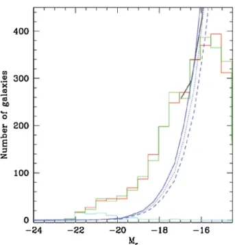
Fig. 5.Galaxy luminosity function of the Ophiuchus cluster in the entire
MegaCam field. The black line and points are the data, the green curve is the Gaussian component, the blue curve is the Schechter function, and the red curve is the total of the two components. Top: constant galac-tic extinction correction of 1.357, bottom: individual galacgalac-tic extinction correction. Left: subtraction of Yasuda background counts, and right: subtraction of Yasuda background counts multiplied by f = 0.7 (see Sect.3.1).
counts are an overestimate of the background counts in the direc-tion of Ophiuchus. Our extensive redshift catalogue in this area (Wakamatsu et al. in prep., see also Wakamatsu et al. 2005) indeed shows that besides the foreground (cz < 6000 km s−1)
local void, there is also a large background void behind the Ophiuchus cluster, up to cz ∼ 16 000 km s−1. Therefore the
back-ground contamination for the cluster should mostly come from the background galaxies with velocities cz > 16 000 km s−1.
To examine how Yasuda’s background data are modified by this cosmic variance, we carried out numerical simulations by changing the values of various parameters of the Schechter function, such as M∗, α, and the faintest magnitude cutoff, as well as the integration limit of the depth (distance modu-lus (m − M) < 40.5). The results show that these voids affect effectively the GLF parameters for r0 > 17, or Mr0 > −17.5 in
absolute magnitude. However, we cannot obtain a unique solu-tion, and all we can say is that the Yasuda background counts should be multiplied by a factor f = 0.85 ± 0.15. We therefore fit the various GLFs with the values of f that bracket this interval:
f = 1.0 and f = 0.70, noted, respectively, f and f0hereafter.
Since our galaxy counts show an excess of bright galaxies, we accounted for this excess with a Gaussian function G(M) (the values of the reduced χ2are indeed much lower when a Gaussian
is included), and we fit the GLFs with a global function:
GLF(M)= S (M) + G(M). (2)
Here S (M) is the Schechter function defined in terms of the absolute magnitude M as:
S(M)= 0.4 ln 10 Φ∗yα+1e−y (3) with y= 100.4 (M∗−M), where Φ∗ is a normalisation factor, M∗ is the typical magnitude separating the bright and faint regimes of the GLF, and α is the faint end slope. G(M) is a Gaussian function to account for the bright part:
G(M)= A exp[(−4 ∗ ln(2) ∗ (M − Mc)2)/( f whm2)] (4)
where Mcis the central magnitude, f whm is the
full-width-at-half maximum and A is the amplitude for M= Mc.
We also tried to fit the GLFs with a global function including the factor f ≤ 1 by which the Yasuda background counts should be multiplied:
GLF(M)= S (M) + G(M) + f ∗ B(M). (5) However, the addition of a seventh free parameter made the solution quite uncertain: the reduced χ2 remained almost the same for all the values of f , and the f parameter space did not seem to be explored properly, so it was not possible to estimate f with this method. We therefore decided to fit all the GLFs with the sum of a Gaussian and a Schechter functions, multiplying the Yasuda counts by f and f0.
It should be noted that the large excess of bright galaxies in the GLFs is not affected by the ambiguity of the field galaxy correction, which is very small for bright galaxies.
We computed the GLF both for a constant (noted “ct.” in Table1) galactic extinction of 1.357 and for a galactic extinc-tion that is different for each galaxy (noted “var.” in Table1), as explained above. The results of the Gauss+Schechter fits are shown in Fig.5and the corresponding parameters are given in Table1. The reduced χ2 values of the fits are 0.81 and 0.72 for a constant and a variable extinction correction, respectively. The reduced χ2values are larger than 2.0 if no Gaussian component is included, therefore justifying our choice of a Gauss+Schechter fit to the GLFs.
We can see that the galaxy counts do not vary strongly with the method used to correct for galactic extinction (Fig. 4), as confirmed by the fact that the shapes and parameters of the GLF fits are quite similar in both cases, and agree within the error bars (Table1). Of course if we take f0= 0.7 the counts are higher, and the parameters of the fit change.
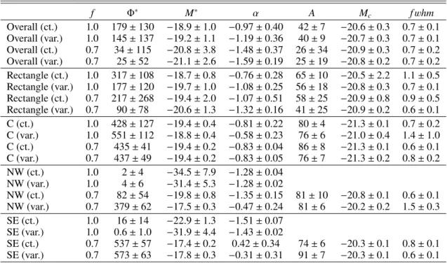
Table 1. Parameters of the GLF for the overall image, with magnitudes corrected for extinction with a constant value (ct.), or with their individual values (var.), as well as for the rectangular region with the same physical size as the GLF computed for the Coma cluster, and for the three circular regions C, NW and SE (see text).
f Φ∗ M∗ α A Mc fwhm Overall (ct.) 1.0 179 ± 130 −18.9 ± 1.0 −0.97 ± 0.40 42 ± 7 −20.6 ± 0.3 0.7 ± 0.1 Overall (var.) 1.0 145 ± 137 −19.2 ± 1.1 −1.19 ± 0.36 40 ± 9 −20.7 ± 0.3 0.7 ± 0.1 Overall (ct.) 0.7 34 ± 115 −20.8 ± 3.8 −1.48 ± 0.37 26 ± 34 −20.9 ± 0.3 0.7 ± 0.2 Overall (var.) 0.7 25 ± 52 −21.1 ± 2.6 −1.59 ± 0.19 25 ± 19 −20.8 ± 0.2 0.7 ± 0.2 Rectangle (ct.) 1.0 317 ± 108 −18.7 ± 0.8 −0.76 ± 0.28 65 ± 10 −20.5 ± 2.2 1.1 ± 0.5 Rectangle (var.) 1.0 177 ± 120 −19.7 ± 1.0 −1.08 ± 0.25 56 ± 18 −20.8 ± 0.3 0.7 ± 0.1 Rectangle (ct.) 0.7 217 ± 268 −19.4 ± 2.0 −1.07 ± 0.51 58 ± 25 −20.9 ± 0.8 0.9 ± 0.5 Rectangle (var.) 0.7 90 ± 78 −20.6 ± 1.3 −1.32 ± 0.16 41 ± 25 −20.9 ± 0.2 0.6 ± 0.1 C (ct.) 1.0 428 ± 127 −19.4 ± 0.4 −0.81 ± 0.22 80 ± 4 −21.3 ± 0.1 0.7 ± 0.2 C (var.) 1.0 551 ± 112 −18.8 ± 0.4 −0.58 ± 0.23 76 ± 6 −21.0 ± 0.4 1.4 ± 1.0 C (ct.) 0.7 435 ± 41 −19.4 ± 0.2 −0.83 ± 0.04 86 ± 8 −21.3 ± 0.1 0.6 ± 0.1 C (var.) 0.7 437 ± 49 −19.4 ± 0.2 −0.83 ± 0.05 76 ± 7 −21.3 ± 0.2 0.8 ± 0.2 NW (ct.) 1.0 2 ± 4 −34.5 ± 7.9 −1.28 ± 0.04 NW (var.) 1.0 4 ± 6 −31.4 ± 5.3 −1.28 ± 0.02 NW (ct.) 0.7 82 ± 54 −19.8 ± 0.8 −1.35 ± 0.15 81 ± 10 −20.8 ± 0.1 0.6 ± 0.1 NW (var.) 0.7 379 ± 62 −17.5 ± 0.3 −0.47 ± 0.24 81 ± 6 −20.2 ± 0.2 1.5 ± 0.3 SE (ct.) 1.0 16 ± 14 −22.9 ± 1.3 −1.51 ± 0.07 SE (var.) 1.0 0.6 ± 1.0 −31.9 ± 4.4 −1.43 ± 0.02 SE (ct.) 0.7 537 ± 57 −17.4 ± 0.2 0.42 ± 0.34 74 ± 6 −20.3 ± 0.1 0.8 ± 0.1 SE (var.) 0.7 573 ± 63 −17.8 ± 0.3 −0.31 ± 0.31 91 ± 7 −20.3 ± 0.1 0.6 ± 0.1
Notes. f is the factor by which the Yasuda background counts were multiplied to account for cosmic variance.
We note that the faintest bins in which we can compute the GLF are at absolute magnitudes of −17.5 and −16.5, for f = 1.0 and f0 = 0.7, respectively, brighter or comparable to the
com-pleteness limit of our photometric catalogue (−16.4) given in the previous section; therefore they can be considered as reliable.
The fits appear quite satisfactory in view of all the difficul-ties overcome to obtain a photometric catalogue. The Gaussian components are in both cases important at bright magnitudes. An excess at very bright magnitudes seems to be quite a general phenomenon, as already noted for example in Abell 223 (Durret et al. 2010), Abell 1758 (Durret et al. 2011) or Abell 3376 (Durret et al. 2013). But all these clusters were mergers, so we did not expect to find such a large Gaussian component in Ophiuchus, which is believed from previous studies to be quite relaxed. The faint end slope is moderate for f = 1.0 (α = −0.97 or −1.19, depending on the way the extinction is corrected), and steeper for f0= 0.7 (−1.48 to −1.59).
The latter steep values could be due to a non-negligible back-ground contamination at faint magnitudes. However we note that comparable values have already been observed in other clusters. For example, in the nearby massive cluster Coma,Adami et al.
(2007) found a faint end slope even steeper than −1.49 in the north part of Coma, which is a relatively quiescent region, and a flatter slope around −1.3 in the south half of Coma, which is experiencing infalls.
This led us to derive the GLF in a region having the same physical size as for Coma, to make the comparison of these two clusters more reliable. Our results are described in the following section.
3.2. The galaxy luminosity function in a physical region similar to our previous study of the Coma GLF
Adami et al.(2007) analysed the GLF of the Coma cluster in a region covering 40 arcmin in right ascension and 50 arcmin
Fig. 6. Galaxy luminosity function of the Ophiuchus cluster in the
“rectangle” region (covering the same physical size as for the Coma cluster; see text). Top: constant galactic extinction, bottom: individual galactic extinction correction. Left: subtraction of Yasuda background counts, and right: subtraction of Yasuda background counts multiplied by f = 0.7 (see Sect.3.1). See caption of Fig.5for colour coordination of lines and curves.
in declination. At the redshift of Coma, this corresponds to a zone of 1.1136 × 1.3920 Mpc2. Since the scale for Ophiuchus is 0.585 kpc arcsec−1, this size corresponds to a region of
0.5288 × 0.661 deg2, or a surface of 0.34954 deg2. We there-fore extracted from our photometric catalogue a zone defined by 257.8511 < RA < 258.3799, −23.7003 < Dec < −23.0393, containing 1248 galaxies.
We computed the GLF in the same way as described above and fit a Gaussian and a Schechter functions. The corresponding GLFs and their fits are shown in Fig.6for two cases of different
A&A 613, A20 (2018)
absorption corrections and the best fit parameters are given in Table1(region noted “rectangle”).
We compare these GLFs with that obtained for Coma by
Adami et al.(2007) in Sect.4.
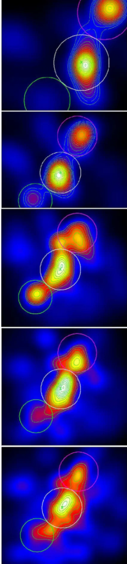
3.3. Defining regions in Ophiuchus through density maps GLFs have been observed to vary with the position within the cluster (e.g.Adami et al. 2007and references therein). In order to define the regions where it would be interesting to derive GLFs, we computed galaxy density maps based on an adaptive kernel technique with a generalized Epanechnikov kernel as suggested bySilverman (1986). Our method is based on an earlier version developed by Timothy Beers (ADAPT2) and further improved by
Biviano et al.(1996). The statistical significance is established by bootstrap resampling of the data. A density map is computed for each new realisation of the distribution. We choose a pixel size of 0.001◦(3.6 arcsec). For each pixel of the map, the final value is taken as the mean over all realisations. A mean bootstrapped map of the distribution is thus obtained. The number of bootstraps used here is 100.
The significance level of our detections was estimated from the mean value and dispersion of the background of each image. To estimate these quantities, we draw for each density map the histogram of the pixel intensities. We apply a 2.5σ clipping to eliminate the pixels of the image that have high values and cor-respond to objects in the image. We then redraw the histogram of the pixel intensities after clipping and fit this distribution with a Gaussian. The mean value of the Gaussian gives the mean background level, and the width of the Gaussian gives the dis-persion, that we call σ. We then compute the values of the contours corresponding to 3σ detections as the background plus 3σ. The contours shown in Fig. 7 start at 3σ and increase by 1σ.
The limitation here is that we only have photometry in one band, so we cannot select galaxies along the red sequence (i.e. with a high probability of belonging to the cluster). We therefore chose to compute maps for different magnitude limits (chosen arbitrarily), applied to the magnitudes before any extinction cor-rection: r0< 15.5 (25 galaxies), r0< 16 (58 galaxies), r0< 17 (141 galaxies), r0< 18 (271 galaxies), and r0< 19 (517 galaxies).
Obviously, the contamination by background galaxies becomes larger as the limiting cut becomes fainter.
The resulting density maps are shown in Fig.7. Since the galaxy catalogues from which the density maps are computed have slightly different sizes, the maps also have somewhat differ-ent sizes. However, the radii of the three circles remain constant from one figure to another.
We can see that depending on the magnitude cut, the aspects of the density maps change. The cluster (white circle) is clearly the brightest structure in all the maps. However, a structure is visible northwest of the cluster, and a second structure appears at fainter magnitudes southeast of the cluster.
We therefore defined three circular regions in which we derived the GLFs: the first one (hereafter C) is centred on the cluster centre and has a radius of 10.0 arcmin, or 351 kpc at the cluster redshift (white circle), the northwest circle (hereafter NW) is centred on RA = 257.9774◦, Dec = −23.0701◦ and has a radius of 9.7 arcmin, or 340 kpc (magenta circle), and the southeast circle (hereafter SE) is centred on RA = 258.3224◦,
Dec = −23.5961◦ and has a radius of 8.3 arcmin, or 291 kpc (green circle).
We note that the NW region more or less coincides with the zone whereWatanabe et al.(2001) found an excess of X-ray
Fig. 7.Galaxy density maps with various magnitude limits (chosen
arbi-trarily, for magnitudes without any extinction correction). From top to bottom: r < 15.5 (25 galaxies), r < 16 (58 galaxies), r < 17 (141 galax-ies), r < 18 (271 galaxgalax-ies), and r < 19 (517 galaxies). Contour levels start at 3σ above the background (see text) and are spaced by 1σ. The cross indicates the position of the cD galaxy.
Fig. 8. Galaxy luminosity functions in the Centre C (two top fig-ures), and in regions NW (two middle figures) and SE (two bottom figures) (see text). For each region, the top figure was obtained with a constant Galactic extinction and the bottom one with a different extinc-tion correcextinc-tion for each galaxy. Left: subtracextinc-tion of Yasuda background counts, and right: subtraction of Yasuda background counts multiplied by f = 0.7 (see Sect.3.1). The line colours are as in Fig.5.
emission in their ASCA image (see their Fig. 5), so it is probably a substructure in the cluster.
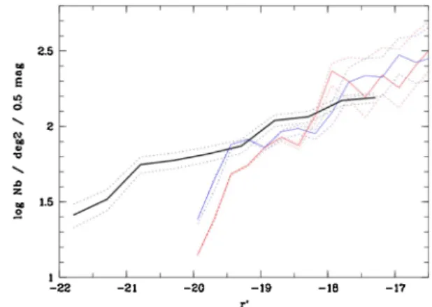
Fig. 9.Comparison of the GLFs of Ophiuchus (computed with variable
extinction and f = 1.0) and Coma in regions with the same physical sizes. The Ophiuchus GLF is in black, while the GLFs of the North and South zones of Coma are in red and blue, respectively. The dotted lines show the ±1σ errors on each curve.
3.4. The galaxy luminosity function in three regions
We extracted galaxy counts in the three circular regions, C, NW, and SE, and applied to each the two extinction corrections described above, and the two possible values for the background subtraction ( f = 1.0 and f0= 0.7).
The surfaces covered by the regions C, NW, and SE are 0.087468, 0.082725, and 0.060056 deg2, respectively. The GLFs are plotted in Fig.8and the fit parameters are given in Table1.
In region C, which corresponds to the cluster core, the impor-tance of the Gaussian component is strong, as it was for the overall cluster (see Sect.3.1) and in the “rectangle” region. The faint end slope is somewhat flatter in region C than in the overall cluster. Region C is therefore dominated by bright galaxies, as for region “rectangle”.
In view of the shapes and poor qualities of the GLFs in regions NW and SE, due to the low numbers of galaxies in these regions, no Gaussian function needs to be included for f = 1.0. In fact a simple power law would be sufficient to fit the GLFs, since in most cases M∗is not constrained. This implies that very bright galaxies are concentrated in the inner zones of the clus-ter, as expected, and that there are very few bright galaxies in the outer regions. The faint end slopes of the GLFs in regions NW and SE are close to those found for the overall image. We also note the importance of the Galactic extinction correction that somewhat modifies the parameters of the GLFs, in particu-lar in the SE zone, where the extinction has a particu-larger value (see Fig.2). For f0= 0.7, the GLFs in regions NW and SE look much
better, as expected, and the Gaussian component again appears necessary to account for the excess of bright galaxies.
4. Discussion and conclusions
Due to its low Galactic latitude, the Ophiuchus cluster is difficult to study at optical wavelengths. However, based on a photomet-ric catalogue of 2818 galaxies in a zone covering 1 deg2around
Ophiuchus, we have succeeded in obtaining the GLFs in the overall image, in a region (the “rectangle” region) of the same physical size as that considered for the Coma cluster byAdami et al.(2007), as well as in three circular regions defined from density maps: a central zone (C), and two regions northwest (NW) and southeast (SE) of the centre. In all the regions, the GLFs show an excess of very bright galaxies over a Schechter
A&A 613, A20 (2018)
function that is well fit by a Gaussian. The faint end slope is quite flat in the very central region C: between −0.58 and −0.83, while it is steeper in the outer zones. However, we must note that the GLFs of zones NW and SE are rather noisy, and that the choice of the correction for Galactic extinction and of the factor by which to multiply the background counts modifies the best fit parameters, so it is difficult to draw conclusions for these zones.
Since Ophiuchus and Coma are two massive nearby clus-ters, it is quite logical to compare their properties. The former is known to be quite relaxed (see e.g. Paper I) while extensive studies of the latter imply that it is far from relaxed and still undergoing one or several mergers. Therefore, the comparison of these two clusters can provide information on the effect the environment may have on their properties.
As explained above, we have extracted the Ophiuchus GLF in a region covering the same physical size (roughly 1.1 × 1.4 Mpc2) as the region in which the Coma GLF was calculated byAdami et al.(2007). The GLFs of Ophiuchus (com-puted for f = 1.0) and of the North and South halves of Coma computed in regions of identical physical size are shown in Fig.9. We can see from this figure that the GLFs are quite similar for galaxies fainter than Mr0 ∼ −19.5, but that Ophiuchus shows
a large excess, with respect to Coma, of galaxies brighter than Mr0 ∼ −19.5. The North region of Coma is known to contain a
large fraction of faint galaxies, while the South region of Coma, which is in contact with a large-scale filament arriving from the South-West, contains more bright galaxies. Ophiuchus contains many more bright galaxies than the South region of Coma, thus requiring mergers of quite massive galaxies.
One explanation could be that in the core of Ophiuchus many galaxy mergers take place. This agrees with the flatter faint end slope of the GLF in region C, relative to the two adjacent regions (NW and SE), and relative to the cluster at a larger scale (in particular the Overall region, see Table1).
Mamon (1992) showed that for a galaxy of mass m, the merging rate in a cluster varies as m2/σ3
v, where σvis the cluster velocity dispersion. The respective velocity dispersions of Ophi-uchus and Coma are approximately 950 km s−1 (Paper I) and 1200 km s−1 (Adami et al. 2009), so the ratio of the merging
rates in Ophiuchus and Coma for a galaxy of given mass m is expected to be ∼(1200/950)3= 2.0. At the absolute magnitude
Mr = −20, there are roughly three times as many galaxies in
Ophiuchus as in Coma (Fig.9). To obtain this factor of three, the ratio of the masses of bright galaxies in Ophiuchus and in Coma would therefore need to obey the relation (mOph/mComa)2 ∼ 3/2,
corresponding to bright galaxy masses in Ophiuchus mOphlarger
than the galaxy masses in Coma mComa by about 20–25%;
val-ues which are plausible. This very simple order of magnitude calculation shows that numerous galaxy mergers in the centre of Ophiuchus can indeed probably account for the very high number of galaxies brighter than ∼−19.5.
Another explanation to the high number of mergers could be that because Ophiuchus is embedded in a large-scale sys-tem involving the Great Attractor, this could favour galaxy– galaxy interactions and mergers. Such mergers could involve bright field galaxies of comparable masses and/or galaxies with small relative velocities, favouring efficient energy exchange between these galaxies, and forming even brighter merged objects.
We note however that, though being a very rich and mas-sive cluster, Ophiuchus does not appear to be embedded in a very dense network of galaxies, and its environment does not appear to be dense (Wakamatsu et al. in prep.). On the other hand, the large-scale environment of Coma, which is also a very rich cluster, at a comparable redshift, shows a much higher galaxy density. In the current paradigm where clusters are at the intersection of cosmic web nodes, it is somewhat difficult to understand how two massive clusters have built up to be of com-parable mass and richness within such different environments. The only explanation we see is that Ophiuchus has built up long ago, as confirmed by its relaxed state (see paper I), while Coma is still in the process of forming, as illustrated by the series of papers by Adami et al. (see e.g.Adami et al. 2007). It would be interesting to test this hypothesis by comparing the degree of relaxation and the large-scale galaxy distribution for a large sample of rich clusters.
Acknowledgements.We thank the referee for her/his very useful comments. We acknowledge enlightening discussions with Emmanuel Bertin. We are extremely grateful to Andrea Biviano for giving us, and adapting for us, his program to fit the galaxy luminosity functions, for pointing out theYasuda et al.(2001) paper, and for helpful discussions. We thank Florian Sarron for his help in extracting the individual extinctions for all the galaxies and Vincent Caillé for help mea-suring some of the galaxy magnitudes. F. D. acknowledges long-term support from CNES. J. M. O. M. M. M. was supported by the Brazilian agency CAPES (“Science without Borders” program 88888.789740/2014-00). This work is based on data obtained with MegaPrime/MegaCam (proposal 10AF02), a joint project of CFHT and CEA/DAPNIA, at the Canada-France-Hawaii Telescope (CFHT) which is operated by the National Research Council (NRC) of Canada, the Insti-tut National des Sciences de l’Univers of the Centre National de la Recherche Scientifique of France, and the University of Hawaii. This research has made use of the NASA/IPAC Extragalactic Database (NED) which is operated by the Jet Propulsion Laboratory, California Institute of Technology, under contract with the National Aeronautics and Space Administration.
References
Adami, C., Durret, F., Mazure, A., et al. 2007,A&A, 462, 411
Adami, C., Le Brun, V., Biviano, A., et al. 2009,A&A, 507, 1225
Bertin, E., & Arnouts, S. 1996,A&AS, 117, 393
Biviano A., Durret, F., Gerbal, D., et al. 1996,A&A, 311, 95
Cameron, L. M. 1990,A&A, 233, 16
Durret, F., Laganá, T. F., Adami, C., & Bertin, E. 2010,A&A, 517, A94
Durret, F., Laganá, T. F., & Haider, M. 2011,A&A, 529, A38
Durret, F., Perrot, C., Lima Neto, G. B., et al. 2013,A&A, 560, A78
Durret, F., Wakamatsu, K., Nagayama, T., Adami, C., & Biviano, A. 2015,A&A, 583, A124
Fukugita M., Shimasaku, K., & Ichikawa, T. 1995,PASP, 107, 945
Johnston, M. D., Bradt, H. V., Doxsey, R. E., et al. 1981,ApJ, 245, 799
Mamon, G. A. 1992,ApJ, 401, L3
Martinet, N., Durret, F., Guennou, L., et al. 2015,A&A, 575, A116
McCracken, H. J., Radovich, M., Bertin, E., et al. 2003,A&A, 410, 17
Press, W. H., & Schechter, P. 1974,ApJ, 187, 425
Schlafly, E. F., & Finkbeiner, D. P. 2011,ApJ, 737, 103
Schlegel, D. J., Finkbeiner, D. P., & Davis, M. 1998,ApJ, 500, 525
Silverman, B. W. 1986, Density Estimation for Statistics and Data Analysis
(London : Chapman & Hall)
Tully, R. B., & Fisher, J. R. 1987,Nearby Galaxy Atlas(Cambridge: University Press)
Wakamatsu, K., & Malkan, M. A. 1981,PASJ, 33, 57
Wakamatsu K., Malkan, M. A., Nishida, M. T., et al. 2005,Nearby Large-Scale Structures and the Zone of Avoidance, eds. K. P. Fairall, & P. A. Woudt, ASP Conf Ser, 329 189
Watanabe, M., Yamashita, K., Furuzawa, A., Kunieda, H., & Tawara, Y. 2001,
PASJ, 53, 605
Werner N., Zhuravleva, I., Canning, R. E. A., et al. 2016,MNRAS, 460, 2752
Yasuda, N., Fukugita, M., Narayanan, V. K., et al. 2001,AJ, 122, 1104
Appendix A: Typical errors on the magnitudes
Table A.1. Typical errors on the measured magnitudes depending on the magnitude range.
Magnitude range Error on magnitude r0< 20.0 0.05
20.0 < r0< 21.0 0.10 21.0 < r0< 22.0 0.20 22.0 < r0< 23.0 0.5
23.0 < r0 0.8
The typical errors on the measured magnitudes are given in TableA.1for various magnitude ranges.
Appendix B: The first ten lines of the photometric catalogue
The first ten lines of the photometric catalogue are shown in TableB.1.
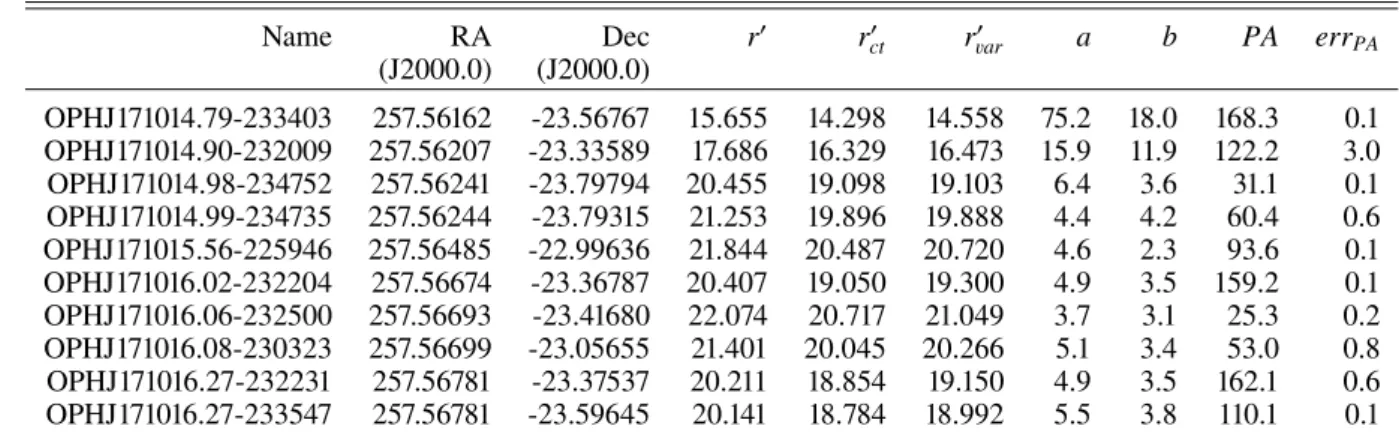
Table B.1. First ten lines of the photometric catalogue of Ophiuchus, which includes 2818 galaxies and is available in ViZieR at the CDS.
Name RA Dec r0 rct0 rvar0 a b PA errPA
(J2000.0) (J2000.0) OPHJ171014.79-233403 257.56162 -23.56767 15.655 14.298 14.558 75.2 18.0 168.3 0.1 OPHJ171014.90-232009 257.56207 -23.33589 17.686 16.329 16.473 15.9 11.9 122.2 3.0 OPHJ171014.98-234752 257.56241 -23.79794 20.455 19.098 19.103 6.4 3.6 31.1 0.1 OPHJ171014.99-234735 257.56244 -23.79315 21.253 19.896 19.888 4.4 4.2 60.4 0.6 OPHJ171015.56-225946 257.56485 -22.99636 21.844 20.487 20.720 4.6 2.3 93.6 0.1 OPHJ171016.02-232204 257.56674 -23.36787 20.407 19.050 19.300 4.9 3.5 159.2 0.1 OPHJ171016.06-232500 257.56693 -23.41680 22.074 20.717 21.049 3.7 3.1 25.3 0.2 OPHJ171016.08-230323 257.56699 -23.05655 21.401 20.045 20.266 5.1 3.4 53.0 0.8 OPHJ171016.27-232231 257.56781 -23.37537 20.211 18.854 19.150 4.9 3.5 162.1 0.6 OPHJ171016.27-233547 257.56781 -23.59645 20.141 18.784 18.992 5.5 3.8 110.1 0.1
Notes. The columns are: (1) name, (2) RA (2000.0), (3) Dec (J2000.0), (4) measured r0
band magnitude with no extinction correction, (5) and (6) magnitudes r0
ctcorrected for a constant value of 1.357 mag, and r 0
varcorrected for the individual extinction correction, (7) and (8) major axis a
and minor axis b in arcseconds (the error bars on these two quantities are typically 0.1 arcsec, so they are not given for every galaxy), (9) position angle PA of the major axis, (10) error on the position angle. We do not give individual errors on the observed magnitudes, but their typical values are given in TableA.1.