Analysis and visualization of equilibrium in masonry structures

Analysis and Visualization of Equilibrium in

Masonry Structures

by

Hijung Valentina Shin

Submitted to the Department of Electrical Engineering and Computer

Science

in partial fulfillment of the requirements for the degree of

Master of Science in Computer Science and Engineering

at the

MASSACHUSETTS INSTITUTE OF TECHNOLOGY

February 2014

@

Massachusetts Institute of Technology 2014.

ARCHIVES

iMASSACHUSETTS

WNS MUTE

OF TECHNOLOGY

APR 10 2014

BRAR1ES

All rights reserved.

A uthor...

..

Department of Electrical Engineering and Computer Science

y 27, 2014

Certified by ...

Professor of Electrical Engineering and

Fredo Durand

Computer Science

Tlgsis Skupugr

C ertified by ...

John A. OchKndorf

Professor of Architecture

Thesis Supervisor

A ccepted by ...

/Leslid Klo dziejski

Chairman, Department Committee on Graduate Students

Analysis and Visualization of Equilibrium in Masonry

Structures

by

Hijung Valentina Shin

Submitted to the Department of Electrical Engineering and Computer Science

on January 27, 2014, in partial fulfillment of the

requirements for the degree of

Master of Science in Computer Science and Engineering

Abstract

This thesis presents novel analysis and visualization methods to explore the

equilib-rium of masonry structures. Following a previous approach, we model the stability

problem as a quadratic program. When a structure is unstable the quadratic program

returns a measure of infeasibility. We extend this model to include tensile structures

such as cables. Then, we derive a closed-form gradient of stability with respect to

geometry modifications, and apply it to the design of structurally sound buildings.

In addition, we analyze various properties related to the equilibrium state of

struc-tures and visualize the result. We study the sensitivity of equilibrium with respect

to block weights, and from that we trace the flow of forces in the structure.

Finally, we compare the equilibrium approach to the finite element analysis (FEA)

method-the most widely used alternative. We point out the disadvantage of FEA

that comes from formulating the contact constraints and propose an improvement

based on an iterative constraint relaxation algorithm.

Masonry analysis; Statics; Equilibrium analysis; Structural optimization; Stability

visualization;

Finite element analysis; Contact constraints

Thesis Supervisor: Fredo Durand

Title: Professor of Electrical Engineering and Computer Science

Thesis Supervisor: John A. Ochsendorf

Acknowledgements

First of all, I would like to thank my advisor, Professor Fr6do

Du-rand and my co-advisor, Professor John Ochsendorf for their wisdom, patience, enthusiasm and support through my research at MIT. I am particularly grateful to them for allowing me to explore and develop my ideas, not only with their patient support, but also with their clear and to-the-point feedback. I will always value the many hours we spent discussing new ideas. It is a wonderful privilege to work with both professors. I dedicate this work to them.

I am indebted to Professor Thomas Funkhouser, who introduced me

to the field of computer graphics and inspired me to pursue research in graduate school. I am extremely grateful for his constant

encour-agement and friendship.

Numerous colleagues kindly helped me, and I would like to thank Emily Whiting and Etienne Vouga in particular, both of whom I turned to on many occasions. I am also grateful to David Levin, Sylvain Paris, Desai Chen for their timely advice and generous assistance at various stages of my research. I would like to thank Yichang Shih for his con-stant optimism and encouragement.

I am pleased to acknowledge the Samsung Scholarship Foundation for

their very generous financial support, which offered me the chance to come to this stimulating institute and meet many amazing people.

I would like to thank all of my friends who have taught me so much

about life, and especially my chavruta, Adriana Schulz. Most of all, I would like to thank my family, both near and far, for their unending support and encouragement.

Contents

Introduction Introduction

13

. . . . 13

Problem statement and contributions 14 Related works 15 Structural analysis . . . . 15

3D structure visualization . . . . 16

Equilibrium Analysis Static equilibrium analysis . . . . Analytic structural gradient . . . . Extension to tension elements . . . . Application to design of structures . . . . Future work . . . . 17 . . . . 17 . . . . 18 . . . . 18 . . . . 19 . . . . . . . . 21 Visualization of Equilibrium 23 Block weights . . . . 23 Force flow . . . .. . . . . 27 Future work . . . . 28 Comparison of Equilibrium and Elastic Analysis

Linear elastic formulation . . . .. . . .. -. Tension failure . . . .. . . . .. .. . . .. .. .. Contact constraints & interpretation of tension . . .. . . . Towards a compression-only solution . . .. . . . . . . . Comparison to the equilibrium analysis . . . .. . . .

Future work . . . . . . . .. . . . . -. Conclusions Bibliography 31 31 33 34 35 36 37 39 41

List of Figures

1 Parameterization of forces for tension elements . . . . 19

2 Convergence of infeasibility metric . . . . 20

3 Optimization of design using structural gradients . . . . 21

4 Sensitivity analysis with respect to block weights . . . . . 24

5 Maximum weight of blocks in an arch . . . . 25

6 Minimum weight of blocks in a vault . . . . . . 25

7 Thrust lines and block weights . . . . . . . . 25

8 Necessary weights for equilibrium . . . . 26

9 _{Important weights within structures . . . .} 27

lo Visualization of force flow through blocks . . . . 28

11 Contact constraints in FEA formulation . . . . . .. 32

12 _{Equilibrium vs. elastic analysis of thin arch . . . . 33}

13 Mechanism of three hinged arch . . . . 34

14 Tension forces and contact constraints in FEA . . . . 36 15 Comparison results from equilibrium & elastic analysis . 37

List of Tables

Introduction

Introduction

Much of the world's most important architectural heritage consists of masonry structures. It may seem superfluous to point out that these structures are valuable even by the mere fact that they are ancient and that they still exist. However, as Heyman points in his article, The

Stone Skeleton, this observation has force when placed in the structural

context [Heyman, 19661. The survival of Gothic cathedrals reflect the consummate expertise of the medieval master builders that brought out such extreme stability in their structures.

Strange though it may seem, despite the great advancement in build-ing technology made since those times, the structural actions of these historical buildings still remain in large part a mystery. So much so that explaining even as simple a structure as an arch becomes a debate within the theory of structures. While computational techniques and

visualization tools have considerably broadened the range of possible analyses, when it comes to practice we are still limited to a number of standard approaches such as finite element analysis to compute stresses inside structures. A deeper understanding of the stability of masonry structures would be valuable not only for the restoration and preservation of historical buildings but also for the design of new structures. The question remains: how do we explain the stability of a structure?

This thesis explores that question. The thesis consists of three main parts. The first part is a condensed summary of the equilibrium anal-ysis method as presented in Whiting's thesis [Whiting, 2012], and an extension of this method to structures with tension elements. This part served as the basis for a paper presented in SIGGRAPH Asia [Whiting et al., 2012] and provides a starting point for this research. The second part consists of experiments in visualizing the equilibrium of 3D struc-tures. We tried to ask different types of questions in order to illustrate the static equilibrium of a 3D structure from various angles. In the course of this exploration, we faced the problem of static indetermi-nacy of masonry structures. This led us the third part of the thesis,

14

which consists of the comparison between linear elastic finite element analysis(FEA) and equilibrium analysis.

Problem statement and contributions

This thesis investigates computational and visualization tools to ex-plore the equilibrium of masonry structures. In this context, we make the following contributions: 1) We extend a previous equilibrium anal-ysis to include structures with tensile elements and apply it to the design of stable structures. 2) We present novel visualizations which

bring new insights about structural equilibrium. 3) Finally, we demon-strate the differences between the two most widely used methods for masonry analysis: the equilibrium analysis and the elastic analysis.

Related works

Structural analysis

Computational analysis of structural soundness of mechanical parts or buildings has been widely applied. In the context of computer graph-ics, stability analysis has been useful especially for animation and re-cently also for 3D modeling and printing. For example, [Shi et al., 2007] uses static equilibrium to determine realistic character poses. [Umetani et al., 2012] performs stability analysis in an interactive tool to design physically durable plank-based furniture. [Zhou et al., 2013] presents a method to identify structural problems for a broad range of objects designed for 3D printing. This thesis focuses on masonry structures and their equilibrium.

Approaches to masonry analysis can be broadly grouped into two cate-gories. Strength methods represented by finite element analysis (FEA) assess structures by computing its stress and taking into consideration the limits of material strength. FEA applied to masonry structures has been studied extensively. The reader is referred to [Tzamtzis and Asteris, 2003] for a comprehensive summary. A different approach proposed by Jacques Heyman [Heyman, 1966] is commonly referred to as limit state analysis. Based on three main assumptions 1) that masonry has no tensile strength, 2) that masonry can resist infinite compression, and 3) that no sliding will occur within the masonry, these methods assess stability only from the geometry of the structure. These methods assume that geometrical stability rather than material strength compared to stresses is key to structural soundness, and focus on attaining force equilibrium. For an extensive historical overview of equilibrium methods the reader is referred to [Huerta, 2008]. Here, we focus on several most relevant works.

Traditionally, equilibrium methods were applied to masonry using graphical techniques called graphic statics. Recently, [Block et al., 2006] created interactive graphic statics tools which suggested the possibility of using computerized graphical methods for the analysis of masonry structures. [Block and Ochsendorf, 2007] extended graphic statics to 3D masonry shells by introducing the Thrust Network Analysis (TNA)

16

method. Using projective geometry and dual force diagrams they find a compression-only structure from an input mesh and boundary con-straints. In the computer graphics community, in particular [Vouga et al., 2012] and [Panozzo et al., 2013] applied TNA to design and

op-timize unreinforced masonry structures.

This work is most closely related to and builds upon an alternative equilibrium method introduced by R.K. Livesley [Livesley, 1978], and further developed by Emily Whiting in her thesis [Whiting, 2012]. While TNA is specific to shell structures with topologies that can be projected onto a 2D plane, Whiting's method is applicable to arbitrary topologies. This thesis 1) extends the method to include tension-only elements, 2) applies it to develop visualizations of structural equilib-rium, and 3) compares it to the finite element analysis method.

3D structure visualization

Architects and engineers rely heavily on visual tools to illustrate 3D objects or environments in order to explain their parts, functions, spaces and structures. A good visualization is key to both understanding an existing structure and designing new structures.

In computer graphics and visualization, researchers have developed various techniques to explore different objects, each focusing on dif-ferent aspects. Some of them are concerned with illustrating the geom-etry of complex objects. For example, [Niederauer et al., 2003] present a system for interactively producing exploded views of 3D architec-tural environments such as multi-story buildings, and [Karpenko et al., 2010] visualize complicated mathematical surfaces using techniques inspired by hand-designed topological illustrations. Other works at-tempt to demonstrate the function of an object. For instance, [Mitra et al., 2010] introduce an automated approach for generating visual-izations that depict the operation of complex mechanical assemblies starting from their 3D models. [Shao et al., 20131 develop a system to facilitate exploration of product functions from their concept sketches. Still other works focus on depicting properties inside ₃D objects. [Dick et al., 2009] visualize stresses inside bones under load to facilitate or-thopedic surgery, and [Laramee et al., 2005] visualize fluid flow inside cooling jackets in order to investigate and evaluate the design of an automotive engine.

Most visualizations are application specific and require some knowl-edge about the object or environment. To a certain extent, this is in-evitable since both what and how to visualize are determined by the application. The second part of this thesis focuses on visualizing dif-ferent aspects of equilibrium in masonry structures with the goal of gaining a better understanding about how structures stand.

Equilibrium Analysis

Static equilibrium analysis

In her thesis, Whiting develops a structural analysis method by ex-tending an approach introduced by [?]. This method formulates the static equilibrium problem-i.e. whether a structure is in equilibrium or not-as an optimization problem under linear constraints. Here, I provide a condensed summary of the method and deal with its exten-sion to tenexten-sion elements in more detail. For a thorough explanation of the method, I refer the readers to [Whiting, 2012].

Whiting models structures as assemblage of rigid blocks, and dis-cretizes the force distributions at the interfaces between these blocks. We place a 3D force fi at each vertex of the interface. Each force fi is decomposed into three components with respect to the local coordi-nate system of the interface: a normal component,

fn

and two in-plane friction components, orthogonal to each other,

fi"

and

f].

The normal and friction forces on a shared interface between two blocks have op-posite orientation for each block.

The stability analysis, also commonly referred to as limit analysis, lies on three basic assumptions of masonry behavior introduced by [Hey-man, 19661. They are: (i) Masonry has no tensile strength; (2) stresses are so low compared to material strength, that masonry has effectively unlimited compressive strength; and (3) sliding failure does not occur. Finally, the safe theorem of the plasticity theory states that if one pos-sible, lower bound, solution can be found that satisfies equilibrium, the structure will be safe, i.e. it will stand. Under these assumptions the static equilibrium can be expressed as a linear system as follows.

minimize g(f) =-

fTHf

f

2

subject to Aeq -f = -w (1)

f > 0

The first equality constraint enforces that the net force and net torque for each block is equal to zero. w is a vector containing the weights of each block, f is the vector of interface forces and Aeq is the sparse matrix of coefficients for the equilibrium equations. The second inequality constraints apply to normal forces and enforce the forces to be compressive. Finally, the equality constraint Afr - f = 0

approx-imates the friction cone constraints.

If

1, 1f I <

af

, Vi E interface vertices.

If a solution

f

exists that satisfies all the constraints, the structure is in equilibrium. Otherwise, the structure is unstable. Furthermore, by softening the compression-only constraint and allowing tension forces, it is possible to solve for the forces of infeasible structures. In this case, H is a diagonal weighting matrix of forces, which places a large penalty on the tension forces and low penalty on the remaining forces. [Whiting, 2012] uses the function value

ifTHf

as a measure of infeasi-bility of a structure.

Analytic structural gradient

After formulating the static equilibrium problem as a linear optimiza-tion and defining a measure of infeasibility of a structure, [Whiting, 2012] derives its closed-form derivative with respect to the displace-ments of the vertices describing the structure geometry. The gradient expresses how the infeasibility of a structure changes with respect to changes in the structure geometry.

Extension to tension elements

Whiting's approach can handle other types of constraints such as those corresponding to tension-only elements. I extended the method to in-clude cables in structures. Whereas the same principles of static anal-ysis and gradient computation apply, cables are different from rigid blocks in several ways:

1. Cables can resist tension, but fail under compression. I model cables with infinite tensile capacity, and penalize compression forces. 2. There are no friction constraints. The cables are modeled as

in-finitely thin elements that are firmly attached to each other or to a block.

3. Cables can apply forces only along their axis. This means that a structure can be infeasible not only due to the sign of the required forces (i.e. compression inside cables or tension in between blocks),

19

but because of their limited degrees of freedom. For example, Fig-ure 1 shows a case where there is no configuration of forces along the cable axis that achieves static equilibrium. In order to compute a measure of infeasibility for such structures, I define virtual torques around the centroid of each element and include them in the penalty function.

The geometry of each cable is defined by its two end points {Po, P1} which may be attached to an adjacent cable or to a point on a block surface. The direction of the tension force,

ft,

is along its axis. Similar to blocks,

f'

is split into positive and negative components,

f+1,

and

ft.

Compression,

f+f

is penalized for cables. It is possible to place an upper bound on

ft

with inequality constraints, which reflect the scale of the cable since strength is relative to cross-sectional area.

Cable elements are assigned a weight, w = pLg, where

L

is the length of the cable and p is the mass per unit length. For gradient com-putation, we parameterize cables using the x, y, z coordinates of their end points. In order to compute the structural gradient, we need the derivative of the weight vector, and the derivative of the cable tension direction (it) with respect to the position of its end points (w). The derivative of the weight vector aw/w for cable is given by:

aw

U

L

1(po

- pi) - O

aw

2 |po-pil

where coordinates po, p1 are two ends of the cable. The derivative of the cable tension direction is

a

PO - Pi

Ca

w

_{a w}

_||,

_p

_'

_{- p 1}

_||-

P ll

|HPO

-

P1||H(

-

(PO-

P1) -

(

g

)

flpo

- pi2

cable

A, t

_t

ty Wbock

Figure 1: The tension force f t applied

by the cable balances the block weight,

but creates unbalanced torque. Virtual torques are added in directions ix, ty,

and iz around the centroid of the block to solve for static equilibrium.

(2)

(3)

(4)

(5)

For details on how to derive the analytic structural gradient please

see [Whiting, 2012].

Application to design of structures

In the design process of a structure, it is customary to perform struc-tural analysis only after the aesthetic design has been determined. An architect designs the shape and then passes it to structural engineers who try to make the structure stand using appropriate material and reinforcement. In contrast to this type of approach, [Whiting, 2012]

20

suggests using the structural gradient to directly suggest ways to im-prove the geometry in order to enhance structural soundness in the design process.

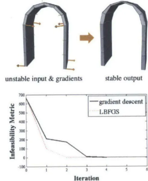
Given an infeasible structure, the structural gradient informs how to modify the geometry (i.e. move the block or cable vertices) in ways to improve feasibility. The following figures show examples of infeasi-ble input structures and their modifications to a stainfeasi-ble configuration. In modifying the structure, only geometric changes are considered. Topological changes such as attaching or detaching a cable are not considered. Most results are achieved after a number of iterations. Again, Whiting's thesis provides details of the implementation con-cerning geometry modification.

Figure 2: Progress of the infeasibility metric as the unstable arch is modified into a stable structure. At each iteration the value of the infeasibility decreases and converges toward 0 after a small number of gradient steps. The perfor-mance is improved further by L-BFGS.

unstable input & gradients stable output

700 0 -gradient descent 5s00 LBFGS

~400--300 200 100 0 1 2 3 4 5

Iteration

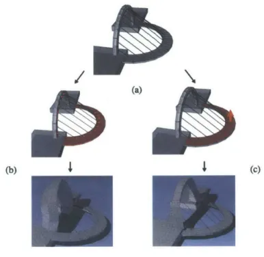
In addition to computing the first-order gradient, I implemented the limited-memory Broyden-Fletcher-Goldfarb-Shanno method (L-BFGS) for non-linear optimization [Fletcher, 1987]. L-BFGS searches for the minimum by approximating the Hessian matrix, using the first-order gradient. Experience suggests that L-BFGS converges to a stable so-lution with fewer iterations than using only the first-order gradient directly (Figure 2), particularly for models with higher complexity. Figure 3 demonstrates an example of using the structural gradient to optimize a cable-stayed bridge design. The input bridge is unstable because the horizontal walkway is too heavy for the vertical arch to hold up. In the first case, we fix the horizontal walkway and the po-sition of the cables, and only modify the vertical arch. After several

21

iterations we arrive at a stable solution, where the arch has thickened and leaned backwards to balance the torque. In the second case, we allow the horizontal walkway to deform, as well as changing the posi-tion of the cables. As the funcposi-tion of the bridge requires, we constrain the top surface of the walkway to remain horizontal. Now, the bridge is optimized to a different stable structure, where the vertical arch has significantly thickened, the base arch has become thinner in the middle and thicker at the supports.

Figure 3: An example of optimizing a structure to improve stability (a) A cable-supported bridge structure origi-nally infeasible. (b) Constraint and cor-responding feasible output. The hori-zontal arched walkway and cables are fixed and only the vertical arch is mod-ified. (c) An alternative feasible output, where only the normal of the arch

walk-(a) way is fixed to remain horizontal.

(b) (c)

Future work

The feasibility or infeasibility of the linear program in equation (1) gives us a binary answer to whether a structure is stable or not. When the structure is unstable, the sum of tensile forces gives a continuous metric of infeasibility. It would be useful to develop similar metrics to indicate the degree of stability for stable structures.

In computing the structural gradient, we considered only geometric changes to improve stability. However, increasing stability in this way does not guarantee a feasible solution and topological changes may be necessary. It would be interesting to consider, for example, optimizing

for the number of cables or blocks.

Along with structural gradients, user constraints and user-defined ob-jectives presented in [Whiting et al., 2012] provide a useful tool to

22

guide structurally stable designs. However, there is still much room

for improvement in the area of interactive design and optimization. For example, it would be valuable to combine editing and visualiza-tion algorithms presented in 3D modeling tools such as [Igarashi and

Hughes, 2001] and [Gal et al., 2009] with analysis and optimization

Visualization of Equilibrium

According to Heyman's safe theorem, the existence of an equilibrium solution for a structure indicates that the structure can indeed stand. Yet, this is just one answer that leads to many more questions. For example, how stable is the stable structure? Can we quantify this sta-bility? How is the equilibrium affected by perturbations? What does the equilibrium state consist of? In other words, we are interested in not only whether the structure is standing or not, but how it is standing. The challenge here lies as much in formalizing what we mean by how as in obtaining and visualizing the result. This section takes a first step in exploring this topic.

Block weights

In the previous chapter, the equilibrium of a structure was expressed as a series of equality constraints enforcing the equilibrium of individ-ual blocks. In the absence of external forces, the right hand side of

Aeq - f = -w becomes a vector containing the weight of each block.

One approach to studying the equilibrium is to do a sensitivity analy-sis with respect to these block weights. We ask how the force solution,

f, changes with respect to variations in w.

Computing the analytic gradient

Vfwi

is similar to computing the ana-lytic structural gradient. We use the closed form expression of the force

solution derived in [Whiting et al., 20121. The closed form expression

is derived for a given geometry 0, by fixing the active constraints and transforming them into equalities at the local solution:

fn

= H-1CT(CH- CT)-lb (6)

C is a concatenation of the static equilibrium constraints and the active inequality constraints, and b is the concatenation off -w and o for the active inequality constraints. Then the expression for the derivative of fn with respect to the i-th block's weight wi is:

n =H-1 CT (CH-CT)-lbi ₍₇₎

24

where bi is a vector containing all zeroes except 1 for the i-th block's weight.

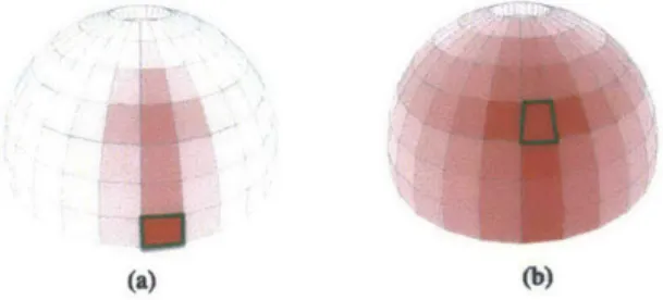
Figure 4: Force change with respect to increase in block weights for a dome structure. (a) Making the bottom block heavier does not significantly affect the rest of the structure. (b) The block in the middle, on the other hand, affects the forces on the blocks below and around it.

(a) (b)

Figure 4 shows examples from the sensitivity analysis on different blocks of a dome. The force gradient is computed with respect to the weight of a selected block. The results show blocks color coded by the total change of forces acting on their interface. The colored area can be interpreted as the sphere of influence of the selected block. As expected, in the case of the bottom block, changing its weight does not signif-icantly affect the forces in the rest of the structure. The small force change in the blocks above it indicated by the slight red is a side effect of using a L2-norm for the objective function. That is, the objective in (1) tries to minimize the sum squared forces by distributing the forces equally as much as possible. Therefore, when we increase the weight of the bottom block, the weights of the blocks above it are distributed more to the sides in order to balance the forces at the ground inter-faces. On the other hand, when we increase the weight of the block in the middle of the dome the added weight is transmitted to the blocks below it and around it, increasing both the longitudinal arching forces and the latitudinal hoop forces.

A related question is: how much can we increase or decrease the weight of a block while preserving equilibrium? We approach this problem by a brute-force method. For each block, we decrease or in-crease its weight and solve the optimization in (1) until the problem becomes infeasible. Figure 5 shows the maximum load of each block in an arch. Not surprisingly, the blocks at the supports of the arch can carry large weight. More interesting is the crown of the arch. It has slightly larger load capacity than the blocks to its side. Figure 6(a) shows the minimum load of each block in a vault supported by flying buttresses. Only the outer buttresses need weight in order to resist the outward thrust of the vault. However, as Figure 6(b) illustrates our analysis is too local and the results depend on the discretization of the structure. If the buttress is subdivided into smaller blocks, only

25

the top blocks need weight. If we subdivide these blocks even further, no individual blocks would need weight. As long as the other blocks have weight, the buttress as a whole can stand. A different type of analysis would be necessary to probe the nature of the structure that is independent of discretization.

Figure 5: Maximum weight of blocks of an arch. The supports near the bot-tom have large load capacity. The crown block also has slightly greater load ca-pacity than the blocks to its side.

1

Figure 6: Minimum weight of blocks in a vault supported by flying buttresses. (a) Weight is necessary only at the outer buttresses. (b) However, our analysis is sensitive to discretization. If we

sub-divide the outer buttress into smaller blocks, only the top block needs weight.

-j

\..

~,

(b)

The investigation about the minimum necessary weight of blocks leads to the following insight. There are at least two different roles that a block contributes to equilibrium. A block can provide a path for the transmission of forces through a structure, and/or it can deflect the force path by its weight. Figure 7 illustrates this idea using thrust lines. A thrust line represents the locus of internal reaction points found by determining the location of the interface force reactions required to maintain equilibrium [Ochsendorf, 2002]. Comparison of the two buttresses shows that the added weight on the top of the right buttress pushes the thrust line away from the outer edge of the wall, adding stability to the structure.

There are many ways to approach this question of distinguishing the different roles of each block in the equilibrium state. One way is to fix the block weight to be 0 and check if a feasible equilibrium solu-tion exists. If a solusolu-tion exists, the block is acting primarily as a path to transmit forces, and its weight has an insignificant effect. Another approach asks a slightly different question. For a single block with a fixed non-zero weight, we can ask what are the minimum necessary

Figure 7: Flying buttresses with the lines of thrust. Blocks transmit forces through the structure. (Right) The extra block

weight deflects the thrust line closer to the center of blocks.

I

_(a)

41

41

26

weights of the rest of the blocks that achieve equilibrium. The equilib-rium formulation becomes:

minimize h(x) = xTpIX

2

subject to Aeq -x = -W ₍₈₎

Afr

f

=

0

f

> 0,

wJ

> 0

where the variable x is a concatenation of the interface forces and the unknown block weights wj's, and * is a vector of all zeros except for the fixed block weight. Extra inequality constraints are added to en-sure that block weights must be nonnegative.

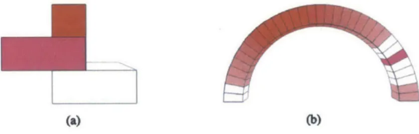
Figure 8 illustrates two examples. In the case of the stacked

Figure 8: Minimum necessary weights for equilibrium. In each case, only the highlighted block is assigned fixed weight. Red blocks need weight whereas white blocks only act as path to trans-mit forces. Red intensity indicates mag-nitude of necessary weight.

(a) (b)

blocks, the middle block has fixed weight. The top block must have positive weight in order to exert a downward force that balances the torque in the middle block. On the other hand, the bottom block need only transmit the forces downward to the ground. The case of the arch is more complex. In order to balance the torque of the high-lighted block, blocks on the opposite side need weight. This in turn creates thrust that is balanced by placing weights on the bottom right side. Similarly, in most structures there is a chain of dependency be-tween blocks, where in order to support one block another block needs weight, and in order to support that weight, yet another block needs

weight and so on.

Finally, by adding the minimum necessary weights computed with re-spect to each block in the structure, we could visualize which parts of the structure have weights that are significant for the equilibrium. Figure 9 presents the results for an arch and a dome. Weights are most important at the haunches of an arch. In real arches, this is some-times handled by placing concrete or rubble fillings on the haunch [Jagadeesh and Jayaram, 2000]. As expected, block weights do not have a significant role at the bottom and top of a dome.

27

Figure 9: Sum of the minimum neces-sary weights solved with respected ev-ery other block (normalized by block volume). Redder color indicates blocks that need weight in order to support other blocks.

Force flow

Underlying the previous considerations-about a block's weight de-flecting the thrust line or the weight of a single block being transmit-ted through other blocks-is the idea of the flow of forces within the structure. Force flow or load paths is a concept frequently used in the structural analysis of masonry. For example, [O'Dwyer, 1999] tries to identify the principal load path in order to compute a force network that represents the surface of thrust in a masonry vault. Similarly, in his thesis about Thrust Network Analysis, Block discusses the im-portance of choosing a network topology that can represent the force flows [Block, 2009].

We approach the problem of identifying force flows by considering the change in the force solution f in response to external forces. This idea was employed in section to access the sensitivity of the structure to block weights. This was useful, for example, to visualize the sphere of

influence of a particular block within a structure. Here, the goal is more

demanding. We would like to trace the weight of a single block (i.e. the force that the block exerts on the rest of the structure) through con-secutive adjacent blocks and eventually to the ground. This becomes a more local and sequential process. At each step, we are only con-sidering the flow of forces to adjacent blocks (or interfaces since that is where we represent the discrete forces in our model). If we have a method to trace forces from one interface of a block to the other, we can apply it recursively until the forces reach the interface at the ground.

We visualize the load path of a single block(B) as follows:

1. Start traces pointing downward from the center of mass of B. The number of traces is proportional to the weight of B. Each trace rep-resents a force with a location (center of mass) and direction (down-ward).

2. Compute the change in force solution df at B's interface with respect to the force represented by each trace.

3. Define a probability distribution on the interfaces of B according to df. Larger change in force means higher probability. The probability

28

is interpolated on the surface of the interface and normalized to add up to 1.

4. Trace each path to a point on an interface according to the probabil-ity distribution.

5. Each trace again represents a force with a location and direction defined at an interface. Repeat steps 2-4 for each trace recursively until it reaches the ground.

Figure lo presents two examples. The load traces illustrate that the weight of the middle block in the H structure is supported equally by the two columns, whereas the weight of the top block in the right structure is supported mostly by the left column. In the same manner, we could trace the weight of every block in a structure and superim-pose the traces. The density of the traces would show principal load paths where forces tend to concentrate inside the structure.

Figure 10: The weight of the selected

block (highlighted) is transmitted through

adjacent blocks into the ground. (a) Weight trace starting from the center of mass, and (b) starting from random sam-ples inside the block.

(a) (b)

Future work

The approaches suggested in this chapter are a first step towards bet-ter analysis and visualization of equilibrium in structures. There are many interesting and challenging aspects that are waiting to be devel-oped, some of which we hope to investigate in a continuation of this research.

Visualizing properties on 3D structures is in itself a challenging sub-ject. As we consider structures with increasing complexity and num-ber of blocks (e.g. a cathedral), the problems of occlusion, navigation and interactivity become more important. The choice of both what and how to visualize would affect the effectiveness of the result. For example, exploring volumetric or texture-based representation of force flows inside a structure, or a hierarchical representation depending on the required level of detail leaves much room for future investigation.

29

Developing computable metrics or definitions for the various quali-ties to visualize is also an important area. For instance, stability, force paths or interdependence between blocks are useful concepts, yet too vaguely used. The primary goal of visualization is to aid understand-ing about the state of the structure. Therefore, one startunderstand-ing point may be to consider applications and what information is useful for poten-tial users. For instance, a commonly used measure of stability is the tilt test, which measures the maximum angle of tilt before collapse ([Ochsendorf, 2002] and [Zessin, 2012]. Depending on the application,

other measures of stability would also be useful.

The equilibrium method presented in [Whiting, 2012] provides a use-ful way to do limit state analysis for masonry structures. However, it gives little clue about the actual force state. First, the objective function that is used to find the optimal force solution is not based on physical principles. It attempts to minimize total forces while penalizing ten-sion, but this is not an accurate description of how a structure finds equilibrium. It is not a question of finding a magical objective function either. Rigid body physics by itself does not specify enough infor-mation about the structure to determine one actual state for a given structure. In most cases, masonry structure is hyper-static or statically indeterminate, meaning an infinite number of equilibrium solutions exist. So, the question arises about how to deal with this inherent in-determinacy. Finite element analysis is one way, and this is where we turn to next.

Comparison of Equilibrium and Elastic Analysis

Finite element analysis (FEA) represents the most widely used method for structural analysis in many fields of engineering, including ma-sonry. However, recently, several studies pointed to the shortcomings of FEA and suggested that the problem is not only in the level of ac-curacy it attains but that the method is inherently inappropriate for

masonry structural analysis ([Whiting, 2012], [Block, 2005]). Instead

they propose equilibrium analysis such as the one presented in the previous chapters. Still, other than few example cases where FEA pre-dictions fail, to our knowledge, no attempt has been made at a clear and thorough explanation about why equilibrium analysis is more ap-propriate than FEA. This chapter examines the problem of FEA closely in order to clarify why it is not suitable for masonry. Based on our observation, we also propose an improved algorithm for FEA.

FEA divides a structure into many small elements and prescribes ma-terial properties to them in terms of stiffness matrices. It specifies boundary conditions on the displacements of the elements. Finally, based on variational principles, it computes the displacement of the elements, which are used to derive stresses and strains in the struc-ture. Masonry structures have several characteristics that make FEA challenging. For instance, [Whiting, 2012] calls attention to the fact that FEA is designed to model a continuum rather than a discontinu-ous set of blocks, that it does not consider the indeterminate property of masonry structures, and that stresses in masonry are low compared to material stiffness so elastic deformations are almost negligible. In what follows, we identify characteristic cases where FEA outputs

incorrect results and present a clear interpretation for the cause of its

failure. These cases also shed light on a possible step towards unified comparison of the FEA with the equilibrium analysis which we plan to follow up in future research.

Linear elastic formulation

First, in order to compare with the equilibrium method presented in previous chapters we formulate and implement a simple finite element

32

analysis as follows:

i. Each block constitutes a hexahedral element with eight nodes, one at each corner of the block. The stiffness matrix Ki is computed for each element. We use Ki =

f_

BTEBdV, assuming that the stress-strain matrix E is constant over the element. B is the strain-displacement matrix. The integral over the volume V is replaced by a numerical integration at the Gauss quadrature points. [Felippa and Clough, 1970]

2. The global stiffness matrix K is computed for the entire structure by assembling the Ki element matrices.

3. The principle of minimum total potential energy states that the structure will deform to a position that minimizes the total potential energy. From this principle, the FEA is formulated as an optimiza-tion problem:

minimize E (u) =

TKu

+ eu

U

2

₍₉₎

subject to An - u = 0

We are solving for the nodal displacements u. We use a linear elastic model. 1uTKu is the elastic potential energy, and eT u is the gravi-tational potential energy due to the weight of the blocks distributed to the nodes. Finally, the linear equality constraint An - u = 0 states the boundary conditions, described next.

4. The boundary conditions limit the space of allowable nodal dis-placements. In the physical world, blocks that are in contact cannot interpenetrate. The constraints ensure that adjacent nodes at an in-terface do not pass through each other. We express this by requiring their displacements to be the same. That is, for every pair of nodes pi and p1 that are adjacent at an interface, ui = up. (See Figure 11.)

5. Once we find the optimal solution u*, the elastic force is computed as fK = -Ku*. Similarly, the contact forces between elements is computed from the contact constraints and their Lagrangian multi-pliers so that fc =A

A-There are many ways to refine the method, for example by using smaller elements or a nonlinear stress-strain relationship. Our aim in formulating the FEA was to capture the essential characteristic of elas-tic analysis-elaselas-tic deformation of the material according to its prop-erty and the principle of minimum potential energy-in the simplest possible model.

Figure 11: Each pair of adjacent nodes

pi and pj at the interface is constrained to remain in contact and not penetrate through the other block. This is done by enforcing their displacements to be the same (ui = uj).

33

Equilibrium Elastic (FEA)

Assumptions rigid elements elastic elements safe theorem min total potential energy

Constraints YZ(force per block) = 0 ui = uj for nodes i,

j

E(torque

per block) = 0 in contact ff >

0

Friction Coulomb friction cone

oo

for contact nodes

0 if contact is released

Output forces displacements

Tension failure

Table i presents a summary of the two methods. Unlike the equilib-rium formulation, the elastic formulation does not give a direct answer as to whether the structure is stable or not. However, each contact con-straint (A', the i-th row of An) comes from an interface

j

between two blocks, and it gives rise to contact forces (f = Ai - (A') T) at the nodes. By comparing these contact forces with the interface normal (f -ni), we can check whether the force is compressive or tensile.

In pointing out the shortcomings of FEA, [Block, 2005] refers to the case of two arches, one thicker and the other thinner. Equilibrium analysis shows that the thicker arch has a compression-only equilib-rium solution, whereas the thinner arch is too thin to contain a thrust line and therefore would not stand under its own weight without ten-sile forces. However, FEA cannot reveal this major difference and out-puts very similar results for the two arches. In fact, Whiting points out that linear elastic FEA predicts tension for both arches despite the thicker arch having a compression-only equilibrium solution.

Table i: Comparison of equilibrium and elastic analysis

Figure 12: An example often pointed out as a failure case of FEA. (a) Elastic analy-sis predicts tension forces (highlighted) at

the crown where (b) equilibrium analy-sis finds a compression-only solution.

(a) Tension in elastic solution (FEA) (b) Compression-only equilibrium solution

We verify this result for an arch with thickness to radius ratio (t/R) of 0.12. This is sufficiently thicker than the theoretical minimum

re-quired for a stable arch, which is t/R = 0.1075 [Ochsendorf, .2006].

Figure 12 presents the result. Although the equilibrium analysis finds a compression-only solution, where the thrust line is completely

con-34

tained within the arch blocks (12b), FEA outputs a solution with ten-sion forces at the crown of the arch (12a).

Contact constraints & interpretation of tension

Now, let us take a closer look at the tension forces in FEA. We ob-serve that tensile forces in FEA should not be interpreted simply as a failure to find a compression-only solution. Rather, tensile forces in FEA indicate that the boundary condition does not correspond to the physical reality of the structure we are trying to model. We will see that, in fact, we must change the boundary condition to correspond to the structural reality, and then search for a compressive equilibrium solution.

As explained earlier, the constraint confines the space of allowable nodal displacements. Specifically, when adjacent blocks in compres-sion try to interpenetrate each other, the boundary condition prevents this from happening. This applies for nodes that are in compression, but the same is not true for nodes in tension.

Physically, blocks cannot interpenetrate, but they can separate from each other. This is an important difference between masonry struc-tures and other continuum strucstruc-tures modeled in traditional FEA. The element boundaries in continuum structures are artificial boundaries that have both compressive and tensile capacity. On the other hand, block interfaces are physical boundaries that have zero tensile capac-ity. It is perfectly possible for blocks to separate from each other. In fact, the artificial tensile forces appear precisely because blocks try to move away from each other, but false constraints do not represent this reality and incorrectly prevent nodes from separating.

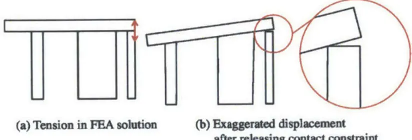
The arch in Figure 13 illustrates this case. At the top part of the crown interface (t), the blocks are pushing toward each other, so the non-penetration constraint applies. On the other hand, since the abutments of the arch give way with time, at the bottom part of the same interface (b), the blocks try to separate away. If the boundary condition does not express this reality, tensile forces appear. This is the case, even though the three-hinged arch is a perfectly stable configuration that is not at the point of collapse.

Previous works have alluded to this as a failure of FEA to find a compression-only equilibrium solution. However, this is because the boundary condition represents an incorrect physical model. We need to modify the boundary constraint to include hinging behavior in its feasible region. This is what we discuss next.

t

b

Figure 13: The arch is supported by an abutment, which will give way slightly. The lower figure, greatly exaggerated shows how the arch accommodates it self by developing three hinges. The arch is stable.

35

Towards a compression-only solution

The difficulty in forming the correct boundary condition comes from determining which nodes are in contact and therefore where the con-straints apply. If the nodes are trying to move toward each other, constraints must ensure that they remain in contact and not interpen-etrate. Otherwise, if they are trying to move apart from each other, the constraint must be released. However, it is impossible to know a priori which nodes should be constrained. To resolve this problem, we propose an iterative constraint relaxation algorithm inspired by simi-lar approaches developed for physical simulations.

Contact resolution is recognized as a fundamental challenge in multi-body dynamics. The problem comes from the coupling between fric-tion impulses and contact impulses. In order to compute the fricfric-tion impulses, contact points must be resolved. However, in order to deter-mine the contact points accurately friction impulses must be known. A recent approach proposed by [Kaufman et al., 2008] solves this prob-lem using a predictor-corrector method. First the predictor computes the contact points, and then the corrector uses this result to solve for friction. The two steps are interlaced until the system converges. Their algorithm is able to produce robust and accurate simulations of rigid and deformable bodies.

Following the same principle, we propose the following approach, in which we iteratively relax the contact constraints for nodes that de-velop tension forces.

1. First, FEA is solved with all the contact constraints present, requir-ing adjacent blocks to remain together.

2. The contact force f* is computed from the displacement solution u*,

its corresponding active constraints and their Lagrange multipliers (f* = AT -A).

3. If a contact force on a node is tensile, we release the constraint on that node by deleting the corresponding rows from An.

4. We solve for the modified FEA with fewer contact constraints.

5. Steps 2 to 4 are repeated until a compression-only solution is found, or until a maximum number of iterations is reached.

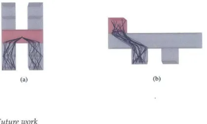
In several cases, we were able to find a compression-only FEA solu-tion where the initial solusolu-tion had predicted tension. For example, the arch in Figure 12 converged to a compression-only solution after two iterations. Figure 14 shows an example of a horizontal block supported by three columns. This is a stable configuration, where the weight of

36

the horizontal bar is distributed to the three columns. In the elastic so-lution, however, the leftmost column is thin and it shrinks more than the thicker middle column. This causes the horizontal bar to lean left-ward and the initial solution predicts a tensile force at the interface of the rightmost column. After releasing the contact constraint at this interface, FEA finds a compression-only solution. If we scale up the displacements of this solution, we observe a hinge where the initial solution predicted tensile forces.

(a) Tension in FEA solution (b) Exaggerated displacement after releasing contact constraint

Figure 14: (a) FEA predicts tension at the interface of the rightmost column.

(b) The different thicknesses of the three

supports cause the top block to lean and form a hinge. This is more clearly seen after releasing the contact constraints where tension was predicted.

Comparison to the equilibrium analysis

An alternative and more direct way to solve the contact resolution problem would be to specify the boundary condition such that it cor-responds exactly to the non-penetration principle. That is, we could directly express the condition that the nodes are free to slide on or separate from the interface, but not interpenetrate. However, this con-straint is nonlinear and non-convex, making the problem difficult to formulate and to solve.

The equilibrium analysis presented in previous chapters avoids this difficulty by (1) assuming perfect rigidity, and (2) formulating the

problem in terms of forces. Since the blocks do not deform, there is no nodal displacement and hence no interpenetration. The no tensile requirement can be expressed as a simple inequality constraint on the normal forces.

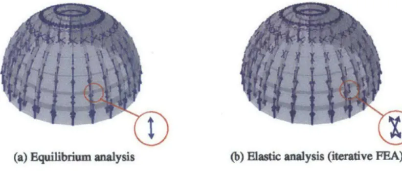
The equilibrium and elastic analysis use different physical models based on different approximations. Moreover, the objective function used in the equilibrium analysis (minimizing the sum squared forces) is rather arbitrary and not physically justified. Naturally, the solution found by the iterative FEA and the equilibrium analysis are usually different. Figure 15 compares the forces computed by the two methods in a dome structure. The equilibrium analysis outputs predominantly vertical forces at the bottom and hoop forces at the top. On the other

37

hand, the elastic analysis outputs larger hoop forces in all levels of the dome.

Figure 15: Both equilibrium and elastic methods find a compression-only solu-tion indicating that the structure is sta-ble. However, the two solutions are different. (a) The equilibrium analysis outputs predominantly vertical forces in the bottom of the structure, whereas (b) the elastic analysis outputs larger hoop forces.

(a) Equilibrium analysis (b) Elastic analysis (iterative FEA)

Future work

Resolving contact nodes do not solve the problem of indeterminacy in masonry. Consider a four-legged stool. It could be balanced by only two opposite legs, or equally by the four legs. In fact, there are infinitely many possible force configurations to make the stool stand and all of them are physically valid. Developing an efficient method to analyze hyper-static structures is an interesting challenge.

Further investigation is necessary to delineate the relationship between rigid body equilibrium analysis and elastic finite element analysis. The force formulation of equilibrium analysis and the displacement formu-lation of FEA resemble a primal-dual reformu-lationship. A unified frame-work to compare the two methods along these lines would be helpful. Efficient algorithms to handle contact and friction would significantly improve both methods. For instance, the safe theorem which states that if a compression-only equilibrium solution exists the structure is stable applies only to hinging failure under tension. For both equilib-rium and elastic analysis, how to efficiently compute friction and how to handle sliding are open questions.

Conclusions

This thesis explored computational and visualization tools to study the equilibrium of masonry structures. The following contributions are presented:

1. We extend the equilibrium formulation to determine the stability of masonry structures to include tensile elements such as cables. The quadratic formulation provides a measure of infeasibility, and the gradient of feasibility with respect to geometric modifications.

2. We apply the gradient of feasibility in the design of stable struc-tures. Starting from an unstable input model, we modify the geome-try to increase its stability while satisfying user-defined constraints. 3. We investigate various properties related to the equilibrium of a

structure and visualize the results.

4. We compare the equilibrium method to the finite element analysis (FEA). We point out the correct way to interpret tension in FEA, and explain the drawback of FEA that comes from formulating the contact constraints. We propose an iterative constraint relaxation approach to address this problem.

Bibliography

Philippe Block. Thrust Network Analysis: Exploring Three-dimensional

Equilibrium. PhD thesis, Massachusetts Institute of Technology, 2009.

Philippe Block and John Ochsendorf. Thrust network analysis: A new methodology for three-dimensional equilibrium. International

Association for Shell and Spatial Structures, 155:167, 2007.

Philippe Block, Matt Dejong, and John Ochsendorf. As hangs the flexible line: Equilibrium of masonry arches. Nexus Network Journal, 8(2):13-24, 2006.

Phillipe Block. Equilibrium systems: Studies in masonry structure. Master's thesis, Massachusetts Institute of Technology, 2005-C Dick,

J

Georgii, R Burgkart, and R Westermann. Stress tensor field visualization for implant planning in orthopedics. IEEE Transactions

on visualizations and computer graphics, 15(6):1399 - 1406, 2009.

ISSN 10772626. URL http://tibproxy.mit.edu/login?url=http:

//search.ebscohost.com/login.aspx?direct=true&db=edswsc&AN= 000270778900070&site=eds-live.

Carlos A Felippa and Ray W Clough. Thefinite element method in solid

mechanics. American Mathematical Society, 1970.

Roger Fletcher. Practical Methods of Optimization. John Wiley & Sons, Ltd, 1987.

Ran Gal, Olga Sorkine, Niloy

J.

Mitra, and Daniel Cohen-or. iwires: An analyze-and-edit approach to shape manipulation. ACM

SIG-GRAPH Trans. Graph, pages 1-10, 2009.

Jacques Heyman. The stone skeleton. International Journal of solids and

structures, 2(2):249-279, 1966.

Santiago Huerta. The analysis of masonry architecture: A his-torical approach. Architectural Science Review, 51(4):297-328, 2008.

DOI: 10.3763/asre.2008.5136. URL http: //www. tandfonline.com/ doi/abs/10.3763/asre.2008.5136.

42

Takeo Igarashi and John F. Hughes. A suggestive interface for 3d drawing. In Proceedings of the 14th Annual ACM

Symposium

on User Interface Software and Technology, UIST 'oi, pages 173-181,

New York, NY, USA, 2001. ACM. ISBN 1-58113-438-X. DOI:

10.1145/502348.502379. URL http: //doi. acm.

org/10.1145/502348.

502379.

T.R. Jagadeesh and M.A. Jayaram. Design of Bridge Structures, chap-ter 5. Prentice-Hall, 2000.

Olga Karpenko, Wilmot Li, Niloy Mitra, and Maneesh Agrawala. Exploded view diagrams of mathematical surfaces. IEEE

Transac-tions

on Visualization and Computer Graphics, 16(6):1311-1318, Novem-ber 2010. ISSN 1077-2626. DOI: 10.1109/TVCG.2010.151. URL

http://dx.doi.org/10.1109/TVCG.2010.151.

Danny M. Kaufman, Shinjiro Sueda, Doug L. James, and Dinesh K. Pai. Staggered projections for frictional contact in multibody sys-tems. ACM Transactions on Graphics (SIGGRAPH Asia 2008), 27(5):

164:1-164:11, 2008.

Robert S. Laramee, Christoph Garth, Helmut Doleisch, JAijrgen Schneider, Helwig Hauser, and Hans Hagen. Visual analysis and exploration of fluid flow in a cooling jacket. In In Proceedings IEEE

Visualization 2005, pages 623-630, 2005.

R. K. Livesley. Limit analysis of structures formed from rigid blocks.

International Journal for Numerical Methods in Engineering,

12(12):1853-1871, 1978. ISSN 1097-0207. DOI: 10.1002/nme.1620121207. URL http://dx.doi.org/10. 1002/nme. 1620121207.

Niloy

J.

Mitra, Yong-Liang Yang, Dong-Ming Yan, Wilmot Li, and Maneesh Agrawala. Illustrating how mechanical assemblies work. ACM Trans. Graph., 29(4):58:1-58:12, July 2010. ISSN 0730-0301.

DOI: 10.1145/1778765.1778795. URL http: //doi. acm. org/10. 1145/

1778765. 1778795.

Christopher Niederauer, Mike Houston, Maneesh Agrawala, and Greg Humphreys. Non-invasive interactive visualization of dynamic architectural environments. In Proceedings of the 2003 Symposium on

Interactive

3D Graphics, 13D '03, pages 55-58, New York, NY, USA,

2003. ACM. ISBN 1-58113-645-5. DOI: 10.1145/641480.641493. URL http://doi.acm.org/10.1145/641480.641493.

John Ochsendorf. Collapse of

masonry

structures. PhD thesis,

Univer-sity of Cambridge, 2002.

John Ochsendorf. Masonry arch on spreading supports. Structural