HAL Id: insu-02994631
https://hal-insu.archives-ouvertes.fr/insu-02994631
Submitted on 8 Nov 2020
HAL is a multi-disciplinary open access
archive for the deposit and dissemination of
sci-entific research documents, whether they are
pub-lished or not. The documents may come from
teaching and research institutions in France or
abroad, or from public or private research centers.
L’archive ouverte pluridisciplinaire HAL, est
destinée au dépôt et à la diffusion de documents
scientifiques de niveau recherche, publiés ou non,
émanant des établissements d’enseignement et de
recherche français ou étrangers, des laboratoires
publics ou privés.
Automatic determination of the electron density
measured by the relaxation sounder on board ISEE 1
Jean-Gabriel Trotignon, J. Etcheto, J.P. Thouvenin
To cite this version:
Jean-Gabriel Trotignon, J. Etcheto, J.P. Thouvenin. Automatic determination of the electron density
measured by the relaxation sounder on board ISEE 1. Journal of Geophysical Research Space Physics,
American Geophysical Union/Wiley, 1986, 91 (A4), pp.4302. �10.1029/JA091iA04p04302�.
�insu-02994631�
JOURNAL OF GEOPHYSICAL RESEARCH, VOL. 91, NO. A4, PAGES 4302-4320, APRIL 1, 1986
Automatic Determination of the Electron Density Measured
by the Relaxation Sounder on Board ISEE 1
J. G. TROTIGNON
Laboratoire de Physique et Chirnie de l'Environnernent, Orleans, France
J. ETCHETO
Centre de Recherche en Physique de l'Environnernent Terrestre et Plangtaire, Issy les Moulineaux, France
J.P. THOUVENIN
Centre National d'Etudes Spatiales, Toulouse, France
Relaxation sounders have proved to be successful in measuring the electron density in dilute space plasmas. The resonances excited at the characteristic frequencies of the medium depend very much on the local plasma. We present here methods to determine automatically, by a computer, the plasma frequency in the various regions encountered. In the solar wind and in the magnetosheath, only one strong,
long-lasting resonance appears close to the plasma frequency fpe, yielding directly the electron density.
We use a pattern recognition method based on Sebestyen's discrimination approach, and each identified resonance is given with a quality criterion. From one year of data there is no drift of the resonance
features,
and the method
• is used
with a success
rate of 95% as determined
by manual
means.
In the
magnetosphere various types of resonances are excited at the characteristic frequencies of the medium
(cyclotron harmonic frequencies nf• e and maximum frequencies of the Bernstein's modes fq,). We compare the dispersion relation of electrostatic waves, which contains fee and fpe as parameters, to the observed
frequencies of the resonances. First fee is extracted using the harmonicity of the nf½ e resonances, and then the fqn series is compared to the dispersion relation for various values off• e. In 93% of 250 cases the error for f•,e is less than 10%. In the magnetotail where the resonances are closely spaced in frequency, the frequency resolution of the experiment does not allow us to use this method and we determine f•,e by the enhancement of the resonances power.
1. INTRODUCTION
During the last twenty years the relaxation sounder was undoubtedly a part of the most used active experiments for the study of spatial plasmas. After proving to be successful in ionospheric dense plasma (see Calvert [1969], Muldrew [1972a, b], McAfee [1973], and Benson [1977] for reviews), it was taken aboard spacecraft flown in the dilute plasma of the outer magnetosphere: GEOS 1 (launched in May 1977), ISEE 1 (October 1977) and GEOS 2 (July 1978). Here again, the results obtained were of excellent quality [Etcheto and Petit, 1977; Etcheto and Bloch, 1978]. Finally it was on board ISEE
1 that such an experiment was used for the first time outside the magnetosphere and proved to work very well in the solar
wind and magnetosheath [Harvey et al., 1979].
The sounder transmits on a swept frequency and receives echoes after a measured delay in a way analogous to ground-
based ionosondes. The transmitter excites natural modes of
oscillation in the surrounding medium. Hence with suitable interpretation, we have a powerful tool for spatial plasma di- agnostic.
The aim of the present paper is to handle several years of ISEE 1 data using a computer and to determine automatically
a fundamental
parameter,
the plasma
frequency,
from the raw
data. This data processing
was essential
to change
the relax-
ation sounder into an instrument usable for routinely mea-
suring
the total electron
density
on board a spacecraft.
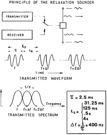
PRINCIPLE OF THE RELAXATION SOUNDER
I TRANSMITTER
RECEIVER f F+AF lIME f+2Af TRANSMITTED WAVEFORM . 1/•.fre
q
uenc_y_..
f f+Af f+ 2Af TRANSMITTED SPECTRUM '•' = 2.5 ms 31.25 ms125
ms
t$
=
1.5s
4s A f =1__=400 HzCopyright 1986 by the American Geophysical Union. Paper number 5A8595.
0148-0227/86/005A-8595505.00
43O2
TROTIGNON ET AL.' AUTOMATIC DETERMINATION OF DENSITY ON ISEE 1 4303 ISEE I December 8,1977 0322 26.5 kHz 80 40 0 0 waveform o 50 T(MS)
Fig. 2. Resonance in the solar wind. Top' envelope of the re- ceived signal in logarithmic scale. Bottom: compressed waveform. A resonance is a strong, monochromatic signal decreasing with time.
As a result of the eilipticity of the ISEE 1 orbite (aPogee 23
R e, perigee
280 km), the sounder
makes
measurements
in dif-
ferent plasma regimes (magnetosphere, magnetosheath, solar wind, magnetospheric tail) in which the signals have very dif-
ferent signatures. Consequently, we developed different meth-
ods to determine the plasma frequency, and thence the plasma
density,
in different
regions.
We will first describe briefly the principle of the relaxation
sounder
and the signals
observed
in different
regions.
In sec-
tions 3 and 4 we will detail the method used in the regions (magnetosheath and solar wind) where only one resonance is observed at the plasma frequency. Section 5 will deal with the determination of the plasma frequency in the magnetosphere,
where many resonances of different natures are observed.
2. RELAXATION SOUNDER: RESONANCES
The principle
of a relaxation
sounder
is similar
to that of fi
classical radar flown in a plasma (Figure 1). At the beginning
of a time interval
ts, a radio wave
transmitter
is co•hecte•l
to
an antenna
and sends
a wave
train with a center
frequency
f
and a durati
øn z. Immediately
after
this transmission
a radio
receiver tuned to the same frequency f is connected to the antenna; this receiver has a bandwidth Af = 1/z and listens tosignals
in the frequency
band
f + A
f/2 until
the '•nd
of the
time ts (frequency step). Then the frequency is incremented by
Af and the process is repeated at f + Af(new frequency step).
Let us notice that the receiver bandwidth A f of the topside sounders is much larger than 1/z. The reason is that the receiver of this type of sounder sweeps upward in frequency during the travel time of the pulse [Franklin and Maclean, 1969]. The ISEE 1 relaxation sounder has many possible
working modes chosen by telecommand [Harvey et al., 1978],
but the one most commonly used covers the frequency range from 0 to 51 kHz using 128 frequency steps, each of which is 400 Hz wide. The step duration ts is 125 ms, a complete cycle lasting thus 16 s. The received signal is compressed in an automatic gain control amplifier (AGC). The data are trans- mitted to the ground (1) either through a digital telemetry giving the AGC level, usually sampled once every 16 ms, which is used permanently (the plasma frequency determi- nation will be made on these signals) (2) or through an analog
telemetry,
used only 10% of the time, which transmits
both
the AGC level and the compressed waveform (these data will be used to help in the adjustment of the data processing).
If the transmitter is not used (passive mode), the sounder
becomes a natural wave receiver. The sounder is usually active
RESONANCES IN THE SOLAR WIND (1290) ( RAW VARIABLES ) -6 -18 I I I I , , I ' I I -1½ -lO
LOI3•o(POWER,
V z lm 2 Hz)
NON-RESONANCES (127800) -6 -18 -1/,LO[i•o
(POWER,
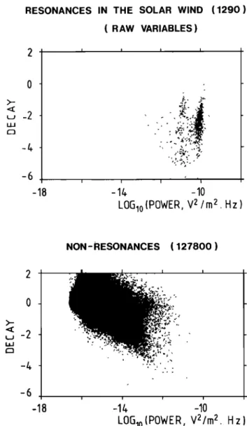
Fig. 3. Scatter plots of the raw variables in the solar wind for
I
-10
V2/m
2 . Hz)
resonances (top) and nonresonances (bottom). The scattering inside one family is larger and the decoupling between the two families is
4304 TROTIGNON ET AL.' AUTOMATIC DETERMINATION OF DENSITY ON ISEE 1
CHARACTERISTICS OF RESONANCES IN THE SOLAR WIND
( AUTOMATIC RECOGNITION ) 8OOO 6000 4000 2000 100 5O POWER -2
log
10
P ( arbitrary
units
)
1 2
ISEE
1
November 6 to
mi. 1977
, resononce s ( 690) non- resononces ( 86 000) DEVIATION TO MEAN DECAY0.
0.i5
8OOO 6OOO 4OOO 2000 100 5O 0 O.3O O.45 DECAY , T 1 -90 -50 -103'0
•0
Deviation ( arbitrary units ) Decay
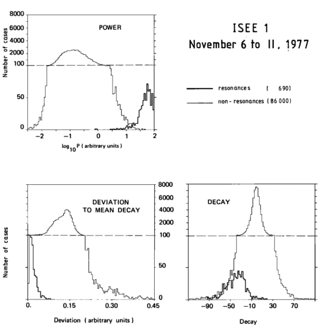
Fig. 4. Characteristics of resonances (thick line) and nonresonances (thin line) in the solar wind' "power" (top), "deviation" to mean decay (bottom left) and "decay" (bottom right). Resonances and nonresonances are well decoupled, especially for "power."
only part of the time, but in this paper we will deal only with data recorded during active periods.
The answer of the medium to the transmitted wave train, observed only at some frequencies, is called a resonance. Im- mediately after transmission, a very intense signal is observed, whose amplitude decreases slowly compared to the duration
of the transmission z: a resonance lasts approximately one hundred times more than the transmitted pulse. Such a phe-
nomenon can only be observed when the frequency of the
transmitted signal is close to a resonance frequency of the
medium at which the group velocity of the waves is low, be-
tween one and a few tens (depending on the type of resonance observed) of times the relative velocity of the satellite with
respect to the medium. In this case, the transmitted waves
travel with the spacecraft, or intercept its trajectory, in such a
way that the received signal lasts much longer than the initial pulse.
Detailed interpretations have been given for observations made in the ionosphere by Deering and Fejer [1965], McAfee [1969], and Fejer and Yu [1970]. For the sake of the present
study we will only mention that in the magnetosphere many resonances are observed' at the harmonics of the electron gy-
rofrequency,
at the fq, frequencies
of the Bernstein's
modes
of
propagation, at the upper hybrid frequency [Etcheto et al.,
1981]. It has been shown [Belmont, 1981] that in a bi-
Maxwellian
plasma
(made of a dominant
cold plus a hot
population)
there is a series
of fq, (one in each branch con-
TROTIGNON ET AL.: AUTOMATIC DETERMINATION OF DENSITY ON ISEE 1 4305
RESONANœES
IN THE SOLAR
WIND
(AUTOHATI[: REœOGNITION)
{690}
-50
•' 'Y,'
' 1
-1 30 !-2.5
-1 0
0'.5
2.0
POWER (arbifrary unifs)
• 0./•5 •- 0.30 z
_o 0.15
rn 0. -130 ß., .'.•½•.•':•.:.•a,•, -50 DECAY3b
11oNON- RESONANCES
IN
110 ' ' 30 -50THE SOLA R
0./,5
0.30- 0.15 0. -130WIND {86000}
i -130-2.5
-1'.0
O:S
2.0
-50
3'0
POWER
(ctrbi'l'rctry
unifs)
DE CAY
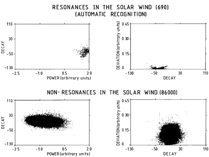
Fig. 5. Scatter plots of the variables for resonances (top) and nonresonances (bottom) in the solar wind. The decoupling
is even clearer in a three-dimensional space.
110
hybrid frequency) which only depend on the ratio of the plasma frequency of the coldest population to the gy- rofrequency and on the number of the branch in which they are observed. We will use this property later. Furthermore,
additional
fqn resonances,
called
"hot fqn,"
are observed
whose
number and frequencies depend on the characteristics of the
hot plasma. The intensity of the various resonances varies but
usually the strongest signal is observed close to the total
plasma frequency [Etcheto et al., 1983].
The data processing of the resonances in the magnetosphere will consist in determining the gyrofrequency (using the har- monicity of the gyroharmonics) and the cold plasma frequency
(through
the alignment
of the cold4n) [Trotignon
et al., 1982].
In the solar wind and magnetosheath where the electron tem- perature and the magnetic field are low, only one strong, long-
lasting resonance is observed close to the plasma frequency, even though an additional series of weak, short-lived reso-
nances at the gyroharmonics and f•tn is seen in the mag-
netosheath. In these regions, the data processing will consist in signal pattern recognition to identify the plasma resonance •Thouvenin and Trotignon, 1980], which is not more than one
or two percent off the plasma frequency as determined by
manual scaling of the data •Etcheto et al., 1981].
3. SOLAR WIND
A typical example of plasma resonance observed in the
solar wind is shown in Figure 2, transmitted through the
analog telemetry. At the top the AGC level is displayed as a function of time, the times of sampling of the digital telemetry being indicated. It is a strong signal, decreasing slowly with time. At the bottom, the compressed waveform (after fre-
quency transposition) is plotted: its amplitude evolves slightly
because the feedback is not total (the waveform is not com- pressed to a fixed amplitude but is only compressed from a 0- to 80-dB dynamic range to a 0- to 20-dB dynamic range). We will work on the digitized AGC signal, usually sampled 3 or 7 times during a given frequency step.
From now on, we will call resonances the frequency steps
where the observed signal behaves like a resonance, and non- resonances all the other steps. Our problem is now to separate the resonances from the nonresonances, automatically by using a computer, working on undersampled, possibly noisy signals, and keeping in mind that natural waves with com- parable intensity can be present simultaneously. This task is well performed using a pattern recognition technique. As the resonances have a common pattern, while the nonresonances can be anything (natural waves of various kinds, parasitic signals), we are only able to define the common features of the resonances. These features will characterize the class of reso- nances. Then we have to determine whether a given frequency
step belongs to the class of resonances or not by a comparison
of its features with the already known pattern of this class. Among the pattern recognition techniques, we have chosen Sebestyen's algorithm, which seemed to be the most suitable in
4306 TROTIGNON ET AL.: AUTOMATIC DETERMINATION OF DENSITY ON ISEE 1
ISEE 1 November6
11,1977
100 - 50- NQo N ... theoretical curve NRQ o NQo + NR Qo I I I I I 1. 2. 3. Quality criterion QoFig. 6. Percentages of signals having a quality better than a given
Q0 for resonances (thick line) and nonresonances (thin line). The
dotted line shows the theoretical results if the variables were normal.
N is the total number of resonances (N = 690). NQ0 (NRQ0) is the
number of resonances (nonresonances) with Q _< Q0. We must im-
prove the recognition.
our case (see Sebestyen [1962], Romeder [1973], and Thouve- nin and Trotignon [1980] for its application to this particular problem).
First we must find the common pattern of the resonances. Through a measurement process which is done on a reference set of resonances we obtain a set of numbers called variables
which best describe a resonance. Two "raw variables," named
"power" and "decay," may be used. The "power" is the maxi-
mum power of the signal on the frequency
step in (#V/m) 2
Hz-• without removing
the noise of the instrument,
and the
"decay" is the slope A of the signal assuming a time variation
of the form t A (the definition
of A is given in the appendix).
Figure 3, for which nearly 1300 frequency sweeps were used,
shows the scatter plots of the decay versus the decimal loga-
rithm of power for the resonances (top) and nonresonances (bottom). Note that the average decay of the resonances is close to the value -2.35 given by Etcheto et al. [1981] using
the analog telemetry.
The set of points representing the resonances does not satis- factorily cluster in the sense that the "distances" between the points are not small enough, on average. Moreover the cluster of resonances is not well separated from the cluster of nonres-
onances. The fingerlike structure and spread of the clusters originate from the various modes in which the experiment was
working (different sampling rates and times, change of the
time constant of the AGC). It is worth noticing that the non- resonances decay with time. This is the result of a spurious signal, due to the transmitter, observed at the beginning of each step; the stronger the interference, the larger the decay, giving a slope to the cluster of the nonresonances. These are the reasons why we had to use the more sophisticated vari- ables described in the appendix.
Using these three variables called "power," "decay" and "de- viation" we will consider that the resonances are represented geometrically as points in a three-dimensional space. The first task of Sebestyen's algorithm is then to transform this original
space in order to increase the clustering of these points. In the
new space
the mean-square
distance
D: between
the members
of the reference set of resonances is minimum (for more details see Sebestyen [1962]). In Figure 4 are shown the histograms of the new variables which are obtained after having done the
transformations which minimize D 2. For the reference set of
resonances that we used, the cluster is only rotated through an angle of nearly three degrees about the deviation axis. There- fore the original variables (defined in the appendix) are very nearly independent. These histograms are made out of 690 frequency sweeps (containing 690 resonances and 690 x 128- 88,320 steps). We excluded the known parasitic lines at 20 and 40 kHz [Harvey et al., 1979] which are usually as strong as the resonances but without any decay. The histo- gram for the resonances is a thick line while it is a thin line for the nonresonances. The horizontal dashed line indicated the change from an enlarged linear scale to a more compressed one. The power is by far the most discriminating variable, followed by the "deviation." The decay comes last. Tests made when sorting the resonances by frequency bands did not show appreciable modifications.
We displayed the variables separately but the computer will handle them simultaneously and work in a three-dimensional
space, which representation is difficult. Thence we will project
the two clusters (of resonances and nonresonances) on the
planes orthogonal to the axes. The scatter plots in the "decay-
power" (left) and "deviation-decay" (right) planes are shown in Figure 5 for the resonances (top) and nonresonances (bottom).
This time the resonances cluster well, and the cluster of reso-
nances (less than 1% of the observed signals) is well separated from the cluster of nonresonances: the chosen variables de- scribe properly the resonances, and the discrimination is satis- factory.
Keeping in mind that the problem of finding the common pattern of the resonances is tackled by performing the trans- formations of the initial space which will cluster most highly the resonances in the new space, we can say that the calcula-
tion of D '• is a mathematical way to express this common
pattern.
We are now dealing with the second task of Sebestyen's algorithm, called the decision making process. We want to know whether a given frequency step A belongs to the class of
resonances or not. We must compute S(A) the similarity of
this signal to the signals of the class of resonances (here simi-
larity means closeness in the new space). S(A) is the mean-
square distance between A and the class at resonances repre- sented by the set of points in the new space. For each fre- quency step that we wish to sort out we will calculate the normalized coefficient Q(A)= S(A)/D • which measures the quality of the signal pattern recognition: the smaller it is, the more likely is A to be a resonance. This quality coefficient varies within the range (0.5, + c•). When the number of reso-
TROTIGNON ET AL.' AUTOMATIC DETERMINATION OF DENSITY ON ISEE 1 4307
lOO
ISEE 1
November
6 to II, 1977
Recognized resonances
without Qmin criterion
with Qmin criterion
0.5
false resonances
I I i I '1 I
1 1.5 2
Quality criterion Qo
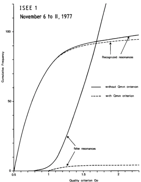
Fig. 7. Percentages of recognized resonances and false resona•ces versus Q0 when taking all the signals with Q _< Q0 (solid line) and when taking only the signal with the best quality (Qmin • Q0) in each sweep (dashed line). This latest test does not change much the number of recognized resonances but decreases drastically the number of false resonances.
nances of the reference set tends to infinity, the lower bound is
reached at the gravity center of the class of resonances, and the average value of Q for the set of resonances is 1.
We will now discuss some results. Let us consider N fre-
quency sweeps in which we have identified the resonances by a manual process. Each sweep is made of K frequency steps and only one is a resonance. For each step of the N x K steps under study we calculate its Q quality coefficient, and then for
a given threshold
Qo we look for the Moo steps
having
Q <
Qo. Among
these
Moo steps,
Noo are really resonances
while
NRoo
are nonresonances
(Moo
= NRoo
+ Noo).
The results
of
this process are plotted in Figure 6. The percentage Noo/N oftrue resonances satisfying Q < Qo is drawn against Qo with a thick line. For comparison we have plotted in dotted line the theoretical curve under the assumption of normal variables. Moreover, to evaluate the pollution rate of the recognition
process,
the percentage
NRoo/Moo of nonresonances
with
Q -< Qo against Qo is shown by a thin line. Among the steps with Q <_ 1.3, 78% are resonances (which represent 86% of the
resonances of the reference set) and 22% nonresonances. For a threshold of 1.7, 92% of the resonances are recognized but an
equal number of nonresonances are taken with them, while for Q < 1 there is a 3% pollution but only 70% of the resonances
are recognized.
If we now assume there is, at most, one resonance per fre-
quency
sweep,
we can improve
considerably
the results.
Of
course,
when the plasma frequency
is out of the range of the
sounder
(obviously,
there is no such case
in the reference
set),
the program
will give a false
resonance.
Fortunately
this "res-
onance"
will usually
have a bad quality coefficient
and will be
rejected
through using an adequate
threshold
value of Q.
Moreover we do not take into account the case when the
plasma frequency
varies at a rate comparable
with the fre-
quency sweep and is observed several times. Therefore, in each
frequency sweep we look for the step in which Q is minimum
and retain it as the most probable resonance. The results are shown in Figure 7 where the percentages of recognized reso-
nances and false resonances having Q <_ Qo are shown versus
Qo, by dashed
lines
when using
this Qmin
criterion
and by solid
lines when not using this criterion. Since all these percentages
are evaluated with respect to the total number N of reso-
nances which are expected, we can meet percentages of non-
resonances
NRoo/N greater
than 100% when not using
the
Qmin
criterion
(the nonresonances
are more numerous
than the
resonances). When using the Qmin criterion a few resonances
are lost (1% for Qo = 1.7 and 3% for Qo = 2.3) but the per-
centage of nonresonances
is drastically
decreased
(zero for
4308 TROTIGNON ET AL.' AUTOMATIC DETERMINATION OF DENSITY ON ISEE 1
RESONANCES IN THE MAGNETOSHEATH (1195)
{ RAW VARIABLES) >- •-2 -4 -6 -18 ! 1 -14 -10
LOI3•o
(POWER,
V
2/m
2.
Hz)
NON-RESONANCES (130600) Fig. 8. -2 -4 -6 -18 -14 -10LOI3.•o
(POWE
R, V
2/m
2 . Hz)
Same as Figure 3, in the magnetosheath. The results are
similar.
In summary, the steps with the minimum Q value in each sweep will be 95% of the resonances and less than 5% of nonresonances when Q < 2.5. Depending on the way the re- sults will be used, a threshold can be put on the Qmin: for a
low Q0 some resonances will be missing but the recognized
ones will not be polluted (that means, for a few sweeps there will be no recognized resonances). The accuracy of the plasma frequency determination is on the order of 400 Hz (one fre- quency step), that is, 4% for the density when the plasma frequency is 20 kHz. These results were corroborated by one year of data in the solar wind without any significant devi- ation of the characteristics of resonances with time.
4. MAGNETOSHEATH
In this region, as in the solar wind, only one strong, long- lasting resonance is observed at a frequency close to the plasma frequency. At frequencies above the plasma frequency, additional, weak, short-lived resonances are observed at the harmonics of the electron gyrofrequency [Etcheto et al., 1981]. Since the gyrofrequency is on the order of 500 Hz, these reso- nances are properly observed only using the analog telemetry and will be ignored, so that we will consider that only one resonance is observed at the plasma frequency.
The scatter plots of the decay versus power (raw variables)
are shown in Figure 8 for resonances (top) and nonresonances (bottom) from about 1200 frequency sweeps recorded from December 29, 1977, to January 25, 1978. This figure should be compared to Figure 3 on which are displayed the same vari- ables in the solar wind. The plots for the resonances are very similar, and the same signals pattern recognition method should be applicable. More precise comparisons made on the
three variables power, decay and deviation showed no signifi-
cant difference between plasma resonances in the solar wind and those in the magnetosheath. As a matter of fact, when Sebestyen's algorithm is used on the magnetosheath data, we obtain the same percentage of success using the solar wind reference set or the magnetosheath one.
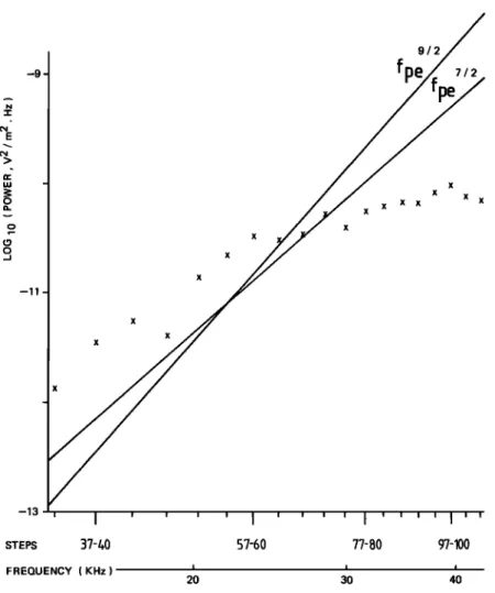
At last we should point out a tendency for the power of the resonances to increase with frequency, as can be seen in Figure 9. Here the average power is plotted against frequency (raw variables) by bins of four steps, for both magnetosheath and solar wind resonance sets together. This is in line with the theoretical results of Deering and Fejer [1965] and Fejer and
Yu [1970] which predict a variation proportional
to f9/2 for
signals accompanying
the satellite or to f?/2 for oblique
echoes. These two laws are shown as solid lines in Figure 9 but the frequency range covered is too small and the receiver saturation level too low to decide between them.
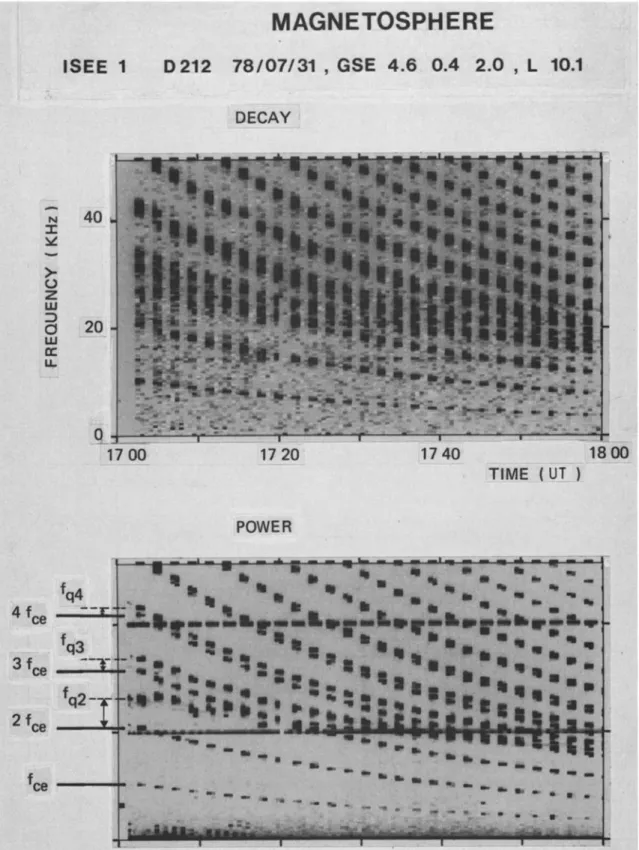
We will now look at the results given by this program for a case of multiple bow shock crossings. Figure 10 shows a dy- namic spectrogram of the sounder data for a three-hour period during which the earth bow shock was crossed several
times. The frequency scale is linear between 0 and 51 kHz
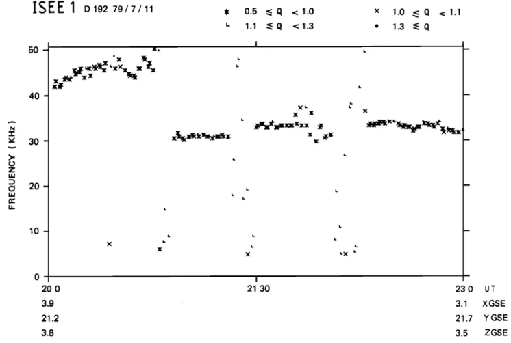
while the grey scaling depends on the strength of the received signals. The tick marks at the top of the frame indicate the times when the sounder was active. At the beginning of the period the spacecraft is in the magnetosheath, and the plasma frequency varies between 40 and 51 kHz, going out of the range of the sounder at 2048 UT. The satellite enters the solar wind at 2054, and the plasma frequency stays around 30 kHz until 2120 when the spacecraft crosses the bow shock again. In the magnetosheath, between 2120 and 2130 the plasma fre- quency is out of range. When the spacecraft enters the solar wind again at 2130, the plasma frequency is 33 kHz. From 2148 to 2154 a burst of upstream natural noise [Etcheto and Faucheux, 1984] is observed. The satellite makes a new excur- sion into the magnetosheath, where the plasma frequency is above 51 kHz, from 2205 to 2218 and from then on stays in the solar wind. The program for automatic resonance recogni- tion was run on these data, and the results are shown in Figure 11. The frequency of the recognized resonance when using the Q minimum criterion is plotted as a function of time, using a symbol which depends on its quality: an asterisk for Q less than 1, a cross between 1.0 and 1.1, an L from 1.1 to 1.3 and a circle above 1.3. As we kept one resonance per sweep, there is a result even when the plasma frequency is out of range, but during these periods the quality is poor (hardly an asterisk), and if we had put a threshold on Q we would have kept only true resonances. For this day, we had only three AGC samples per step.
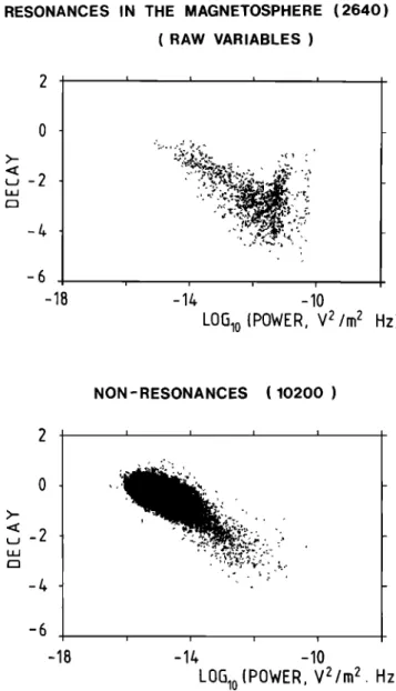
5. MAGNETOSPHERE
In the magnetosphere, contrary to what is observed in the
solar wind, many resonances of different nature are observed, and the problem is no longer to distinguish a resonance
among nonresonances but to name the different resonances
and deduce the plasma frequency. An example is shown in Figure 12 where the decay (top) and power (bottom) com- puted as raw variables on each of the 128 frequency steps are
TROTIGNON ET AL.' AUTOMATIC DETERMINATION OF DENSITY ON ISEE 1 4309 9/2 -11
-9
f
7/2
x x x x x x x x STEPS 37%0 57-60 77-80 97-100FREQUENCY
(KHz)
20
Fig. 9. Average power as a function of frequency for resonances in solar wind and magnetosheath. The power increases with frequency.
shown on a frequency versus time display, the grey scaling depending on the value of the parameter. During this period the satellite was at high magnetic latitude (50ø), its geocentric distance varying from 5 to 7 Re near noon. Two series of resonances due to propagation of the waves on the Bernstein's modes [Bernstein, 1958] are seen: the gyroharmonics nfce and
the fqn
frequencies.
5.1. Pattern Recognition Study
The power and decay of the resonances are much more variable in the magnetosphere than in the solar wind. This can be checked in Figure 13 (which should be compared to Figure 3) in which the scatter plot of decay against power is shown for the resonances (top) and nonresonances (bottom) for a hundred sweeps recorded between November 29, 1977, and December 14, 1977. The two clusters are not far apart enough to allow for a proper discrimination. The reason is that many
weak and short resonances resemble nonresonances and also
that strong resonances give images on the adjacent steps,
which are nevertheless considered as nonresonances.
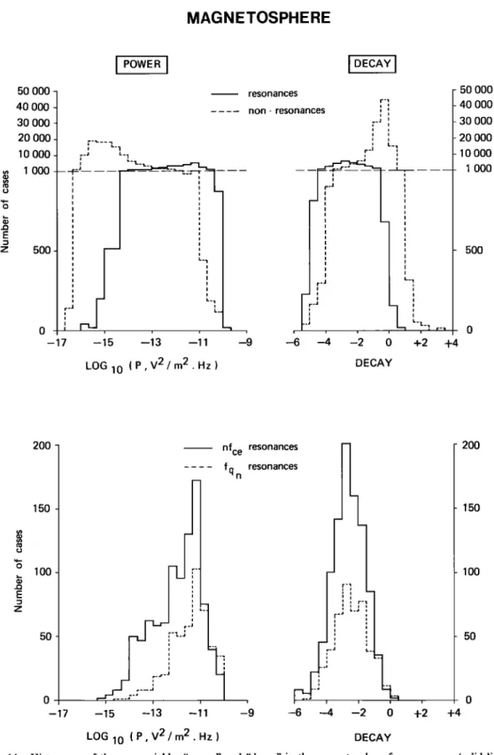
The next question is, is it possible tO sort out the various
types of resonances using the raw variables power and decay?
The bottom panels in Figure 14 show that the answer is again
no. In this figure are plotted
the power (left) and decay
(right)
for the resonances and nonresonances (tOp) and for the two
types of resonances
(bottom).
The top papels
confirm what is
seen in Figure 13: the resonances and nonresonances are not
sufficiently
discriminated.
In addition,
we do not know
in ad-
vance the number N of resonances excited during one sweep, and it is not possible to select for instance the N resonances having the best quality, a method which we have seen to be very efficient in the solar wind.
Therefore, in the magnetosphere the signal pattern recogni-
tion methods • are not likely to give very good results, either to
discriminate between resonances and nonresonances or to identify the different families of resonances. To quantitatively support these conclusions we have to show a comparison of the results obtained in the solar wind and in the mag- netosphere by using a simple threshold criterion: P > Po and D _< Do, where the power P and the decay D are the raw variables defined in section 3. In Figure 15 we have plotted the percentage of resonances having P _> Po and D _< Do against the percentage of nonresonances satisfying the same criterion: for a given Po while D O is varying (solid lines) and for a fixed Do and Po varying (dashed lines). Note that those curves are respectively labeled in log Po and in Do. Moreover, the per- centages are computed with respect to the total number of resonances which are contained in each data set (solar wind in the top frame or magnetosph9re in the bottom frame). A data set means a group of sweeps in which we have identified all
the resonances with a manual process. In these data sets the
nonresonanc6s are more numerous than the resonances, so for
low values
of Po and
larg
e values
of D O we can
have
more
4310 TROTIGNON ET AL.' AUTOMATIC DETERMINATION OF DENSITY ON ISEE 1
:- .•.::•
'• •' •'" • I •-:'=}. ...
:"•'".,,,-.
...
...
•.,-' I:
... •'-• ... ..•':': ... :.:..:. ... ..r•. • ..•'. ?:;;:.•; :•.. ?•;:;•c TM'•:•:•: •..::•-.:•.•. :..-...•-•.••.•.::- •: •:•,• ...;•;.•? ... . .__.-.•.•;• ... .. t ... m ?-•: .... ::- .'.:;<•: ... •,• /"7" '?-;'•':+"•"•-i •' .•.•,•;:-:-t'¾....•,•'.'_.'.'? i' •'"'"'•-•:• ;•.' .'•.•.<•;;•: :.&.-.;.-- •'v'"7 :;;?• '";'t..'"•'t ... ?•'"•:•:L ....: ... ?;?::: •:.:.:•-:-• -s;;•. -.•: --:•½m?c:h•:•.;;"-'. '- ' -:m%•::m•:•A•-:-• • .... •:: Y• •::•:•'"'•:•'•'•.•:•c• ...•..?-' -. •....::•;;:•
:•..:•'•
...
•'•U'•,••'•
:,..
•'•'-•
'•$":•
'• '"f•'
:•
.-:"•
ß ' - ... '--"- .•:,..- ... - '• . :. ;½ ... . ... ':•::• .... •.. •c•--::- :?•?•::'½g{-:•-{• .•;:-•- -• -• •.. • ;•)' r •;:. :- :.. . ..?...:::::•..::..?. ß : ... .:.. :. ... . ..::..• =... ... ,,.. ,,, . ,,:... ,...:..._....• ...: _.... . .... •..._...:-....:-•?• •,,-
•.•.•.•.
= ....
7 •?':•
:'%:"'2
"•"::•'
...
• • ...r'y• ... • •:• "•'•: ' .... • . ... • :;? •L"" ?:•.:•?•:•-.:':-" ' .,., . ':?:'-:-AY•'•:• '?:""•;:-•:.•:•'•'• •. '•. .• .• ... ';"7'....,. .... :.•:•:•' •;•" r'... • .,•.. ....'•.•:". ..., ... iV....•$' .... •' •:• :•;• ... •;• ....-•: . :,?•? .... •;•'s•' t.•:•:•;)•::•h• ... • ,'- -,: •:r¾-:: ... •:'-'• - - - = •':. ' ' ' :..:• ... - .•,'"'..•...,'•;...•. : ... •'" ?:.. - 0 ?• ... :• ... :"- • ... -?="•:-•:-: -• ... ' ... '_ •:.? "•77" .'•:.?•<";;•'• •. .... = .. •.• "'1' '"•" ... •;-'•:• ...TROTIGNON ET AL.' AUTOMATIC DETERMINATION OF DENSITY ON ISEE 1 4311 50- 40- 30- 20- 10- , 0.5 .< Cl < 1.0 x ' 1.1 -< 0 <1.3 ß I X 6
•Xa•xX•Xxxx •
1.o 1.3 <1.1 t_ X '..X 2O 0 21 3O 23 0 3.9 3.1 21.2 21.7 3.8 3.5Fig. 11. Results of the automatic data reduction for the same period as in Figure 10. When the plasma frequency is out
of the frequency range of the experiment, the quality of the most probable (false) resonance is bad.
UT XGSE
YGSE ZGSE
number of resonances we are looking for. This is the reason why the percentage of nonresonances (PNR) can be greater than 100%. To know the percentage of recognized resonances for given P0 and Do thresholds one should consider the inter- section of the relevant power and decay curves. Suppose that we have to sort out 100 resonances. If we accept a pollution of 20% by nonresonances (PNR = 20), that is, if we do not
accept more than 20 nonresonances among the recognized signals, we will not recognize more than 75 resonances
(PR -- 75) in the solar wind (which corresponds approximately
to log Po = -11.75 and Do = -1.8) and 65 (PR = 65) in the magnetosphere (log Po = -12.5, D O -- --1.). If we allow only
for 10% pollution, we will recognize 72 resonances in the solar wind and only 45 in the magnetosphere. Moreover, in the magnetosphere the average number of resonances per sweep is 30. So, if we accept a 20% pollution, we will obtain 30 x 0.65 -- 19.5 good resonances and 30 x 0.2 --6 wrong resonances per sweep instead of the 30 good resonances we were looking for. This is the reason why this recognition method (even improved by using Sebestyen's algorithm) is not usable in the magnetosphere and we will then rely on the physical knowledge that we have of the phenomenon.
5.2. Use of Dispersion Relation of Bernstein's Modes
Figure 16 shows the received amplitude (the average of the electric field) on the ordinate (after subtracting the noise of the
experiment) as a function of frequency. In this display the
resonances appear as peaks.
The most easily identified are the gyroharmonics, due to their harmonicity. We use the measurement of the on-board magnetometer as an initial value and compare the data to the series of resonances, computed in frequency steps for several gyrofrequencies taken close to this initial value. This pro- cessing is applied after removing from the signal the slow variation of the amplitude with frequency, which is determined in the way explained below. The best fit gives the gy- rofrequency with an accuracy of 0.7% (the modulus of the magnetic field is known within less than 1 7 in a 100-7 field).
We can now determine
the f•. resonances
and the plasma
frequency
f•,e. We have seen
that in a Maxwellian
plasma
the
f•. normalized
to the gyrofrequency
only depend on the
plasma frequency (normalized to the gyrofrequency too). We
use the dispersion relation, stored in the computer, to deduce
series
of theoretical
f•.for various
values
of f•,e.
We then com-
pute the frequency of these theoretical resonances using the
gyrofrequency
that we have
just determined.
Each
f•.series is
then compared to the observed signals, and weighted in order
to favor the lowest-order
f•. The f•.series which
best fits the
observations
gives
at the same
time the theoretical
f•. and the
plasma frequency. If the plasma is not Maxwellian, it will be the plasma frequency of the coldest component. But, in order to minimize the computing time of this correlation, we need a
reasonable initial value. We have established from many ob-
4312 TROTIGNON ET AL.' AUTOMATIC DETERMINATION OF DENSITY ON ISEE 1
Fig. 12. Dynamic spectrogram of the raw variables, "decay" (top) and "power" (bottom) for an outbound pdss in the magnetosphere. Many resonances are observed.
intense close, and above, the plasma frequency (a detailed study of one case observed on GEOS 2 is made by Etcheto et al. [1983]). We therefore smoothed the spectrum shown in Figure 16, obtaining the dotted curve, which frequency of
maximum amplitude was used as the initial value of the plasma frequency. The smoothing is obtained by computing
the fast Fourier transform of the signal made of the 128 values
measured in one sweep and filtering this spectrum by multi- plying by [1 •- cos (rcJ/10)]/2 the ten lowest-frequency compo- nents (J = 0, 1, .--, 9) and by 0 the higher-frequency compo- nents. This filtered spectrum then undergoes the inverse fast Fourier transform, resulting in the dotted curve of Figure 16.
TROTIGNON ET AL.' AUTOMATIC DETERMINATION OF DENSITY ON ISEE 1 4313
RESONANCES IN THE MAGNETOSPHERE (2640) ( RAW VARIABLES ) -6 -18 i i i i i i i i -1/+ -lO
L06•o
[POWER,
V 2/m
z. Hz)
NON-RESONANCES (10200 ) -6 -18 o- ,- . .:;.' :... -, I I I -1/+ -lOLO•o{POWER,
V z/m
z Hz)
Fig. 13. Same as Figures 3 and 8 in the magnetosphere. The reso- nances represent now 20% of the signals and are no longer clearly
decoupled from nonresonances.
Above the curves of Figure 16 is shown the result of the
identification of the resonances. At the top the results of the manual identification (using the analog telemetry) are gy-
roharmonics,
fan, and f,,, which does not belong
to these
two
families. Below, the results of the automatic analysis are as
described
above.
The gyroharmonics
and
fan
are correctly
rec-
ognized
(with
400-Hz
accuracy).
The plasma
frequency
fpe
de-
duced
from the fan resonances
does
not correspond
to a reso-
nance and is shown above 3fc e by a thick arrow.
In order to discuss in more detail this method for determin-
ing the plasma
frequency,
using
the
fan
resonances,
we will use
Hamelin's diagram shown in Figure 17 [Hamelin, 1980; De Feraudy and Hamelin, 1978]. All the frequencies are normal- ized to the gyrofrequency fce' Each curve labeled n is the locusof a given
fan when the plasma
frequency
varies.-On
the ordi-
nate is plotted
the deviation
in frequency
between
this
fan
and
the gyrofrequency just below (of order n) versus the plasma frequency (plotted on the abscissa). For a given plasma fre-quency
fpe, all the f•n are aligned
on a vertical
line, provided
the plasma is Maxwellian.
If we identify an fan resonance,
knowing the gyrofrequency, we can mark it on this diagram. If
several
fan resonances
are on a vertical
line, we can conclude
that the plasma is close to Maxwellian and deduce the plasma
frequency.
On the left part of Figure 17 we have plotted with horizon- tal lines the results of the manual identification using the
analog telemetry (8-Hz frequency resolution) and with thick lines the results obtained using the digital telemetry (400-Hz frequency resolution). The plasma frequency determined by the computer from the digital telemetry is shown by an arrow.
Using the analog telemetry,
each
fan resonance
(except
f•3) is
split into two, but the agreement between the automatic deter- mination of the plasma frequency and the manual determi- nation is good, even when the analog telemetry is used.
On the right-hand side of Figure 17, another example is
shown,
in which
the splitting
of the f•n resonances
is larger
and
the alignment less clear. Nevertheless the automatic recogni-
tion of the f•n resonances
from the digital telemetry
(thick
lines) is still correct. Belmont [1981] has shown that in a non-
Maxwellian
plasma
the fan frequencies
could be split and not
aligned, corresponding to plasma frequencies ranging from the
plasma frequency of the coldest component to the total plasma frequency. For a bi-Maxwellian plasma (a cool and a hot component), this range of apparent plasma frequencies is
larger when the two populations are more decoupled. The
splitting
of the f•n that we usually
observe
on board ISEE 1 is
of the type foreseen by the theory for two populations whose temperatures are not very different but whose densities differ significantly.
The program of automatic determination of the plasma fre- quency works on the digital telemetry and cannot see the
splitting
of the fan resonances,
owing to the lack of frequency
resolution. It fits first the gyroharmonics (obtaining an average value when the gyrofrequency varies during the fre- quency sweep) and then uses this value of the gyrofrequency
to compute the frequencies of the theoretical fan resonances
and fit them to the observations. The accuracy of this gy-
rofrequency
has a strong
influence
on the fit of the fan as can
be seen on the inset in the center of Figure 17. A theoretical
series
of fan lying on the vertical
line at fpe/fce
= 4.4 has been
replotted on the Hamelin's diagram after normalizing it to
1.007
fce (left series)
and to 0.993
fce (right series).
The fan are
now clearly misaligned, more for larger n, to the left if the gyrofrequency is increased, to the right if it is decreased. This misalignment is still tolerable by the computer owing to the poor frequency resolution of the digital telemetry. A larger
error for fce would change
the frequency
of the first fan by a
quantity exceeding the frequency resolution of the experiment and is therefore not tolerable.
On the two Hamelin's diagrams of Figure 17 an additional resonance labeled f,, (plotted with an asterisk) is observed be- tween 3 and 4 fce in the left-hand diagram and between 4 and 5 in the right-hand one. It is likely [Belmont, 1981] that this resonance is close to the total plasma frequency while the
alignment
of the f•n resonances
corresponds
to the plasma
frequency of the coldest population. One should notice that to
look for the f•n resonance
of lowest frequency
and consider
that the plasma frequency lies between this frequency and the gyroharmonic just below it, is risky. It assumes that it is possi-
ble to determine
the first fan, which is not necessarily
true,
especially when it is between a critical value, on the order of
(r• + 0.7)fce , and (n + 1)fce , a region in which the damping is
very strong when the propagation is not strictly perpendicular
4314 TROTIGNON ET AL.' AUTOMATIC DETERMINATION OF DENSITY ON ISEE 1
MAGNETOSPHERE
50 000- 4O 000 - 30 000 20 000 10 000 1 000 500 i ! i ! ! ! ! ! ! ! • L-' I i 'I'"
-
'1--
'l-
-.•
•.•
I L-. t ,, i i i i -15 --13 --11LOG
10 ( P ' V2
/ m2'
Hz
)
resonances non - resonances -50 000 -4O 000 -30 000 20 000 10 000 1 000 5OO DECAY 200 150 100 E z 5O o -17 nfce resonancesf q resonances
n •.., ',i r-J
•-J•J• r- --•"' i
i
--15 -13 -11 -9LOG
10 ( P, V2
/ m2' H7
)
I I I -2 0 +2 +4 200 150 100 5O DECAYFig. 14. Histograms of the raw variables "power" and "decay" in the magnetosphere for resonances (solid line) and
nonresonances (dashed line) at the top and for gyroresonances (solid line) and f•,resonances (dashed line) at the bottom.
The resonances are no longer decoupled from the nonresonances, and the different families of resonances have the same characteristics: the signal pattern recognition method has to be abandoned.
the technique
of alignment
of the f•n compared
to this latest
method
is to use the whole set of f•n, thus providing
a neces-
sary cross-check.
Out of 250 frequency sweeps that we studied carefully, the accuracy of the plasma frequency deduced by the computer
from theft. resonances
is better
than 10% in 93% of the cases.
In 96% of the cases this frequency (which is close to the plasma frequency of the coldest population) is less than 10% lower than f,, (which is close to the total plasma frequency). On the other hand, the frequency of the maximum of the
TROTIGNON ET AL.' AUTOMATIC DETERMINATION OF DENSITY ON ISEE 1 4315 smoothed spectrum (used as an initial value for the plasma
frequency determination) is above f,, in 97% of the cases. For 60% of the sweeps this maximum is less than 10% above f,,, and in 96% it is less than 20% above f,,. Usually this maxi-
mum is between
the first and the second
fq,, and closer
to the
second one.
Figure 18 shows the dynamic spectrogram of the sounder data (continuously active), for an example of density fluctu- ations observed on January 13, 1982, between 1810 and 1910 UT, while ISEE 1 was leaving the plasmasphere. At low fre- quency only resonances at the gyroharmonics are observed.
Above,
the f•, are superimposed
on the gyroharmonics,
giving
the impression of a darker region, whose lower edge corre- sponds to the plasma frequency. The results of the program of automatic determination of the plasma frequency are plotted as a function of time in Figure 19. In the top frame, the solid
line is the density
deduced
from the alignment
of the f• while
the dashed line represents the time evolution of the maximum of the smoothed spectrum. This latest curve is always above the density curve and follows the density fluctuations. In the bottom frame is displayed the modulus of the magnetic field after a rough detrending, obtained by substracting a mean magnetic field approximated by a polynomial of third degree. This rough processing is sufficient to evidence the compres- sional character of these Pc 5 pulsations. Even though the density is undersampled and the magnetic field averaged, the pulsations are in phase on both quantities (particularly at the beginning), as in the case studied by Kivelson et al. [1984] of a pulsation with a similar period of 7 minutes, but at a com- pletely different local time (near noon). This pulsation is a quiet time event (Kp _• 1 + during the previous 24 hours). Singer et al. [1979] studied Pc 3, 4 and 5 in the morning sector using simultaneous measurements on board several sat- ellites, but their density measurements were not sampled fast enough to evidence fluctuations. Between 1815 and 1830, superimposed on the pulsations, a density increase is observed simultaneously with a decrease of the modulus of the.magnetic field, without any particular change in the direction of the magnetic field. This short-lived density increase could be due to a plasma cloud. If we assume that the total pressure (kinetic plus magnetic) is constant from 1810 to 1830, the proton per- pendicular temperature is estimated to be on the order of 70
eV.
In the magnetospheric tail, the resonances are weaker and shorter than in the inner magnetosphere. They are also more closely spaced in frequency (typically 1 kHz or less). Even in this case the magnetospheric version of the program of auto- matic determination of the plasma frequency gives satisfactory results. When the gyrofrequency is too low to be resolved by the experiment, an estimate of the plasma frequency is given by the frequency of maximum intensity of the smoothed spec- trum. This method has been used by Etcheto and Saint-Marc [1985] to study the plasma sheet boundary layer.
6. SUMMARY AND CONCLUSIONS
The relaxation sounder, even though it has been widely used in passive mode to study waves spontaneously generated by the plasma [Christiansen et al., 1978a, b; Etcheto et al., 1982; Etcheto and Faucheux, 1984; Lacornbe et al., 1985], is primarily an active experiment, aimed at exciting radio waves at the characteristic frequencies of the medium, thus bringing information on the local plasma. The most interesting of this
information is a reliable and accurate determination of the
electron density. In order to make the instrument easily usable for routinely measuring the electron density it was necessary
lOO • 5o Non-resonances, percent (PNR) 100 -
log
Po
=-14_._..__••
MAGNETOSPHERE POWER Po DECAY D O Do =F'•I Non-resonances, percent (PNR)Fig. 15. Percentages of resonances (ordinate) and nonresonances (abscissa) having a power larger than Po and a decay smaller than D O in the solar wind (top) and magnetosphere (bottom). While in the solar wind a simple threshold on the "power" and "decay" enables us to roughly sort out most of the resonances, this is no longer true in the magnetosphere.
to develop an automatic method for determining the plasma frequency, working in any region visited by the satellite. We realized this tool for the relaxation sounder flown on board
ISEE 1.
In the solar wind and magnetosheath, where only one strong and long-lasting resonance is observed close to the plasma frequency, we used a signal pattern recognition method, the quadratic discrimination of Sebestyen [1962]. Each recognized resonance has a quality coefficient enabling the user to sort out the results according to the use he wants to make of them. A proper sorting enables us to recognize more than 95% of the resonances, thus determining the den- sity with an accuracy of 4% for a 20-kHz plasma frequency.
In the magnetosphere where many resonances are observed, such a method is no longer usable since the signal pattern between various resonances is more different than it is be- tween a resonance and a nonresonance. We therefore compare the observations to the theoretical dispersion relation of the Bernstein's modes. The electron gyrofrequency is determined with an accuracy better than 0.7%. The plasma frequency of the coldest population is determined with an accuracy better than 10% in 93% of the cases while the total plasma fre- quency is given within 10%. A direct check of these results cannot be made since no experiment is able to give the total