HAL Id: hal-01604267
https://hal.archives-ouvertes.fr/hal-01604267
Submitted on 28 May 2021HAL is a multi-disciplinary open access archive for the deposit and dissemination of sci-entific research documents, whether they are pub-lished or not. The documents may come from teaching and research institutions in France or abroad, or from public or private research centers.
L’archive ouverte pluridisciplinaire HAL, est destinée au dépôt et à la diffusion de documents scientifiques de niveau recherche, publiés ou non, émanant des établissements d’enseignement et de recherche français ou étrangers, des laboratoires publics ou privés.
Distributed under a Creative Commons Attribution| 4.0 International License
virtualspecies, an R package to generate virtual species
distributions
Boris Leroy, Christine Meynard, Celine Bellard, Franck Courchamp
To cite this version:
Boris Leroy, Christine Meynard, Celine Bellard, Franck Courchamp. virtualspecies, an R pack-age to generate virtual species distributions. Ecography, Wiley, 2016, 39 (6), pp.599-607. �10.1111/ecog.01388�. �hal-01604267�
et al. 2012, Thibaud et al. 2014). The principle is to simu-late the species’ probability of occurrence (hereafter called environmental suitability) with respect to one or several environmental gradients, and project it into a real or simu-lated landscape. This approach allows comparing the known ‘true’ distribution of the virtual species with the distribution predicted from the models, and to test independently the effects of each confounding factor (e.g. sampling scheme, model type, response shape). Consequently, the simulation of virtual species distributions is increasingly applied and advocated (reviewed by Miller 2014).
Recently, several software packages have been devoted to the simulation of virtual species. These packages can be used to test SDM outputs under multiple conditions. For instance, packages like RangeShifter (Bocedi et al. 2014) or HexSim (Schumaker 2015) are designed to simulate spa-tially explicit population dynamics. However, these software do not allow to simulate species–environment relation-ships, which is one of the most important issues in SDMs. As a result, they cannot be used to test the performance of SDMs to reproduce the simulated relationship or the influence of such relationships on model performance and
Ecography 39: 599–607, 2016
doi: 10.1111/ecog.01388 © 2015 The Authors. Ecography © 2015 Nordic Society Oikos Subject Editor: Thiago Rangel. Editor-in-Chief: Miguel Araújo. Accepted 10 May 2015
Concerns about the global decline of biodiversity in the face of global changes have led researchers to rely increas-ingly on species distribution models (SDMs) to predict cur-rent and future ranges of species. SDMs have thus become a central tool in conservation studies, to assess impacts of global changes on threatened species (Leroy et al. 2013), protected areas (Leroy et al. 2014), invasive species (Bellard et al. 2013), and also to test ecological hypotheses, such as niche conservatism (Strubbe et al. 2013). As a consequence, SDMs are constantly subject to methodological improve-ments regarding new techniques, protocols or evaluation methods (Elith et al. 2006, 2010, Phillips et al. 2009, Barbet-Massin et al. 2012). These methodological improve-ments need testing and validation, which have mostly been based on empirical data. However, the use of empirical data during this validation phase is problematic because each dataset has many confounding factors, which preclude generalisation (Miller 2014). A valuable alternative is the simulation of virtual species distributions, because under-lying mechanisms that generate such distribution patterns are known and can be manipulated independently (Hirzel et al. 2001, Meynard and Quinn 2007, Barbet-Massin
virtualspecies, an R package to generate virtual species distributions
Boris Leroy, Christine N. Meynard, Céline Bellard and Franck Courchamp
B. Leroy ([email protected]), C. Bellard and F. Courchamp, Ecologie, Systématique and Evolution, UMR CNRS 8079, Univ. Paris-Sud, Orsay Cedex FR-91405, France. BL also at: Unité Biologie des Organismes et Ecosystèmes Aquatiques (BOREA, UMR 7208), Muséum national d’Histoire naturelle, Univ. Pierre et Marie Curie, Univ. de Caen Basse-Normandie, CNRS, IRD, Sorbonne Univ., Paris, France. CB also at: Centre for Biodiversity and Environment Research, Dept of Genetics, Evolution and Environment, Univ. College London, London, WC1E 6BT, UK. FC also at: Dept of Ecology and Evolutionary Biology and Center for Tropical Research, Inst. of the Environment and Sustainability, Univ. of California Los Angeles, CA 90095, USA. – C. N. Meynard, INRA, UMR CBGP (INRA/IRD/Cirad/Montpellier SupAgro), 755 Av. du Cam-pus Agropolis, CS 30016, FR-34988 Montferrier-sur-Lez cedex, France, and Virginia Inst. of Marine Science, College of William and Mary, PO Box 1346, Gloucester Point, VA 23062, USA.
virtualspecies is a freely available package for R designed to generate virtual species distributions, a procedure increasingly used in ecology to improve species distribution models. This package combines the existing methodological approaches with the objective of generating virtual species distributions with increased ecological realism. The package includes 1) gen-erating the probability of occurrence of a virtual species from a spatial set of environmental conditions (i.e. environmental suitability), with two different approaches; 2) converting the environmental suitability into presence–absence with a proba-bilistic approach; 3) introducing dispersal limitations in the realised virtual species distributions and 4) sampling occur-rences with different biases in the sampling procedure. The package was designed to be extremely flexible, to allow users to simulate their own defined species–environment relationships, as well as to provide a fine control over every simulation parameter. The package also includes a function to generate random virtual species distributions. We provide a simple example in this paper showing how increasing ecological realism of the virtual species impacts the predictive performance of species distribution models. We expect that this new package will be valuable to researchers willing to test techniques and protocols of species distribution models as well as various biogeographical hypotheses.
classification rates, which are important limitations if we want to relate modelling to ecological properties of real species. The only software specifically developed for this purpose, SDMvspecies (Duan et al. 2015), is very limited in the number of possible species–environment relation-ships (i.e. linear, truncated linear or Gaussian response curves, Kong et al. 2014), and does not permit the users to customise occurrence–environment relationships (e.g. an ecophysiologist may want to use specific thermal per-formance functions to define a probability of occurrence for a virtual species, and this would not be feasible in SDMvspecies). In addition, this software does not include the possibility to simulate dispersal biases, or to sample species occurrences. As a result of the lack of suitable soft-ware, researchers modelling virtual species are left with the option to develop their own procedures to simulate spe-cies environmental relationship. In addition to being time consuming, it also means forgoing standardization (see, for example, the variety of methods described in Table 1 of Miller 2014). For these reasons, we developed virtual-species, an open-source package for the R environment (R Core Team) designed to provide a complete framework to generate virtual species distributions that allow to gener-ate virtual species through various species–environment relationships, and to take into account distribution and sample biases.
Our objective with this framework is to integrate the main methodological advances published on the simulation of vir-tual species distributions, to provide a robust, comprehen-sive and user-friendly package. Specifically, this package will allow researchers to simulate virtual species distributions with increased ecological realism. By increased ecological realism we mean simulations of species–environment relationships which are closer to the real species–environment relation-ships. This implies the possibility for the user to define any type of species–environment relationship, of increasing the complexity of the environment (i.e. improving cases with only a few predictors (e.g. Varela et al. 2014) to a variety of predictors), and to use of a probabilistic approach to convert environmental suitability to presence–absence (Meynard and Kaplan 2013). Increased ecological realism also implies the possibility of generating biases analogous to real biases, both in the realised distribution of the species (e.g. distribu-tion limited by species dispersal abilities) and in the sam-pling of occurrences. Hence, the package was designed to be very flexible to integrate these possibilities and their full customisation.
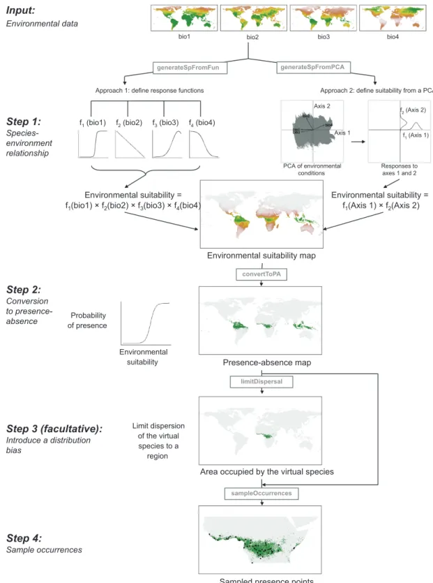
The package is structured around four major steps (Fig. 1): 1) generating virtual species’ environmental suitabil-ity from a spatial set of environmental conditions, with two different approaches (Meynard and Quinn 2007, Barbet-Massin et al. 2012); 2) converting the environmental suit-ability into presence–absence with a probabilistic approach (Meynard and Kaplan 2013); 3) introducing dispersal limi-tations in the realised virtual species distribution and 4) sampling occurrences with different biases in the sampling procedure. The package also includes various utility func-tions such as a function to visualise the species–environment relationships (Table 1). Hereafter, we detail the functioning of the package, step by step, and then we detail a working example of the package, showing how increasing ecological
realism in the generation of virtual species impacts the pre-dictive performance of SDMs. A comprehensive tutorial for the package is available online at < http://borisleroy.com/en/ virtualspecies >.
Package description
Requirements and input data
virtualspecies requires a standard installation of R and four extension packages, all of which can be installed from the Comprehensive R Archive Network: raster (Hijmans 2015), ade4 (Dray and Dufour 2007), dismo (Hijmans et al. 2014) and rworldmap (South 2011).
The package is designed to generate virtual species dis-tributions from spatial environmental datasets (Fig. 1). These environmental datasets are gridded spatial data in the ‘raster’ format of the R package raster. Specifically, vir-tualspecies uses RasterStack objects, i.e. piles of rasters with the same spatial extent and resolution, where each layer corresponds to an environmental variable. For example, the global climate dataset WorldClim (< www.worldclim. com >) can easily be imported into R to a RasterStack for-mat. Each layer of the input RasterStack corresponds to an environmental variable and must be named accordingly with a unique name. There is no limit to the number of layers of the input RasterStack, except for the capacities of the user’s computer.
Step 1 – generation of the virtual species’ environmental suitability
The basis of generating a virtual species distribution consists in simulating the environmental suitability of a species, i.e. simulating its response to different environmental gradi-ents, such as climatic variables. To simulate the environ-mental suitability, virtualspecies proposes two approaches (Fig. 1, step 1): 1) define a response function (e.g. linear, logistic, quadratic, gaussian) to each environmental vari-able, and combine these responses to define the environ-mental suitability (function generateSpFromFun); or 2) generate a principal component analysis (PCA) of all the environmental variables, define a response to each of the first two principal components (axes) and combine these responses to define the environmental suitability (function generateSpFromPCA).
1) Define responses to each environmental variable This approach was introduced by Hirzel et al. (2001) which generated a virtual species by defining response functions to different predictor variables (e.g. a linear increasing response to forest cover, or a Gaussian response to an elevation gradi-ent), and then combined the responses (using a weighted average) to obtain a habitat suitability value. It is the most frequently used approach to generate virtual species distri-butions (Elith et al. 2005, Meynard and Quinn 2007, Elith and Graham 2009, Bombi and D’Amen 2012, Meynard and Kaplan 2013). This approach is implemented in the func-tion generateSpFromFun. Several funcfunc-tions are embedded
Input:
Environmental data
f1 (bio1) f2 (bio2) f3 (bio3) f4 (bio4)
Environmental suitability = f1(bio1) × f2(bio2) × f3(bio3) × f4(bio4)
Environmental suitability = f1(Axis 1) × f2(Axis 2)
Environmental suitability map
Probability of presence
Environmental
suitability Presence-absence map
bio1 bio2 bio3 bio4
Approach 1: define response functions Approach 2: define suitability from a PCA
PCA of environmental conditions f1 (Axis 1) f2 (Axis 2) Axis 1 Axis 2 Responses to axes 1 and 2 Step 1: Species-environment relationship Step 2: Conversion to presence-absence Step 3 (facultative): Introduce a distribution bias Limit dispersion of the virtual species to a region
Area occupied by the virtual species
generateSpFromFun generateSpFromPCA convertToPA limitDispersal Step 4: Sample occurrences sampleOccurrences
Sampled presence points
Figure 1. Illustration of the package framework. The grey boxes on arrows indicate the names of the functions.
with virtualspecies, based on functions already used in the literature (Table 1). virtualspecies is also extremely flexible because any other function existing in R can be used as a response function to environmental conditions (such as the normal distribution: dnorm); response functions can also be entirely created by the user (see the virtualspecies tutorial, section 2.3. at http://borisleroy.com/en/virtualspecies ).
2) Define suitability from a PCA of environmental conditions
Defining response functions independently to each envi-ronmental variable (approach 1) can lead to virtual species with unrealistic environment conditions (e.g. a species with incompatible optima, such as an annual mean temperature of 35°C and a mean temperature of the warmest month of
a particular cell is turned into a presence or an absence. Therefore, a binomial experiment is run in each cell, with the probability of occurrence as the parameter. A cell with a probability of occurrence of 0.2 will be assigned a presence in 2 out of 10 cases under this probabilistic approach (for more details and examples see the online tutorial, sec-tion 4.1. at http://borisleroy.com/en/virtualspecies and Meynard and Kaplan 2013). This probabilistic conversion to presence–absence implies that repetitions of the conver-sion process will differ, each providing a valid realisation of the true species distribution map. However notice that this approach also provides the flexibility to simulate threshold as well as non-threshold responses (Meynard and Kaplan 2012, 2013). It is implemented in the function convertToPA.
The importance of species prevalence (i.e. the proportion of sites in which the species occurs), and particularly of the relationship between species prevalence and sample preva-lence (i.e. the proportion of samples in which the species has been found) has been demonstrated on SDMs (Meynard and Kaplan 2012). Hence, the function automatically cal-culates the species prevalence for the user. Alternatively, the user can also specify the desired species prevalence to the function, which will automatically determine an appropriate conversion curve.
Step 3 (facultative) – introduce a distribution bias One of the most disputed assumptions of SDMs is the assumption that species are at equilibrium with their environment (Guisan and Thuiller 2005), i.e. the assumption that they occupy their full range of suitable environmental conditions. This assumption is disputed 5°C). While such cases can easily be avoided when only a
few variables are considered, it becomes much more difficult when numerous variables are considered, especially if mul-tiple species are simulated. An alternative approach for such cases consists in generating a PCA of environmental condi-tions, and then defining responses to two axes of this PCA (Barve et al. 2011, Barbet-Massin et al. 2012). This approach ensures that the combination of environmental conditions is matched in the real world for the simulated species. It is implemented in the function generateSpFromPCA. This function is currently limited to the usage of normal response functions to the first two axes, but future versions will also implement any type of response function.
Step 2 – conversion of environmental suitability into presence–absence
The classical approach consists in defining a threshold to convert environmental suitability into a binary map of presence–absence (Hirzel et al. 2001, Bombi and D’Amen 2012). This approach, however, does not simulate the ran-dom processes acting on species occupancies and will always lead to threshold responses, despite the previous genera-tion of non-threshold environment–occurrence relagenera-tion- relation-ships (Meynard and Kaplan 2012, 2013). Such unrealistic virtual species can provide misleading results regarding the ability of modelling techniques to predict species distri-butions, particularly when non-threshold responses are of interest. An appropriate alternative consists in applying a probabilistic approach in which a logistic function is used first to convert environmental suitability into a probability of occurrence (Fig. 1, step 2). A subsequent random draw using the probability of occurrence determines whether
Table 1. Description of the functions included in the virtualspecies package. Many additional options and customisations are available for the functions, all of which are comprehensively documented in the help files of the package.
Core functions
generateSpFromFun Generates a virtual species suitability map by defining its response functions to environmental variables.
generateSpFromPCA Generates a virtual species suitability map by defining its response to a principal component analysis of environmental variables.
generateRandomSp Randomly generates a virtual species distribution, including the conversion to presence–absence. The random aspects can be customised.
convertToPA Converts the environmental suitability of a virtual species into presence–absence.
limitDistribution Introduces a bias in the distribution of a virtual species by limiting its distribution to a chosen area. sampleOccurrences Samples occurrence points of the virtual species, with or without biases.
Utility functions
formatFunctions Helps the user to format and illustrate the response functions as a correct input for generateSpFrom-Fun.
plotResponse Plots the relationship between the species and the environmental variables. Provides a plot appropriate for the method used to generate the virtual species.
removeCollinearity Analyses and (if chosen) removes the collinearity among the environmental variables.
synchroniseNA Ensures that cells containing NAs are the same among all the layers of a raster stack. Useful when building a stack of environmental variable coming from different sources, e.g. when combining climate with land use data.
Response functions currently embedded in the package
linearFun A linear function of the form ax b
logisticFun A logistic function of the form 1/(1 exp((x – b)/a)) quadraticFun A quadratic function of the form ax² bx c
custnorm A normal function parameterised by the mean, extreme values, and percentage of area under the curve between extremes.
and remove the collinearity among environmental variables (removeCollinearity). These functions are summarised in Table 1 and have many customisable parameters described in their associated help files.
Example of application: evolution of SDM
performance with increasing ecological
realism of virtual species
The generation of virtual species distributions is often aimed at testing modelling techniques and protocols, with the ulti-mate objective of transferring the results to real-world spe-cies. It is therefore important to attempt generating virtual species resembling real-world species. Hence, it is crucial to establish the degree of model performance overestima-tion when using virtual species with poor ecological realism. Here, we provide an example of this overestimation, using a very simple case study.
We built this example using previous works showing three frequent characteristics of real-world species that can be applied to virtual species. First, as explained in step 2, because of the random processes acting on species occupancies, real-world species are more likely to have a gradual response to the environment rather than a thresh-old response (Meynard and Kaplan 2012, 2013). Second, sampling procedures are scarcely perfectly randomised, and often there are strong disparities in sampling intensi-ties among geographical areas (see, e.g. the higher sampling intensity in Germany and the United Kingdom in spider distribution maps in Appendix S6 of Leroy et al. 2014), which impacts the performance of species distribution models (Phillips et al. 2009). Third, real-world species may not be at the equilibrium with their environment, as this has been shown for many invasive species (Václavík and Meentemeyer 2012).
Simulations
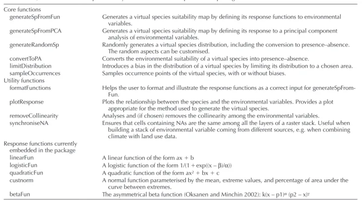
We generated a virtual species distribution on the basis of six bioclimatic variables ( www.worldclim.org/bioclim) : mean diurnal range (bio2), max temperature of warmest month (bio5), min temperature of coldest month (bio6), precipitation of wettest month (bio13), precipitation of driest month (bio14), precipitation seasonality (bio15). These variables were downloaded from WorldClim (www.worldclim.org) at a resolution of 0.17 decimal degrees, and the geographical area was restricted to the western Palearctic (longitude between –15 and 65; latitude between 30 and 75). On the basis of these environmental variables, we generated a virtual species’ environmental suit-ability with a PCA approach, using the generateSpFromPCA function. We manually defined the Gaussian response func-tions to axes 1 (mean 4, standard deviation 3) and 2 (mean 3, standard deviation 2). The resulting spe-cies–environment relationship was illustrated in Fig. 2 using the plotResponse function of the package.
From this single virtual species’ environmental suitability, we generated four cases of increasing complexity (see the R script in Supplementary material Appendix 1).
because species’ realised distributions are often assumed to be restricted to a subset of their potential distribu-tions, because of constraints to dispersal, competition, or stochastic extinction events for example. As a consequence, testing how well modelling techniques perform when the equilibrium assumption is violated is an important con-tribution of virtual species (Saupe et al. 2012). Virtual species generated with this package can be used to test such assumptions. The principle is to simulate a realised distribution for the virtual species which will be a sub-set of its potential distribution generated at step 2. This distribution bias can be achieved by different ways. Within the package, the function limitDistribution pro-vides several convenient ways to limit the distribution of the species (Fig. 1 step 3). This functions restricts species’ presences (defined at step 2) to a spatial area defined by the user, and thus precludes any presence in cells outside this area. For example, in Fig. 1 step 3, the virtual species’ distribution was restricted to conti-nental Africa only. To define the restricting area, differ-ent methods can be used in limitDistribution (i.e. using country, region or continent names, spatial polygons or extents).
Another possibility for users is to dynamically simu-late the dispersion of their virtual species by combining outputs from virtualspecies (environmental suitability generated at step 1) with other modelling plat-forms, such as the MIGCLIM R package (Engler et al. 2012) or RangeShifter (Bocedi et al. 2014). In Supplementary material Appendix 2, we detail an exam-ple where we simulate the dynamic dispersion of a vir-tual species in Great Britain by combining virvir-tualspecies with RangeShifter.
Step 4 – occurrence sampling
The last step consists in sampling observed occurrences for the virtual species with the function sampleOccurrences. This function can be used to sample different types of spe-cies occurrence (‘presence–absence’ or ‘presence only’), either randomly or with different biases similar to actual sampling biases (Fig. 1, step 4). For example, it is possible to assign a probability of detection to the virtual species, given the impact of imperfect detection on SDM perfor-mance (Lahoz-Monfort et al. 2014). This probability of detection can be weighted by environmental suitability, to simulate smaller populations in less suitable areas. An error probability can be defined, to simulate misiden-tifications (i.e. erroneous presence in cells where the species is absent). A sampling intensity bias can also be applied, to simulate over- or under-sampled areas (Phillips et al. 2009).
Utility functions
virtualspecies also includes various utility functions (Table 1), such as functions to visualise the relationship between the species and its environment (plotResponse), to randomly generate a virtual species (generateRandomSp),
only protocol, using 10 runs of 1000 randomly sampled pseudo-absences to calibrate generalised linear models with the default settings of biomod. We then projected the pre-dicted environmental suitability maps (averaged across the 10 pseudo-absence runs) of each case (Fig. 3) and calculated two performance metrics by comparing the true to the pre-dicted distributions for each case: the relative area under the receiver operating characteristic curve (ROC, Fielding and Bell 1997, ranging from 0.5 (no skill) to 1 (perfect score)) and the true skill statistic (TSS Allouche et al. 2006, rang-ing from 0 (no skill) to 1 (perfect score)). To compute the TSS metric, the predicted suitability maps were converted into presence–absence maps using a threshold maximising the TSS value.
Results
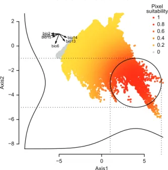
As expected, there was a progressive degradation of the ability of SDMs to correctly predict the environmental suitability (Fig. 3 B–D) as real-world aspects were included in the virtual species. Interestingly, the virtual distribution generated with a threshold conversion at step 2 was very well predicted above the threshold (i.e. above an environmental suitability of 0.7), but nothing could be predicted below the threshold (Fig. 3B). On the other hand, when a probabilistic conversion was used to generate the virtual species, SDMs were less performant to predict areas of high environmental suitability; but had the ability to detect the lower environmental suitability of the virtual species (Fig. 3C). When a sampling bias was intro-duced in Germany and the United Kingdom, the predicted suitability was even more biased. As expected, predicted suit-ability values showed higher values than true environmental suitability in areas with climate similar to these two countries, and lower predicted values than true environmental suitabil-ity elsewhere, such as in Spain and in eastern Europe (Fig. 3D). When the species was not at equilibrium with its envi-ronment, the predicted suitability was, unsurprisingly, dra-matically underestimated (Fig. 3E).
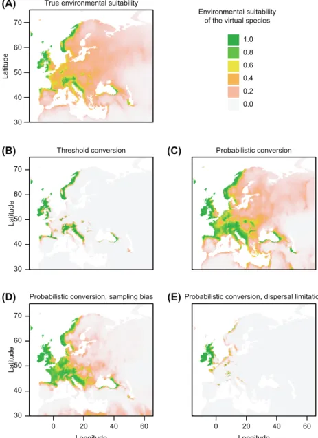
Regarding the performance of SDMs, when the species has a threshold response where it is always absent below a suitability threshold and always present above that threshold (case 1), SDMs generate near-perfect predictions according to both ROC and TSS (Fig. 4). However when the presence– absence corresponds to a probabilistic response (cases 2–4) there is a strong drop in predictive performance. The applied sampling bias (case 3) did further decrease the predictive per-formance, although to a lesser extent. Finally, SDMs applied on the species which was not at equilibrium with its environ-ment (case 4) yielded the most spectacular drop in predictive performance, compared to the other cases.
Implications
This simple example clearly illustrated how virtualspecies can be used to simulate distributions with increasing com-plexity and ask questions related to SDM performance. The case study show here confirmed the importance of using a probabilistic conversion into presence–absence (Meynard and Kaplan 2013). Results also extend the conclusions of Case 1: the environmental suitability was converted to
presence–absence using a threshold of 0.7 (above the thresh-old presence is attributed, below absence is attributed). 150 presence points were randomly sampled.
Case 2: the environmental suitability was converted to presence–absence with a logistic curve of parameters b 0.7 (inflexion point) and a –0.1 (steepness of the slope). 150 presence points were randomly sampled.
Case 3: same as case 2, except that a sampling bias was introduced, where Germany and the United Kingdom were 50 times more sampled than elsewhere. This sampling bias emulates a situation where these two countries have natural-ist societies who collected more data locally on the target species.
Case 4: same as case 2, except that the distribution of the species was subsequently limited to Great Britain and Ireland, using the function limitDistribution of the package. 150 presence points were randomly sampled.
Species distribution models
We built species distribution models for each case, using the biomod 2 modelling R package (Thuiller et al. 2009). We used the six raw climatic variables as predictors (i.e. not the axes of the PCA). We applied a classical
presence-−5 0 5 −8 −6 −4 −2 0 2
PCA of environmental conditions
Axis1 Axis2 bio2 bio5 bio6 bio13 bio14 bio15 Pixel suitability 1 0.8 0.6 0.4 0.2 0
Figure 2. Graphical representation of the simulation of a virtual species’ environmental suitability with a principal component anal-ysis (PCA) of six climate variables (acronyms detailed in main text). In the top left corner the projection of each input climate variables on the PCA is shown. Each point of the PCA corresponds to a pixel of the input raster of climate variables. The Gaussian responses of the species to each axis are illustrated next to their respective axis. An ellipse is drawn around the area where the pixel suitability is highest. Points are coloured according to their climate suitability values for the virtual species: red points correspond to pixels with the highest suitability, and yellow to grey points correspond to pix-els with the lowest suitability, as shown in the legend.
tion biases and sampling of occurrences. In this package we combined the best methodological advances from the litera-ture into this single framework. virtualspecies should there-fore help researchers in generating species with increased ecological realism, for example by designing complex spe-cies–environment relationships, avoiding the mistake of a threshold conversion into presence–absence (Meynard and Kaplan 2013), or introducing biases in the sampling of occurrence which are similar to real sampling biases (Phillips et al. 2009). Furthermore, virtualspecies can be coupled with other population dynamics platforms such as RangeShifter (Bocedi et al. 2014), which enables further complexity in the modelling of virtual species (Supplementary material Appendix 2).
Meynard and Kaplan (2012) to a situation where presence-only data are used, which was not tested in the previous study. Our package also allows adding further complexity to the simulations by incorporating dispersal limitations and sampling bias, two additional biases that, expectedly, also strongly impacted the predictive performance of SDMs.
Discussion
virtualspecies is the first package providing a full working framework to generate virtual species distributions, includ-ing the simulation of species–environment relationships, conversion into presence–absence, introduction of
distribu-30 40 50 60 70 Latitud e
True environmental suitability (A)
(B) (C)
(D) (E)
Environmental suitability of the virtual species
1.0 0.8 0.6 0.4 0.2 0.0 30 40 50 60 70 Latitud e
Threshold conversion Probabilistic conversion
30 40 50 60 70 Longitude Latitud e
Probabilistic conversion, sampling bias
0 20 40 60 0 20 40 60
Longitude
Probabilistic conversion, dispersal limitation
Figure 3. Maps of the (A) true and (B–E) predicted environmental suitability of the virtual species according to the different simulations: (B) conversion of environmental suitability to presence–absence with a threshold of 0.7; (C) conversion of environmental suitability to presence–absence with a logistic curve of parameters b 0.7 (inflexion point) and a –0.1 (steepness of the slope); (D) same simulation as in (C), but a sampling bias was introduced where Germany and the United Kingdom were 50 times more sampled than elsewhere; (E) same simulation as in (C), but the dispersal of the species was limited to Great Britain and Ireland.
0.8 0.9 1.0 0.4 0.6 0.8 1.0 ROC TS S Threshold
conversion Probabilistic conversion Probabilistic conversionSampling bias Probabilistic conversionDispersal bias
Type of virtual species
Performance metri
c
Figure 4. Boxplots of performance metrics of species distribution models for the different virtual species simulations. Each boxplot is based on the 10 pseudo-absence runs for the considered virtual species. ROC: area under the receiver operating characteristic curve; TSS: true skill statistic. The TSS was evaluated on maps of pres-ence–absence predicted using a conversion threshold maximising the TSS value.
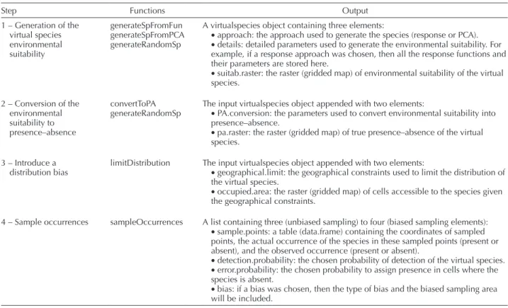
Table 2. Steps of the framework, associated functions of the virtualspecies R package, and output objects.
Step Functions Output
1 – Generation of the virtual species environmental suitability generateSpFromFun generateSpFromPCA generateRandomSp
A virtualspecies object containing three elements:
• approach: the approach used to generate the species (response or PCA). • details: detailed parameters used to generate the environmental suitability. For example, if a response approach was chosen, then all the response functions and their parameters are stored here.
• suitab.raster: the raster (gridded map) of environmental suitability of the virtual species. 2 – Conversion of the environmental suitability to presence–absence convertToPA
generateRandomSp The input virtualspecies object appended with two elements:• PA.conversion: the parameters used to convert environmental suitability into presence–absence.
• pa.raster: the raster (gridded map) of true presence–absence of the virtual species.
3 – Introduce a
distribution bias limitDistribution The input virtualspecies object appended with two elements:• geographical.limit: the geographical constraints used to limit the distribution of the virtual species.
• occupied.area: the raster (gridded map) of cells accessible to the species given the geographical constraints.
4 – Sample occurrences sampleOccurrences A list containing three (unbiased sampling) to four (biased sampling elements): • sample.points: a table (data.frame) containing the coordinates of sampled points, the actual occurrence of the species in these sampled points (present or absent), and the observed occurrence (present or absent).
• detection.probability: the chosen probability of detection of the virtual species. • error.probability: the chosen probability to assign presence in cells where the species is absent.
• bias: if a bias was chosen, then the type of bias and the biased sampling area will be included.
In this paper we provided a very simple example showing how the performance of SDMs can be altered when applying different real-world aspects on virtual species. The four cases of our example were generated with only a few lines of code (Supplementary material Appendix 1), which clearly
high-lights the simplicity of generating multiple different cases with the virtualspecies R package. The combination of its simplicity of use and possibilities of customisation will allow ecologists to easily generate multiple virtual species distribu-tions with a fine control over the different simulation param-eters. For example, the function generateSpFromFun can use any user-defined response function. As a consequence, researchers willing to test a very particular response func-tion, specific to model organisms, will be able to use virtu-alspecies, such as the different thermal performance curves described in Angilletta (2006). This will allow researchers to test new hypotheses, for example regarding the distribution of actual species or the robustness of modelling techniques to unusual species–environment relationships. In addition, the possibility of controlling every simulation parameter is valuable when generating virtual species distributions to test the robustness of modelling techniques and protocols to par-ticular aspects or biases (Miller 2014).
Another major contribution of virtualspecies is an enhancement of transparency, replicability and compara-bility of studies involving virtual species. Indeed, the gen-erated virtual species can be stored on the hard disk drive and provided in online supplementary materials of articles. Likewise, all the parameters used to generate virtual species are stored in the package outputs (Table 2), and can be pro-vided in articles. These parameters can then be used as inputs to generate the same virtual species (see e.g. the R script in Supplementary material Appendix 1 to reproduce the exam-ple of this article), including the random aspects if the users use the R function set.seed before their simulations.
Given the importance of SDMs in ecology, biogeogra-phy and biological conservation, and the fact that many methodological aspects of SDMs still need improvement,
we expect that virtual species will have a major positive impact in these fields. We also expect virtual species to be useful in other fields. For example, virtual species can pro-vide insights to test issues in biogeography, such as niche conservatism, but also to test hypotheses at micro-scales, such as the impact of climate change on the distribution of insects on plant surfaces.
To cite virtualspecies or acknowledge its use, cite this Software note as follows, substituting the version of the application that you used for ‘version 0’:
Leroy, B., Meynard, C. N., Bellard, C. and Courchamp, F. 2015. virtualspecies, an R package to generate virtual species distribu-tions. – Ecography 39: 599–607 (ver. 0).
Acknowledgements – BL, CB and FC were funded under the FFII
ERA-NET BiodivERsA project. We thank Wilfried Thuiller for fruitful discussions and wise advices and Régis Gallon for beta-testing the package. This is VIMS contribution no. 3466.
References
Allouche, O. et al. 2006. Assessing the accuracy of species distribu-tion models: prevalence, kappa and the true skill statistic (TSS). – J. Appl. Ecol. 43: 1223–1232.
Angilletta, M. J. 2006. Estimating and comparing thermal per-formance curves. – J. Therm. Biol. 31: 541–545.
Barbet-Massin, M. et al. 2012. Selecting pseudo-absences for spe-cies distribution models: how, where and how many? – Meth-ods Ecol. Evol. 3: 327–338.
Barve, N. et al. 2011. The crucial role of the accessible area in ecological niche modeling and species distribution modeling. – Ecol. Model. 222: 1810–1819.
Bellard, C. et al. 2013. Will climate change promote future inva-sions? – Global Change Biol. 19: 3740–3748.
Bocedi, G. et al. 2014. RangeShifter: a platform for modelling spatial eco-evolutionary dynamics and species’ responses to environmental changes. – Methods Ecol. Evol. 5: 388–396. Bombi, P. and D’Amen, M. 2012. Scaling down distribution maps
from atlas data: a test of different approaches with virtual spe-cies. – J. Biogeogr. 39: 640–651.
Dray, S. and Dufour, A.B. 2007. The ade4 package: implementing the duality diagram for ecologists. – J. Stat. Softw. 22: 1–20. Duan, R.-Y. et al. 2015. SDMvspecies: a software for creating
vir-tual species for species distribution modelling. – Ecography 38: 111–220.
Elith, J. and Graham, C. H. 2009. Do they? How do they? WHY do they differ? On finding reasons for differing performances of species distribution models. – Ecography 32: 66–77. Elith, J. et al. 2005. The evaluation strip: a new and robust method
for plotting predicted responses from species distribution mod-els. – Ecol. Model. 186: 280–289.
Elith, J. et al. 2006. Novel methods improve prediction of species’ distributions from occurrence data. – Ecography 29: 129–151. Elith, J. et al. 2010. The art of modelling range-shifting species.
– Methods Ecol. Evol. 1: 330–342.
Engler, R. et al. 2012. The MIGCLIM R package – seamless integration of dispersal constraints into projections of species distribution models. – Ecography 35: 872–878.
Fielding, A. H. and Bell, J. F. 1997. A review of methods for the assessment of prediction errors in conservation presence/ absence models. – Environ. Conserv. 24: 38–49.
Guisan, A. and Thuiller, W. 2005. Predicting species distribution: offering more than simple habitat models. – Ecol. Lett. 8: 993–1009.
Hijmans, R. J. 2015. raster: geographic data analysis and modeling. – R package ver. 2.3-24, < http://CRAN.R-project. org/package = raster >.
Hijmans, R. J. et al. 2014. dismo: species distribution modeling. – R package ver. 0.3.1, < http://CRAN.R-project.org/ package = dismo >.
Hirzel, A. H. et al. 2001. Assessing habitat-suitability models with a virtual species. – Ecol. Model. 145: 111–121.
Kong, X.-Q. et al. 2014. Create virtual species with sdmvspecies. – R package ver. 0.3.1, < http://cran.r-project.org/package = sdmvspecies >.
Lahoz-Monfort, J. J. et al. 2014. Imperfect detection impacts the performance of species distribution models. – Global Ecol. Biogeogr. 23: 504–515.
Leroy, B. et al. 2013. First assessment of effects of global change on threatened spiders: potential impacts on Dolomedes
plantarius (Clerck) and its conservation plans. – Biol. Conserv.
161: 155–163.
Leroy, B. et al. 2014. Forecasted climate and land use changes, and protected areas: the contrasting case of spiders. – Divers. Distrib. 20: 686–697.
Meynard, C. N. and Quinn, J. F. 2007. Predicting species distributions: a critical comparison of the most common statistical models using artificial species. – J. Biogeogr. 34: 1455–1469.
Meynard, C. N. and Kaplan, D. M. 2012. The effect of a gradual response to the environment on species distribution modeling performance. – Ecography 35: 499–509.
Meynard, C. N. and Kaplan, D. M. 2013. Using virtual species to study species distributions and model performance. – J. Bio-geogr. 40: 1–8.
Miller, J. A. 2014. Virtual species distribution models: using simu-lated data to evaluate aspects of model performance. – Prog. Phys. Geogr. 38: 117–128.
Oksanen, J. and Minchin, P. 2002. Continuum theory revisited: what shape are species responses along ecological gradients? – Ecol. Model. 157: 119–129.
Phillips, S. J. et al. 2009. Sample selection bias and presence-only distribution models: implications for background and pseudo-absence data. – Ecol. Appl. 19: 181–197.
Saupe, E. E. et al. 2012. Variation in niche and distribution model performance: the need for a priori assessment of key causal factors. – Ecol. Model. 237–238: 11–22.
Schumaker, N. H. 2015. HexSim version 3.0. – U.S. Environmen-tal Protection Agency, EnvironmenEnvironmen-tal Research Laboratory, Corvallis, USA, www.hexsim.net .
South, A. 2011. rworldmap: a new R package for mapping global data. – R J. 3: 35–43.
Strubbe, D. et al. 2013. Niche conservatism in non-native birds in Europe: niche unfilling rather than niche expansion. – Global Ecol. Biogeogr. 22: 962–970.
Thibaud, E. et al. 2014. Measuring the relative effect of factors affecting species distribution model predictions. – Methods Ecol. Evol. 5: 947–955.
Thuiller, W. et al. 2009. BIOMOD – a platform for ensemble fore-casting of species distributions. – Ecography 32: 369–373. Václavík, T. and Meentemeyer, R. K. 2012. Equilibrium or not?
Modelling potential distribution of invasive species in different stages of invasion. – Divers. Distrib. 18: 73–83.
Varela, S. et al. 2014. Environmental filters reduce the effects of sampling bias and improve predictions of ecological niche models. – Ecography 37: 1084–1091.
Supplementary material (Appendix ECOG-01388 at < www.ecography.org/appendix/ecog-01388 >). Appendix 1–2.