The application of optimal control theory to dynamic routing in data communication networks.

THE APPLICATION OF OPTIMAL CONTROL THEORY TO DYNAMIC ROUTING IN DATA COMMUNICATION NETWORKS

by

FRANKLIN HOWARD MOSS B.S.E., Princeton University

1971

S.M., Massachusetts Institute of Technology 1972

SUBMITTED IN PARTIAL FULFILLMENT OF THE REQUIREMENTS FOR THE DEGREE OF DOCTOR OF PHILOSOPHY

at the

MASSACHUSETTS INSTITUTE OF TECHNOLOGY February 1977

7

Signature of Author. --... - .-.-.-..

.-/ Department of Aeronautics and Astronautics -q -2 November 24, 1976 Certified by... Certified (7 Thesis Supervisor

by...-.-.-....-..----..

Departmental Graduate Committee

FRANKLIN HOWARD MOSS

Submitted to the Department of Aeronautics and Astronautics in partial fulfillment of the requirements for the degree of Doctor of Philosophy.

ABSTRACT

The flow of messages in a message-switched data communication net-work is modeled in a continuous dynamical state space. The state vari-ables represent message storage at the nodes and the control varivari-ables represent message flow rates along the links. A deterministic linear cost functional is defined which is the weighted total message delay in the network when we stipulate that all the message backlogs are emptied at the final time and the inputs are known. The desired mini-mization of the cost functional results in a linear optimal control problem with linear state and control variable inequality constraints.

The remainder of the thesis is devoted to finding the feedback solution to the optimal control problem when all the inputs are con-stant in time. First, the necessary conditions of optimality are

derived and shown to be sufficient. The pointwise minimization in time is a linear program and the optimal control is seen to be of the bang-bang variety. Utilizing the necessary conditions it is shown that the

feedback regions of interest are convex polyhedral cones in the state space. A method is then described for constructing these regions from a comprehensive set of optimal trajectories constructed backward in time from the final time. Techniques in linear programming are

em-ployed freely throughout the development, particularly the geometrical

interpretation of linear programs and parametric linear programming. There are several properties of the method which complicate its formulation as a compact algorithm for general network problems.

How-ever, in the case of problems involving networks with single

destina-tions and all unity weightings in the cost functional it is shown that

these properties do not apply. A computer implementable algorithm is then detailed for the construction of the feedback solution.

-2-

-2a-Thesis Supervisor: Adrian Segall

Title: Assistant Professor Electrical Engineering Thesis Supervisor: Wallace E. Vander Velde

Title: Professor of Aeronautics and Astronautics Thesis Supervisor: Alan S. Willsky

toral Committee for invaluable counsel and unfailing personal support. Professor Adrian Segall stimulated my interest in data communication networks, suggested the topic of this thesis, and generously contri-buted of his time as colleague and friend during this research. From him I have learned that perserverance is the most important part of

research. Professor Wallace E. Vander Velde, chairman of the committee, has served as mentor and teacher throughout my doctoral program. His wise advice, with regard to this thesis and other matters, is greatly

appreciated. My association with Professor Alan S. Willsky, both during thesis research and previously, has been most rewarding. His intellectual and personal energy, combined with a fine sense of humor, provide an atmosphere which I find both stimulating and enjoyable.

My research experience at the Electronic Systems Laboratory has been a very pleasant and productive one. I offer my heartfelt thanks

to those faculty members, staff members and fellow students who have helped make it so. In particular: to Professor John M. Wozencraft, for graciously providing the administrative support which made this research possible; to Professor Sanjoy K. Mitter, for serving as a thesis reader and sharing of his expertise in optimal control theory; to Professor

-3-

-4-Robert G. Gallager, for serving as a thesis reader and providing valuable comments on the message routing problem; to Dr. Stanley B. Gershwin, for many interesting discussions and suggestions; to Ms.

Susanna M. Natti, for unselfishly forsaking her art career to apply her creative talents to the expert preparation of the manuscript; to Ms. Myra Sbarounis for efficiently and cheerfully administering to

everyday affairs; and finally, to my officemates Mr. Martin Bello and Mr. James R. Yee (graduate students always come last) for maintaining

a suitably chaotic atmosphere.

The support of my entire family during my graduate career, and during my education as a whole, has been my greatest incentive. I cannot adequately thank here my parents, Samuel and Rose, my brother Billy and sister Ivy for a lifetime of love and encouragement. It is certainly hopeless to describe in a few words what has been given me by Janie during four years of marriage - unwavering support, sacrifice, and love to be sure - but more than that, what it takes to make life

sweet. I thank her every day. We are both ever thankful for our son Ilan, who always makes us smile. In appreciation, I dedicate this thesis to my family.

ABSTRACT

ACKNOWLEDGEMENTS TABLE OF CONTENTS

Chapter 1 INTRODUCTION

1.1 Introduction to Data Communication Networks 1.2 Discussion of the Message Routing Problem 1.3 Thesis Overview

1.3.1 Objective of Thesis

1.3.2 Approach

1.3.3 Preview of Results 1.4 Synopsis of Thesis

Chapter 2 NEW DATA COMMUNICATION NETWORK MODEL AND OPTIMAL CONTROL PROBLEM FOR DYNAMIC ROUTING 2.1 Introduction

2.2 Basic Elements of the State Space Model 2.2.1 Topological Representation

2.2.2 Message Flow and Storage Representation 2.3 Dynamic Equations and Constraints

2.4 Performance Index and Optimal Control Problem Statement -5-2 3 5 9 9 12 17 17 18 20 23 26 26 28 28 29 33 35

-6-Page 2.5 Discussion of the Optimal Control Problem

2.6 Previous Work on Optimal Control Problems with State Variable Inequality Constraints

2.7 Open Loop Solutions

2.7.1 Linear Programming Through Discretization 2.7.2 Penalty Function Method

Chapter 3 FEEDBACK SOLUTION TO THE OPTIMAL CONTROL PROBLEM WITH CONSTANT INPUTS

3.1 Introduction

3.2 Feedback Solution Fundamentals

3.2.1 Necessary and Sufficient Conditions 3.2.2 Controllability to Zero for Constant

Inputs

3.2.3 Geometrical Characterization of the Feedback Space for Constant Inputs

3.3 Backward Construction of the Feedback Space for

Constant Inputs

3.3.1 Introductory Examples of Backward Boundary

Sequence Technique

3.3.2 Technique for the Backward Construction of the Feedback Space

3.3.2.1 Preliminaries

3.3.2.2 Description of the Algorithm 3.3.2.3 Discussion of the Algorithm 3.3.3 Basic Procedures of the Algorithm

39 41 45 45 47 50 50 52 52 67 72 91 91 113 113 115 135 142

3.3.3.1 Solution of Constrained Optimization Problem

3.3.3.2 Determination of Leave-the-Boundary Costates, Subregions

and Global Optimality 3.3.3.3 Construction of Non-Break

Feedback Control Regions 3.3.3.4 Construction of Break

Feedback Control Regions 3.3.4 Discussion of Fundamental Properties of

the Algorithm 3.3.4.1 Non-Global Optimality of Certain Sequences 3.3.4.2 Non-Uniqueness of Leave-the-Boundary Costates 3.3.4.3 Subregions

3.3.4.4 Return of States to Boundary Backward in Time

3.4 Summary

r 4 FEEDBACK ROUTING WITH CONSTANT INPUTS WEIGHTINGS

4.1 Introduction 4.2 Preliminaries

4.3 Special Properties of the Algorithm

4.4 Computational Algorithm

4.5 Extension to General Network Problems

Chapter 5 5.1 AND UNITY CONCLUSION Discussion 142 147 168 175 180 181 186 190 196 202 204 204 206 216 267 278 284 284 Chapte

-8-5.2 Summary of Results and Related Observations 5.2.1 Results

5.2.2 Related Observations 5.3 Contributions

5.4 Suggestions for Further Work Appendix A

Appendix B

REFERENCES BIOGRAPHY

FINDING ALL EXTREME POINT SOLUTIONS TO THE CONSTRAINED OPTIMIZATION PROBLEM

EXAMPLE OF NON-BREAK AND BREAK FEEDBACK CONTROL REGIONS Page 288 288 289 292 293 296 299 302 305

1.1 Introduction to Data Communication Networks

A data communication network is a facility which interconnects a number of data devices (such as computers and terminals) by communica-tion channels for the purpose of transmission of data between them. Each device can use the network to access some or all of the resources available throughout the network. These resources consist primarily of computational power (CPU time), memory capacity, data bases and specialized hardware and software. With the rapidly expanding role being played by data processing in today's society (from calculating

interplanetary trajectories to issuing electric bills) it is clear that the sharing of computer resources is a desirability. In fact, the distinguished futurist Herman Kahn of the Hudson Institute has forecast that the "marriage of the telephone and the computer" will be one of the most socially significant technological achievements of the next two hundred years.

Research in areas related to data communication networks began in the early 1960's and has blossomed into a sizable effort in the 1970's. The ARPANET (Advanced Research Projects Agency NETwork) was implemented in 1970 as an experimental network linking a variety of university,

-9-

-10-industrial and government research centers in the United States. Cur-rently, the network connects about one hundred computers throughout the continental United States, Hawaii and Europe. The network has enjoyed considerable success and as a result several other major net-works are presently being planned.

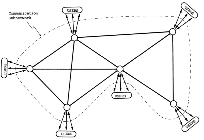
Following Kleinrock [1976), we now describe the basic components of a data communication network and their functions. Fundamentally, what is known as the communication subnetwork consists of a collection

of nodes which exchange data with each other through a set of links. Each node essentially consists of a minicomputer which may have data

storage capability and which serves the function of directing data which passes through the node. The links are data transmission chan-nels of a given data rate capacity. The data devices which utilize the communication subnetwork, known as users, insert data into and receive data from the subnetwork through the nodes. See Figure 1.1. A more detailed description of the network in the context of the

analysis of this thesis is presented in Chapter 2.

The data travelling along the links of the network is organized into messages, which are groups of bits which convey some information. One categorization of networks differentiates those which have message storage at the nodes from those which do not. Those with storage are known as store-and-forward networks. Another classification is made according to the manner in which the messages are sent through the network. In a circuit-switching network, one or more connected chains

Figure 1.1 Data Communication Network

I Hj

-12-of links is set up from the node -12-of origin to the destination node -12-of of the message, and certain proportions of data traffic between the

origin and destination are then transmitted along these chains. The other category includes both message switching and packet switching

networks. In message-switching, only one link at a time is used for the transmission of a given message. Starting at the source node the message is stored in the node until its time comes to be transmitted on an outgoing link to a neighboring node. Having arrived at that node it is once again stored until being transmitted to the next node. The message continues to traverse links and wait at nodes until it finally reaches its destination. Packet-switching is fundamentally the same

as message switching, except that a message is decomposed into smaller pieces of maximum length called packets. These packets are properly

identified and work their way through the network in the fashion of message switching. Once all packets belonging to a given message arrive at the destination node, the message is reassembled and delivered to the user. In this thesis we shall be concerned with store-and-forward networks which employ message(packet)-switching.

1.2 Discussion of the Message Routing Problem

There is a myriad of challenging problems which must be confronted in the design and operation of data communication networks. Just to name a few, there are the problems of topological design (cost effective

network from their nodes of origin to their nodes of destination. The latter problem is one of the fundamental issues involved in the opera-tion of networks and as such has received considerable attenopera-tion in the data-communication network literature. It is clear that the efficiency with which messages are sent to their destinations determines to a great extent the desirability of networking data devices. The subjective term "efficient" may be interpreted mathematically in many ways, depending on the specific goals of the network for which the routing procedure is being designed. For example, one may wish to minimize total message delay, maximize message throughput, cost. etc. In general, this issue

is referred to as the routing problem. We shall be concerned with the minimum delay message routing problem in this thesis.

Routing procedures can be classified according to how dynamic they are. At one end of the scale we have purely static strategies in which fractions of the message traffic at a given node with a given destination are directed on each of the outgoing links, where the frac-tions do not change with time. On the other end of the scale we have completely dynamic strategies, which allow for continual changing of the routes as a function of time, and also as a function of message congestion and traffic requirements in the network. Static procedures are easier to implement than dynamic ones, but lack the important

ability to cope with changing congestion and traffic requirements in the network possessed by dynamic strategies.

-14-Although a large variety of routing procedures have been developed and implemented in existing networks (such as ARPANET) the lack of a basic model and theory able to accommodate various important aspects of the routing problem has made it necessary to base the procedures almost

solely on intuition and heuristics. Of concern here is the fact that previous techniques have been addressed primarily to static routing

strategies, which lack the previously discussed advantages of dynamic strategies. The best known approach to static message routing in store-and-forward data communications networks is due to

Kleinrock

[1964]. This approach is based upon queueing theory and we describe the principal elements here briefly for comparison with the dynamic method which we shall discuss subsequently:

(a) The messages arrive from users to the network according to independent constant rate Poisson processes and their lengths are assumed to be independent exponentially distributed and independent of

their arrival times.

(b) At subsequent nodes along the paths of the messages, the

lengths of the messages and their interarrival times become dependent, a fact which makes the analysis extremely difficult. To cope with this problem, the famous independence assumption is introduced, requiring the messages to "lose their identities" at each node and to be assigned new independent lengths.

(c) once a message arrives at a node, it is first assigned to one of the outgoing links and waits in queue at that link until it is

transmitted.

(d) Based on queueing analysis, the average delay in steady state experienced by messages in each link is calculated explicitly in terms of the various arrival rates, average message length and the capacity of the link.

(e) A routing procedure is then found to minimize the average delay over the entire network. See Cantor and Gerla [1974].

The routing procedure thus obtained is static, namely constant in time and a function only of the various average parameters of the sys-tem. In the parlance of control theory, which is the language which we shall be using for much of this thesis, such a strategy is referred to as open-loop.

Since Kleinrock's model was proposed in 1962, researchers in the area have repeatedly expressed the desire to find approaches to other aspects of the routing problem. In particular, the goal is to find an approach

(i) in which the independence assumption is not required,

(ii) that will be able to handle transients and dynamical situa-tions and not only steady state, and

(iii) that can lead to optimal closed-loop control strategies, namely strategies that change according to the congestion

in the network.

Requirement (i) is desirable since the independence assumption may be quite inappropriate in various situations. Furthermore, it is not

-16-easy to assess the validity of this assumption for a given network. The desirability of requirement (ii) has been discussed previously. Finally, perhaps the most important requirement is (iii), for it is a fundamental fact of optimal control theory that closed-loop strategies are much less sensitive than open-loop ones to perturbations.in the parameters of the system. Hence, occurrences such as link and node

failures or unexpected bursts of user input to the network are accom-modated much better by closed-loop strategies.

It is pointed out in Segall [1976] that the traditional queueing theory approach can in principle be adapted to closed loop strategies, but that the number of states required would be immense. This approach looks at each message or packet as an entity, and therefore the state of the network is described by the number and destination of messages

(packets) in each of the buffers. Therefore, in a network with N nodes, S outgoing links per node in the average and buffers of maximum capacity of M messages (packets), the number of states is approximately ( NM)N-1 which is an extremely large number even for the smallest of networks.

Segall [1976] has introduced a model for message routing which is capable of achieving requirements (i)-(iii) above. His approach is to model the flow of messages in a message (packet)-switched store-and-forward data communication network in a continuous dynamical state space setting. The continuous nature of the state is justified by recognizing that any individual message contributes very little to the overall behavior of the network, so that it is not necessary to look

individually at each of the messages and their lengths. In this vein, it makes more sense to regard the network in the more macroscopic fashion of Segall's model.

Having established the model, Segall expresses the minimum delay dynamic routing problem as a linear optimal control problem with linear state and control variable inequality constraints for which a feedback

solution is sought. Should such a solution to this problem be obtained, the resulting strategy would be dynamic and closed-loop. The model and associated optimal control problem are discussed briefly in the next

section and are presented in detail in Chapter 2.

1.3 Thesis Overview

1.3.1 Objective of Thesis

The goal of this research is to obtain feedback solutions to the linear optimal control problem with linear state and control variable inequality constraints suggested by Segall for the message routing problem. Undoubtedly, the principal difficulty presented by this prob-lem is the presence of state variable inequality constraints. This contention is supported by the observation that very few feedback

solu-tions have been found for optimal control problems with this type of constraint. We clearly shall have to exploit the special properties

of our problem (such as linearity and the structure of the dynamics and constraints) to develop new theory and techniques capable of producing feedback solutions.

-18-1.3.2 Approach

We begin our discussion of approach by briefly describing Segall's state space model. In the model the state variables represent the quan-tity of messages stored at the nodes, distinguished according to node of current residence and node of ultimate destination. In reality, the measure of message storage at the nodes is a discrete variable (such as number of messages, packets, bits, etc.). However, in the spirit of viewing the network from a macroscopic point of view, we assume that the units of data traffic are such that after appropriate normalization

the states may be approximated closely by continuous variables. The control variables represent the flow rate of traffic in the links, where each control represents that portion of a given link's rate capacity devoted to transmitting messages of a given destination. Finally, the inputs are the flow rates of messages entering the network from the users. In this thesis, we consider the inputs to be deterministic functions of time. The dynamical equation which represents the flow of messages in the network is

x(t) = B u(t) + a(t) _(1.1)

where x(t), u(t) and a(t) are the vectors of state variables, control variables and inputs respectively. In the static flow literature the matrix B is known as the "incidence matrix", and it is composed solely of +1's, -l's and O's which capture the node-link configuration of the network. We also have several essential constraints. The state

varia-ble inequality constraints are x(t) > 0 for all t, since the message

storage must always be non-negative. The control variable inequality

constraints are u(t) C U for all t, where

U

We now associate with the dynamical state space model the linear cost functional

=

tfa

0

where x(t0

)

a

for now that when a is all l's, then J is exactly the total delay ex-perienced by all of the messages traveling through the network on

[t0, tf ]. By adjusting the values of the elements of a, J may be made

to represent a desired form of weighted total delay. The optimal control problem which represents the dynamic feedback message routing problem is:

Find the control u(t) as a function of time and state, u(t) E u(t, x), that will bring the state from x(t 0) = x

(given) to x(t f) = 0 while minimizing J subject to the dynam-ics and state and control variable inequality constraints.

-20-Our approach to solving the above problem shall now be described briefly. We begin by deriving the necessary conditions of optimality associated with the optimal control problem and prove that they are also sufficient. Realizing that there is extremely little hope of ob-taining at this time a feedback solution for the general deterministic input problem, we restrict the inputs to be constant in time. The necessary conditions indicate that with this assumption the optimal

feedback control is regionwise constant over the state space. We then develop a procedure which utilizes the necessary conditions to construct all of these regions and identify their associated optimal controls. Although the procedure is not readily implementable on the computer for problems involving general multi-destination networks, we are able to

utilize special structural properties of the problem to devise a com-puter algorithm for problems involving single destination networks with

all unity weightings in the cost functional.

1.3.3 Preview of Results

In this section we elaborate on the discussion of approach of the previous section and simultaneously describe the highlights of the results which are obtained.

According to the necessary conditions which are derived for the problem, any optimal control must satisfy

u*(t) = ARG MIN (X (t)B u(t)) (1.3)

u(t) CU

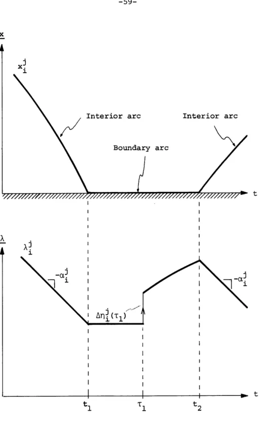
cor-responding to the state x(t) and is given by a linear differential equation with free terminal conditions. Of particular interest is the fact that a costate may exhibit discontinuities at times when its associated state is traveling on a boundary arc x = 0. We are also

able to prove the significant result that the necessary conditions of optimality are also sufficient.

For given values of the costate vector, the pointwise minimization is a linear program. Owing to fundamental properties of linear

pro-gramming we are able to deduce the following: (i) the optimal control

always lies at boundary points of

U,

(iii) the minimization need not be performed at every time, but may be solved parametrically in time to find the optimal bang-bang controls and switch times.

Note that all of the above results apply for general deterministic inputs. Henceforth we restrict ourselves to the special case in which the inputs are constant in time. In this case, the bang-bang nature of the optimal control implies that the slope of the optimal state trajec-tory is piecewise constant in time. We are now able to state and prove sufficiency conditions under which any initial state x(t0 ) =

O

controllable to x(t ) = 0 for a given network with given set of constant inputs.

Using the necessary conditions, we are able to show that the optimal control is regionwise constant and that the regions are convex polyhedral cones in the state space. A procedure is then developed

-22-which employs the spirit of dynamic programming to construct these cones and their associated optimal controls by a sequence of backward optimal trajectories propagating from the final time t f When a sufficiently

large variety of these trajectories is utilized to construct regions, the union of these regions fills up the state space with optimal

con-trols, thus constituting the feedback solution.

In order to solve for the backward optimal trajectory, we must propagate the costates backward in time according to their differential

equation and solve the minimization problem (1.3) for all solutions. However, there is a question regarding the appropriate values of the

costates which realize a particular backward optimal trajectory through (1.1) and (1.3). The resolution to this problem is geometrical in nature in that it considers the Hamiltonian function associated with the necessary conditions to be a hyperplane which is continuously rota-ting about the constrained region of message flow while remaining

tangent to it. As the costates are the coefficients of the hyperplane, their appropriate values are determined by orienting the hyperplane in

a prescribed fashion with respect to the constraint region. This argu-ment freely employs geometrical concepts in linear programming.

We are unable to devise a computer algorithm to implement the above procedure for general multi-destination network problems due to several complicating properties. However, we are able to show that for problems involving single destination networks with all unity weightings in the cost functional these complicating properties do not apply. A

computational implementation of the procedure is then readily formu-lated and a computer example is performed. It turns out that one of the computational tasks of the algorithm is extremely inefficient. This task is involved with the problem of finding all of the non-unique extremal solutions to a linear program. As a consequence, the computa-tional feasibility of the algorithm is contingent upon the development of a more efficient technique for solving this problem.

In evaluating the ultimate desirability of the feedback

approach, we must take into account the fact that considerable computer storage may be required to implement the feedback solution on line. This results from the necessity of storing all of the linear inequali-ties which specify the convex polyhedral cones in the state space, and there may be many such cones. A tradeoff is therefore in order between the storage involved to implement closed-loop solutions and the computation involved in the implementation of open loop solutions.

1.4 Synopsis of Thesis

The purpose of this section is to provide a brief summary of the remaining chapters.

Chapter 2

The state space model and optimal control problem of Segall are described in detail. A brief discussion is devoted to two possible open-loop solutions: The first employs linear programming through

-24-technique. Note that although they are open-loop, these techniques are dynamic.

Chapter 3

In this chapter we present the procedure for the synthesis of a feedback solution to the optimal control problem with constant inputs. We begin by deriving the necessary conditions of optimality and prove that they are sufficient. Based upon these conditions we characterize the feedback regions of interest as convex polyhedral cones. After providing a few motivating examples, we present the algorithm for the

backward construction of the feedback control. Finally, we isolate

and describe in detail those properties of the algorithm which

compli-cate its computational implementation.

Chapter 4

The geometrical linear programming interpretation is utilized to construct proofs that the complicating properties of the algorithm of Chapter 3 do not apply for problems involving single destination net-works with all unity weightings in the cost functional. This fortuitous situation enables us to construct an algorithm which is implementable on the computer. An example is run for a five node network. We then present thoughts on how the techniques of this chapter may be applied to general multi-destination network problems with non-unity weightings in the cost functional.

Chapter 5

In this chapter we comment on various aspects of the approach in general and of the feedback control algorithm in particular. Some insight is provided into related topics not specifically discussed in preceding chapters. We then summarize our results, present the spe-cific contributions and make suggestions for further work in this area.

Chapter 2

NEW DATA COMMUNICATION NETWORK MODEL AND OPTIMAL CONTROL PROBLEM FOR DYNAMIC ROUTING

2.1 Introduction

In this chapter, the flow and storage of messages in a message-(packet)-switched store-and-forward data communication network are ex-pressed in a dynamical state space setting. This model for routing was

introduced by Segall [1976). The principal elements of the model - state variables, control variables, and inputs - are defined to represent

mathematically the fundamentals of network operation: storage, traffic flow and message input respectively. Emerging from this characteriza-tion is an ordinary linear vector differential equacharacteriza-tion which dynami-cally describes the storage state of the network at every time. State variable positivity constraints and control variable capacity con-straints, both linear, are imposed as an essential part of the model. Presently, we assume that the inputs are deterministic functions of time, representing a scheduled rate of demand.

Arising naturally out of the model as defined is a linear inte-gral cost functional which is equal to the total delay experienced by all of the messages travelling in the network. Owing to the generality of our expression, we are also able to formulate a linear cost

function-al which corresponds to a measure of weighted message delay in the

-26-work. Combining the minimization of the cost functional with the dy-namics and associated constraints, we obtain a linear optimal control problem with linear state and control variable inequality constraints for which we seek a feedback solution. We then discuss in some detail how the assumptions inherent in the optimal control problem formulation re-late to the real world situation of data communication network message routing operation.

The advantages of this approach were discussed in Section 1.2. The principal disadvantage is associated with the difficulty of solving

state variable inequality constrained optimal control problems. This is particularly true when a feedback solution is sought. The problem is placed in perspective by providing a summary of the previous work

which has been performed in this area and pointing out the need for the

development of additional theory for our particular formulation. This discussion sets the stage for the contributions to this problem area which are achieved in subsequent chapters.

Although the principal goal of the thesis is to obtain closed-loop solutions to the optimal control problem, there are several ap-proaches to obtaining open-loop solutions which are conceptually

straightforward and are therefore of some interest. Two such approaches are reported on briefly at the end of this chapter: linear programming through discretization and a penalty function method.

-28-2.2 Basic Elements of the State Space Model 2.2.1 Topological Representation

We visualize data networks graphically to consist of a collection of nodes connected by a set of links between various pairs of the nodes. In Section 1.1 we presented a discussion of the general function of

nodes and links in the network. In our model, we shall assume that the

links are simplex, that is, carry messages in one direction only from the node at the input end to the node at the output end.

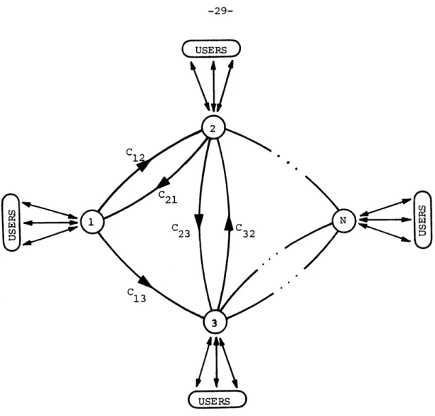
In a network consisting of N nodes we associate with each node an integer in the set {l, 2, ... , N} and denote this collection of nodes by N. The link connecting node i to node k is denoted by (i,k), and the collection of all links in the network is

A

Notation 2.1 L = {(i,k), such that i,k c N and there is a direct link connecting i to k}.

We now denote

Notation 2.2 C. = capacity of link (i,k) in units of traffic/unit time, (i,k) E L

and for every i e N denote

A

Notation 2.3 E(i) = collection of nodes k such that (i,k) E L, I(i) = collection of nodes 2 such that (Mi) E L.

In Figure 2.1 we depict a graphical representation of such a data com-munication network.

\2/

Th

~Cl

Figure 2.1 Data Communication Network Topology

2.2.2 Message Flow and Storage Representation

In accordance with the operational philosophy of the network, the users at each node in the network may input messages whose ultimate destinations are any of the other nodes in the network. We characterize this message traffic flow input to the network by:

Notation 2.4 a (t) = rate of traffic with destination j arriving 1

-30-at node i (from associ-30-ated users) -30-at time t.

The message traffic from each user is first fed into the associated node and either immediately transmitted on an outgoing link or stored for eventual transmission. Also, each node may serve as an intermediate storage area for messages entering on incoming links enroute to their destinations. Once a message reaches its destination node, it is im-mediately forwarded to the appropriate user without further storage.

Hence, at each node i e

N

(i+l), ...N. We now define the state variables of our model as

Notation 2.5 x0(t) = amount of traffic at node i at time t whose final destination is node j, where

iij

N,

j.

The amount of traffic residing in each box at any time t is mea-sured in some arbitrary unit (messages, packets, bits, etc.). Strictly speaking, the states are therefore discrete variables with quantization level determined by the particular unit of traffic selected. However, we shall assume that the units are such that after appropriate

normali-zation the states x. can be approximated by continuous variables. The rationale underlying this approximation is presented in Section 1.2.

We simply repeat here that this macroscopic point of view regarding messages is justifiable in relation to the overall goals of desirable network operation. Note that in a network consisting of N nodes, the maximum number of state variables as defined above is N(N-l), which most certainly is reasonable when compared to the huge number of states

associated with finite-state models (see Section 1.2).

There is a fundamental difference between the states xi described here and the message queues of the traditional approach. In our model, when a message with destination

j

classi-fied as belonging in the "box" x , and as such is associated with the node i. When its time comes to be sent, the routing strategy to be developed in subsequent chapters assigns the message to be sent along some outgoing link (i,k),k E E(i). In previous models (e.g., Cantor and

and Gerla (1974]) messages arriving at node i are immediately assigned to some outgoing link (i,k),k E E(i), by the routing strategy, there to

await transmission. Hence, at least in an intuitive sense, the decision as to what direction to send a message is made in our model at a later time, thus enabling the strategy in force to make a more up-to-date decision. The ultimate performance of our strategy should benefit from

this characteristic.

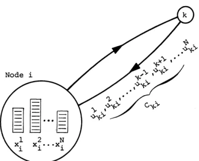
The final element of our message flow representation is the de-scription of the allocation of link flow capacity. Each link emanating from a particular node i is shared by some or all of the up to (N-l)

-32-types of messages stored at time t at node i. This now gives rise to the definition of the control variables of our state space model:

Notation 2.6: uk (t) = portion of the rate capacity of the link (i,k) ik

used at time t for traffic with final destina-tion

j.

So defined, the controls are the decision elements of the model available to be adjusted at the command of the routing strategy. The designation of the states corresponding to a particular node and controls

correspond-ing to a particular link are illustrated in Figure 2.2.

Node i

H

C4-Illustration of State and Control Variables Figure 2.2

2.3 Dynamic Equations and Constraints

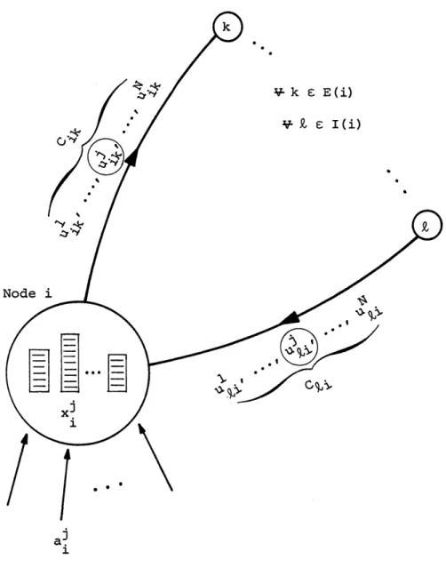
We are now ready to state the dynamic relationship between the elements of our state space model. Assuming the inputs are determin-istic functions of time, the time rate of change of the number of mes-sages contained in each box is given by

x. (t) = a! (t) - , u (t) + u. (t) (2.1)

kEE(i) ik kl

ijj e

N,

That is, the box corresponding to the state x. is increased by the rate 1

of messages arriving from users (al(t)) and messages arriving on

in-j1

coming links (u3 (t), E I(i), /

j)

ik'

depiction of the message flow situation corresponding to equation (2.1) is given in Figure 2.3.

The ordinary differential equation formulation of equation (2.1) is valid for deterministic inputs. When the inputs are stochastic, we must express the relationship in the incremental fashion of stochastic differential equations and properly define the nature of the input pro-cess. However, the important point here is that the state space

de-scription of message flow and storage presented in Section 2.2 is suffi-ciently general to accommodate a wide variety of input processes.

An essential feature of the model is the set of constraints we must impose on the state and control variables. In order for the

-34-V- k s E(i) V 91 I(i) Node

U...

/ /

Figure 2.3 Elements of Message Flow

mathematical statement of our problem to make physical sense, we must insist on non-negativity of the message storage state variables and of the flow control variables:

x1(t) > 0 'V t (2.2)

and

ui (t) > 0 I t. (2.3)

ik

The rate capacity constraints on each transmission link is expressed by

u (t)

< C.

IV t

sN

/

Constraints (2.2)-(2.4) are the only ones which shall be dealt with explicitly in this thesis. The assumption is therefore made that the storage areas containing the messages corresponding to the state vari-ables are infinite in capacity. In practice, of course, these areas will be limited in size, so that we may wish to insist on upper bounding

state variable constraints. Possible forms of these constraints are

x < Si or xj < S. depending on the actual assignment of message 1 -

i

storage in a node.

2.4 Performance Index and Optimal Control Problem Statement

As indicated in Section 1.2, one of the major problems associated with routing strategies predicated upon queueing models is the require-ment of the independence assumption in order to derive the closed-form expression for the total message delay in the network. This assumption

-36-may be at great variance with the physical realities of the situation. On the other hand, optimal control oriented formulations such as ours

require only a functional expression for the quantity of interest in terms of the state and control variables of the model. By design, the method in which we have defined the state variables gives rise to possi-ble performance indices which are most appropriate in this application.

For example, observe that if x(t) is the amount of message traffic residing in some box at time t, then the quantity

ftf

0

gives the total time spent in this box by the traffic passing through it during the time period of interest (t0, t ], when tf is such that x(t f) = 0. Consequently, expression (2.5) is exactly the total delay

in the box experienced by the class of messages represented by x(t). Hence, the total delay experienced by all the messages as they travel

through the network during [t0, t ] is given by

tf

D = x (t) dt (2.6)

t0

irj

N,

where tf is defined as the time at which all the message storage state variables x. go to zero. Priorities can be accommodated in the cost

appro-priate state variables, so that we have

tf - _{. .}

J =

fa:x

[(t)

dt

i , j EN , j i

with tf defined as above. A logical fashion in which to assign priori-ties is by destination, in which case a = a I k,P,

j.

At every time t, given the knowledge of the traffic congestion in the network (x (t), i,j E N, j / i), dynami-cally decide what portion of each link capacity to use for each type of traffic (i.e., assign u (t), (ik) E L,

j

ik

so as to minimize the specified cost functional (i.e., total delay if a! = 1 I i,j, i y

j)

To facilitate the expression of this problem in compact mathemati-cal form, we define the five column vectors - a, x, u, C and a - which

are respectively concatenations of the inputs, state variables, control

-38-n = dimension (a) = dimension (x) = dimension () , m = dimension (u) and

r = dimension (C) = card (L). For a given network topology we define

j

the n X m matrix B as follows: associated with every state variable x. is a row b of B such that

T

b u =- u + U (2.8)

-- ik L Pi

kEE(i) k EI(i)

The matrix B is analogous to the incidence matrix which describes flow in a static network. However, a fundamental distinction from the static flow situation is that we do not require conservation of flow at nodes as we have the capability of message storage in nodes. Note that B is composed entirely of +1's, -l's and O's and that every column of B has at most two non-zero elements. If a particular column has exactly one non-zero entry then it is -1.

Similarly, we define the r x m matrix D: associated with every T

link (i,k) is a row d of D such that T

d u < Cik (2.9)

represents the constraint (2.4). The elements of D are O's and +1's only, and each column has precisely one +1.

We may now compactly express the linear optimal control problem with linear state and control variable inequality constraints which represents the data communication network dynamic message routing

problem previously stated:

Find the set of controls u as a function of time and state

u(t) u(t, x) t E , t ] (2.10)

that will bring the state from a given initial condition x(t₀ = to x(tf) = 0 and minimizes the cost functional

ftf

J [a T x(t)]dt (2.11)

t0

subject to the state dynamics

x(t) = B u(t) + a(t) (2.12)

and constraints on the state and control variables

x(t) > 0 4v t

E

D u < C

(2.14) u > 0.

Note that a(t) must be such that the state is controllable to zero with the available controls. Conditions under which this is true are given for a special case in Section 3.2.2.

2.5 Discussion of the Optimal Control Problem

Before engaging in the details of the solution to (2.10)-(2.14), some discussion regarding the validity of the problem statement is

-40-appropriate. To begin, we have stipulated inputs which are known expli-citly as a function of time, whereas computers certainly operate in a stochastic user demand environment. Secondly, the requirement that all

the storage states go to zero at some final time is not consistent with a network continually receiving input and storing messages in a steady fashion. Also, as pointed out in Section 2.3, we have ignored upper bounds on message storage capacity. Finally, by specifying a feedback function of the type (2.10) we are assuming that total information re-garding storage is available throughout the entire network for controller decisions. In practice, one may wish to consider schemes which allow for the control decision to be made on the basis of local information only, so called distributed control schemes.

With the above drawbacks in mind, we now provide justification for

our approach. We begin by pointing out that none of the assumptions made thus far are inherent in a basic state space model. These have

simply been invoked to provide a problem formulation for which there exists some hope of obtaining a reasonable solution at this early stage of experience with the model. Also, they may not be as limiting as they first appear. For instance, one possible approximation for the situation with stochastic inputs is to take into account only the en-semble average rates of the inputs. We then design the routing strategy by solving (2.10)-(2.14) with these averages serving as the

determinis-tic inputs a(t), and employ the controls thus obtained in the operation of the network. Such a strategy may prove to be reasonably successful

if the variances and higher moments of the distributions of the inputs are small compared to the means.

Next, the requirement that all states go to zero at the final time may correspond to a situation in which one wishes to dispose of message backlogs at the nodes for the purpose of temporarily relieving conges-tion in the network locally in time. This procedure may represent that portion of an overall scheme during which inputs are appropriately

regu-lated or no longer forthcoming. In the latter case we may refer to the resulting operation as a "minimum delay close down procedure".

Elimination of the state variable upper bounds is not always

limiting, as we shall discover for a class of single destination network problems studied in Chapter 4. In this case, the optimal routing strat-egy never requires any state to exceed its initially specified value, which certainly must be within the available storage capacity.

Finally, the assumption of a centralized controller may well be valid in the case of a small network. An example of this is the IBM/440 network. See Rustin [1972]. At any rate, obtaining the routing strat-egy under this assumption could prove extremely useful in the determina-tion of the suboptimality of certain decentralized schemes.

2.6 Previous Work on Optimal Control Problems with State Variable

Inequality Constraints

Pioneering research into the problem of the optimal control of dynamical systems involving inequality constraints on the control vari-ables was performed by Valentine [1937] and McShane (1939]. Problems

-42-also involving inequality constraints on functions of the state varia-bles alone were not treated until the early 1960's, probably motivated by the emerging aerospace problems of that time. Pontryagin [19591

provided the setting for the new approaches with the introduction of his famous maximum principle, a landmark work in the field of optimal control. Gamkrelidze [1960] studied the situation in which the first time derivative of the state constraint function is an explicit function of the control variable, or so called "first order state variable

in-equality constraints." Note from equations (2.12) and (2.13) that this is our situation. This work was devoted to finding necessary conditions in the form of multiplier rules which must be satisfied by extremal trajectories. Berkovitz [1962] and Dreyfus [1962] derive similar re-sults from the points of view of the calculus of variations and dynamic programming respectively.

Subsequent works involved with necessary conditions have been devoted primarily to unravelling the technical difficulties which arise when a time derivative higher than the first is required to involve the control variable explicitly (e.g. Bryson, Denham and Dreyfus [1963], Speyer [1968] and Jacobson, Lele and Speyer [1971]). The literature is quite often at variance with regard to the necessary conditions

asso-ciated with this problem, although the later work cited appears to pre-sent a satisfactory resolution. At any rate, we shall not be concerned with these differences as our problem involves only first order state

Computational aspects of the problem are dealt with in Ho and Bretani [1963] and Denham and Bryson [1964]. Both works present itera-tive numerical algorithms for the solution of the open loop problem, the procedure discussed in the latter being essentially an extension of the steepest-ascent method commonly used in control problems uncon-strained in the state. As such, it appears doubtful that this algorithm would exhibit acceptable convergence properties for our linear cost problem, particularly in the vicinity of the optimum. Ho and Bretani

[1963] report that this is also true of their algorithm.

Little theoretical and computationally oriented attention has been paid to the class of control problems with state variable inequality

constraints and control appearing linearly in the dynamics and perfor-mance index. In this case, the control is of the bang-bang type and

the costates may be characterized by a high degree of nonuniqueness. Maurer [1975] examines the necessary conditions associated with this problem when the control and state constraint are both scalars, and presents an interesting analogy between the junction conditions

asso-ciated with state boundary arcs and singular control arcs. However, no computational algorithm is reported.

Perhaps the most interesting computational approach presented for the all linear problem is the mathematical programming oriented cutting plane algorithm of Kapur and Van Slyke [1970]. The basic algorithm con-sists of solving a sequence of succeedingly higher dimensional optimal control problems without state space constraints. Under certain

hypo-

-44-theses they are able to prove strong convergence of the control to the optimum. The drawbacks to this approach are that the state of the augmented problem may grow unreasonably large, and that even uncon-strained state linear optimal control problems may be difficult to solve efficiently. In the same paper Kapur and Van Slyke [1970] suggest for-mulating the problem as a large linear program through discretization of all constraints, a more or less brute force approach which is

dis-cussed briefly in Section 2.7.1.

Common to all of the approaches described above is that none broach the difficult problem of obtaining feedback solutions to the

state constrained optimal control problem. In fact, the application of necessary conditions to arrive at feedback solutions is not a common occurrence even for unconstrained state problems. Notable exceptions are the linear time-optimal and linear quadratic problem, for which the feedback solutions are well known.

In light of these facts, in order to solve problem (2.10)-(2.14), we must first develop and understand the necessary conditions associated with optimal solutions and creatively apply them to obtain a feedback solution. Certainly, we must fully exploit the total linearity of our problem, which has not been done heretofore. As is usually the case, we shall be forced into making even further assumptions about the

prob-lem in order to achieve our goal. This overall effort constitutes the primary mathematical contribution of this work, and is the subject of

2.7 Open Loop Solutions

Although our foremost goal is the development of feedback solu-tions to the optimal control problem of Section 2.4., several open loop

solutions have received consideration. The principal advantage of these approaches is that they apply to inputs represented by determin-istic functions of time of arbitrary form. Also, at least in principle, open-loop solutions may be implemented as feedback schemes by continu-ally recalculating them in time with the current state taken as the initial condition for each problem. As such, open-loop solutions are worthy of brief mention at this time, but we shall not pursue these particular approaches further in this thesis.

2.7.1 Linear Programming Through Discretization

This technique is a rather standard approach for linear optimal control problems. See, for example, Kapur and Van Slyke [1970). We first begin with the assumption that the inputs are such that the state can be driven to zero with the available controls. Next, we select a time T which is sufficiently large to insure that T > tf, where t is such that x(t f) = 0. To discretize, we divide the time interval [0, T] into P parts, each of length At = tP-tp-i, p 6 [l, 2, ... , P]. We then make the Cauchy-Euler approximation to the dynamics

x(t ) = [x(t ) - x(t )]/At. (2.15)

- p - p+1 - p

-46-x(t ) = x(t ) + At[a(t ) + B u(t )], (2.16)

- p+1 -p -p p

VL p E :0, 1, ... , P-l]

and the performance index may be approximated to first order by the discrete expression

P

S=

E

d - p

p=0

In this format we have the following constraints:

D u(t ) < C (2.18a) -_ p - -u(t ) > 0 (2.18b) - p - -x(t ) > 0 (2.18c) -

p--VP

We now consider the x(t ) and u(t ) IV p e [0, 1, ... , P] to be

- p - p

the decision variables of a linear programming problem. The total number of such variables is (n+m)P. The non-negativity constraints

(2.18b) and (2.18c) are consistent with standard linear programming format.

Since (2.17) is a linear function of the decision variables, we have a linear programming problem with nP equality constraints (2.16)

and rP inequality constraints (2.18a). The general format of the program is known as the "staircase structure", a form which has re-ceived considerable attention in the programming literature. Such works are devoted to exploiting the special structure of the problem in

order to reduce computation through application of decomposition

tech-niques. See, for example, Manne and Ho [1974]. Cullum [1969] proves

that as the number of discretization points P goes to infinity, the solution to the discrete problem approaches the optimal solution of the original problem. However, for a reasonable size network and for P sufficiently large to insure good quality of the approximation, the size of the linear program (both in terms of the number of variables and the number of constraints) becomes prohibitively large for practical appli-cation. For this reason, this technique has been applied only for the purpose of obtaining sample solutions to provide insight into the pro-perties of optimal solutions.

2.7.2 Penalty Function Method

Optimal control problems with inequality constraints on the state (and/or) control have frequently been solved in an open-loop fashion by converting them to a sequence of problems without inequality constraints by means of penalty functions. One such technique is presented by

Las-don, Warren and Rice [1967]. The penalty function detailed in that paper works from inside the constraint, the penalty increasing as the

boundary is approached. Applying this technique to our situation, the

state variable inequality constrained problem (2.10)-(2.14) is converted to a problem without state constraints by augmenting the performance index with a penalty function as follows:

-48-T J =(x (t) + E3/x (t)) dt (2.19) a . . 1i j> 0 1

irj

N,

j.

The modified problem is then to minimize (2.19) subject to the dynamics (2.12) and the control constraints (2.14).

Since the penalty function term

f (E /x (t)).dt] ij c N, i 0

j

0o i,) i

approaches infinity as any x approaches its boundary x = 0, we would speculate that the minimizing solution remains within the constrained region x > 0. In Lasdon, Warren and Rice [1967] it is shown that this

conjecture is true, and further that the minimizing control as a func-tion of time and the minimizing cost approach those for the constrained

problem as max

(s)

approach-i,j

ing the constraint boundary from the interior, any solution for the unconstrained problem is also feasible for the constrained problem.

In order to implement this technique, we need to solve the uncon-strained problem by any appropriate numerical technique for successively decreasing values of E . Gershwin [1976] has created a program for the solution of the penalty function approach to this problem in which he utilizes a modified form of differential dynamic programming for each

unconstrained minimization. The computational efficiency of the al-gorithm is greatly enhanced by the exploitation of parametric linear programming techniques. Whether or not this scheme encounters numerical

difficulties as E. grows very small remains to be determined. 1

Chapter 3

FEEDBACK SOLUTION TO THE OPTIMAL CONTROL PROBLEM WITH CONSTANT INPUTS

3.1 Introduction

We have formulated the data communication network dynamic message routing problem as the linear optimal control problem of Section 2.4.

In this chapter we develop the fundamental theory underlying a novel approach to the synthesis of a feedback solution to that problem. The

technique is predicated upon the assumption that all inputs to the net-work are constant in time. In this section we present a brief review

of the development.

We begin by presenting the necessary conditions for the general deterministic problem (inputs not constrained to be constant) and dis-cuss these conditions in some detail. We then show that these condi-tions are also sufficient, a most fortuitous situation since it guaran-tees the optimality of trajectories which we eventually shall construct using these conditions.

The subsequent discussion is restricted to the constant inputs case. Based exclusively on the necessary and sufficiency conditions, a geometrical characterization of the feedback space for constant inputs is presented: the regions of x-space over which the same controls and

-50-sequence of states on and off boundary arcs are optimal are convex poly-hedral cones in the state space. It is this special property (a result of the total linearity of the problem) which embodies the adaptability of the constant input formulation to the synthesis of a feedback solu-tion. What one needs is an algorithm to specify these regions and the

appropriate controls.

Next, we present several simple examples to illustrate how these regions may be constructed. This is accomplished by producing a certain set of optimal trajectories backward in time from the final state x = 0. Each portion of these trajectories generates one of these convex poly-hedral conical regions, thereby providing the optimal control in that

region. If a sufficiently complete set of trajectories is calculated, we manage to find enough regions to fill out the entire space.

The remainder of the chapter is devoted to the extension of this concept to the general network optimal control problem with constant inputs. Taking the lead from the examples performed, an

algor-ithm is presented for the construction of the conical regions from a comprehensive set of backward optimal trajectories. This algorithm is in general form, and several specific issues are raised regarding its execution. An issue of central importance is the determination of the appropriate set of costates required by the algorithm. The resolution of this question is essentially geometrical in nature, relying upon the interpretation of the Hamiltonian as a continuously rotating hyperplane. In fact, many of the arguments are geometrical, so that we frequently