Analyzing tradeoffs between working capital and production capacity for multi-stage manufacturing processes

(1)

Analyzing Tradeoffs between Working Capital

and Production Capacity for Multi-Stage Manufacturing Processes by

Karim Kamareddine

Bachelor of Science, Mechanical Engineering, University of Massachusetts Amherst, 2012 and

Yihong Yao

Bachelor of Management, Business Administration, Shanghai Jiaotong University, 2013

SUBMITTED TO THE PROGRAM IN SUPPLY CHAIN MANAGEMENT IN PARTIAL FULFILLMENT OF THE REQUIREMENTS FOR THE DEGREE OF

MASTER OF ENGINEERING IN LOGISTICS AT THE

MASSACHUSETTS INSTITUTE OF TECHNOLOGY JUNE 2016

The authors hereby grant to MIT permission to reproduce and to distribute publicly paper and electronic copies of this thesis document in whole or in part in any medium now known or hereafter created.

Signature redacted

Signature of A utho r ... ...

Master of Engineering in Logistics Program

Signature of Author...Signature

redacted

May 11, 2016

Mast ,0r-6ngineering in Logistics Program May 11, 2016

Signature redacted_

11 201

Certified by ... ... ...---Dr. Jarrod Goentzel

Director, MIT}Iumanitarian Response Lab

Ar Thesis Supervisor

Signature redactedThssSprio

A cce pted by... ...

7,

U Dr. Yossi Sheffi

irector, Center for Transportation and Logistics

Elisha Gray 11 Professor of Engineering Systems MASSACHUSETTS INSTITUTE Professor, Civil and Environmental Engineering

OF TECHNOLOGY

JUN 3 0

2016

LIBRARIES

Abstract

Large pharmaceutical companies struggle to find innovative ways to reduce work-in-process inventory in their production facilities. In our research, we focus on the tradeoff between inventory and production capacity through investing in new facilities and equipment. This tradeoff will depend on the company's objectives and what it is willing to give up in return for reducing inventory. We found that increasing capacity to reduce work-in-process inventory by investing in new facilities is not always the most favorable approach in terms of net present value. However, for flexibility or lead-time improvements, it may make sense to proceed with the investment. We developed multiple scenarios considering the company's future plans to reduce inventory or grow. These scenarios provide insights into the factors that improve the attractiveness of the investments and those that do not. Our financial analysis along with the guidelines and procedures that we have developed help the sponsor company most effectively reach its goal to reduce its work in process inventory.

Thesis Supervisor: Dr. Jarrod Goentzel

(3)

Biographical Notes

Karim Kamareddine grew up overseas in Lebanon. After high school, he attended college in Massachusetts. He has experience working in the Global Supply Chain of Pratt & Whitney, an aerospace manufacturer headquartered in Connecticut. He has experience in Supplier Quality, Procurement, Materials Required Planning and Strategic Sourcing. He holds a Bachelor of Science in Mechanical Engineering from the University of Massachusetts Amherst. Upon graduation from MIT, he will join Bayer Business Services as a Senior Consultant with a concentration in Management Consulting, Supply Chain Management and Technical Operations.

Yihong Yao is originally from China. She holds a Bachelor of Management in Business Administration - Logistics Management from Shanghai Jiao Tong University. Before MIT, she joined the supply chain leadership program in Danone Baby Nutrition and then worked as a buyer in Akzonobel Swire Paints in Shanghai. She has experience in Planning, Logistics, and Procurement. Upon graduation from MIT, she will join the Hershey's Company as Manager of Supply Chain Learning Academy.

(4)

Acknowledgements

We would like to thank the following people for their contributions to our research: " Jarrod Goentzel for his support, insight and helpful feedback as we wrote our

thesis paper.

" Pamela Siska and Jeanne Marie Wildman for their patience and thorough review of our writing.

" The entire team at the Sponsor Company' and their partners for their generous support and guidance.

" Our families and friends for their endless support and encouragement.

1The word 'sponsor company' has been repeatedly used throughout the paper to maintain the

(5)

LIST OF FIGURES

Figure 1: Typical pharmaceutical supply chain (Sundaramoorthy & Karimi, 2004) ... 12

Figure 2: Gated Process for Investing (Uwe G6tze, Deryl Northcott, Peter Schuster, 2007)...15

Figure 3: API Production process (Arul Sundaramoorthy, Xiang Li, James M.B. Evans, Paul 1. B a rt o na, 20 12 ) ... 19

Figure 4: Production schedule for one large module (base scenario)... 20

Figure 5: Production schedule for first small module (base scenario)... 21

Figure 6: Production schedule for second small module (base scenario)... 21

Figure 7: Stock profile of one m odule ... 23

Figure 8: Stock profile for two smaller modules investment ... 24

Figure 9: Free Cash Flow Analysis for the One Module Baseline Scenario... 27

Figure 10: Scenario Assum ption Sum m ary... 29

Figure 11: Production schedule for scenario 2 - first module ... 30

Figure 12: Production schedule for scenario 2 - second module ... 30

Figure 13: Production schedule for scenario 3 - first module ... 30

Figure 14: Production schedule for scenario 3 - second module ... 30

Figure 15: Causal loop diagram of the production system... 37

(8)

LIST OF TABLES

Table 1: Calculation the Cost of Goods Sold as a percentage of Revenues... 18 Table 2: Four-stage production process KPI Results... 32 Table 3: Two-stage production process KPI Results ... 33

(9)

1. Introduction

Our thesis examines the tradeoff between net working capital and the capital investment of a major pharmaceutical company. First, we provide an overview of the challenges facing pharmaceutical companies, then break down the different cost elements needed to make specific supply chain investments and finally determine effective supply chain outcomes under different scenarios that consist of multiple stages and different changeover frequencies. This analysis provides us with tremendous insights into how different parameters can affect the outcomes of the different scenarios and ultimately the key performance indicators (KPI's) that the pharmaceutical company would like to focus on.

The production process for the pharmaceutical product in question is carried out in four stages where raw materials are converted into Active Pharmaceutical Ingredients (API's) sequentially. The output work in process inventory of each stage is the input of the next stage and there is considerable wasted time changing over from one stage to the next. We tend to study this production process in a very simplified approach by looking at the production schedule of one anonymized product at first and consequently analyzing how the work in process inventory of this product can be reduced while still maintaining an effective production process. This same analysis is also done for different multi-stage processes.

Our sponsor company's objective for this year is to reduce work in process inventory, so we have provided different investment scenarios that attempt to reduce this inventory while still maintaining a high return on investment. In an attempt to reduce net working capital, increase free cash flow and generate more profits, our sponsor company has asked us to provide guidelines and procedures to balance working capital and capital investment. Our thesis paper provides a quantitative analysis of specific investment scenarios to be used by key stakeholders at the sponsor company to evaluate options. The quantitative analysis is supplemented with reasoning that helps guide stakeholders to make informed decisions.

We used financial factors in our supply chain analysis to determine the tradeoff between capital investment and working capital with the primary objective of maximizing the net present value (NPV). We do this by first asking the sponsor company for the cost breakdown of a specific investment, calculating the free cash flows and the NPV of each investment, and then comparing different scenarios using Key Performance Indicators

(KPI's).

In our paper, we consider a module to be the production facility that houses all the production equipment needed to create a finished product. We begin our analysis by examining a few simple scenarios and later expand the analysis by providing

(10)

supplementary scenarios that would provide the sponsor company with various real-life situations that they may encounter. We first examine a base scenario that includes a one module investment and a two-module investment. The one module investment is comprised of a 4-stage production process and requires 4 changeovers per year. The two-module investment is also comprised of 4 stages per two-module and requires a total of 12 changeovers per year. Refer to Appendix A for further details about the production schedule.

It is very important to evaluate exactly how these investments will impact our sponsor company's key performance indicators. Financial analysis will be key to understanding the effectiveness and feasibility of the investments. Finally, we provide the sponsor company with options to consider, depending on their main objective.

In our case, future demand is assumed to be constant and certain. The sponsor carries significant finished goods safety stock to provide good service in spite of variable demand and requested that the analysis focus on work in process inventory. We do point to opportunities to reduce finished goods safety stock as future work.

Some of the guidelines that we have provided to the sponsor company highlight the reasons to build one or many modules while mentioning some of the considerations that the company should not overlook. We also provide analysis highlighting key elements that may impact whether the company should pursue an investment such as: flexibility, risk, and adaptability.

We use financial analysis in conjunction with these other factors in considering tradeoffs among key performance indicators. We also develop several scenarios to evaluate tradeoffs between working capital and production capacity investments.

2. Literature Review

This section highlights focuses on supply chains in the pharmaceutical industry by referencing literature and discusses some the key elements that need to be outlined when making an investment decision.

2.1 The challenges

Pharmaceutical companies are facing rising challenges. Overall speaking, the pharmaceutical industry is becoming more liberalized on a global scale (Shah, 2004). The resulting competition along with more stringent regulatory control impel companies to increase profitability.

While traditionally companies place much emphasis on research and development (R&D) and charge a substantial premium for products to generate revenue, the

(11)

productivity of R&D is generally decreasing. To make things worse, the life cycles of new drugs are declining (Papageorgiou, Rotstein, & Shah, 2001). The new products, which normally take companies years to develop, not only face the uncertainty of clinical tests, but also the challenge of generic substitutes from competitors.

Faced with all these challenges, supply chain optimization is gaining prevalence as an excellent way to increase profitability. The diversity and complexity of new drugs, shortening life cycles, the globalization of the business which requires managing global manufacturing and supply networks all requires supreme supply chain management and optimization (Papageorgiou et al., 2001).

2.2 Pharmaceutical Supply Chain Characteristics 2.2.1 Overall Introduction of Supply Chain Layer

Sundaramoorthy and Karimi proposed that most pharmaceutical supply chains feature a layer structure as illustrated in Figure 1 (Sundaramoorthy & Karimi, 2004).

Layer 1. In the first layer, companies interact with suppliers that provide raw materials and/or intermediates to the primary and/or secondary production sites and third-party contractors that supply intermediates.

Layer 2. This layer involves the primary production sites that produce active ingredient

(API) using chemical or biochemical technology such as chemical synthesis, separations, fermentation, purification, etc. The input of this layer is raw materials and/or intermediates and the output are the API's.

Layer 3. This layer involves secondary manufacturing sites where the API's are

transformed into a medicine that the patient can take, such as a tablet, capsule, syrup, injection, cream and ointment.

(12)

Layer Suppliers

Outsourced Raw Oumsnurced

Als Mutcin Intermediates

, mer2 2.2.ary Production ;Aclivc Ingredients S c h Secondary Poduction r inish ed Products Layer 4 Warehouses,, Wholesalers ' Retailers ' Lnd-l scrs

Figure 1: Typica1 pharmaceutical supply chain (Sundaramoorthy & Korimi, 2004)

2.2.2 Primary Manufacturing

Shah described the primary manufacturing process as one with long task processing times,

multi stages and substantial inventories (Shah, 2004). This is due to the stringent requirements for validating cleaning and purity and the need for avoiding cross-contamination in the pharmaceutical industry (Sundaramoorthy & Karimi, 2004). In order to increase utilization of facilities, primary manufacturing often features long campaigns to minimize changeover. As a result, the traditional single-facility, long-campaign production yields considerable inventory at each stage and less responsiveness to market demand.

2.3 Optimization in Different Scenarios

In this section, we review literature that discusses supply chain optimization in different scenarios. The first two scenarios are most similar to our base model.

2.3.1 Multi-site and Multi-product

Kallrath developed a multi-site, multi-product, multi-period production network planning model for BASF with the objective of determining the production schedule given a certain demand (Kallrath, 2000). Grunow, GUnther and Yang discussed the coordination

(13)

among multiple sites and the campaign schedules at different sites with a certain demand and tackled the problem using an innovative mixed-integer linear programming (MILP) model (Grunow, Ginther, & Yang, 2003).

2.3.2 Incorporating Financial Considerations

Puigjaner and Lainez proposed a scenario-based multi-stage MILP model to maximize corporate value by combining financial factors with supply chain indicators (Puigjaner & Lainez, 2008).

2.3.3 Uncertain Demand

Verderame, Elia, Li and Floudas reviewed planning and scheduling under uncertainty (Verderame, Elia, Li, & Floudas, 2010). Two-stage stochastic programming, parametric programming, fuzzy programming, chance constraint programming, robust optimization techniques are common tools to approach optimization problems.

2.3.4 New Product

R&D in the pharmaceutical industry is exposed to greater risks compared with other industries. The uncertainty in clinical trial outcomes needs to be built into the optimization model of new products. Levis and Papageorgious came out with a systematic mathematical programming approach for long- term, multi-site capacity planning with uncertainty in the pharmaceutical industry (Levis & Papageorgiou, 2004). They developed a two-stage, multi-scenario, MILP model and adopted a hierarchical algorithm to reduce the computational effort needed to solve the MILP model.

2.3.5 Different tax rates

Oh and Karimi illustrated the influence of regulations (corporate taxes, import duties and duty drawbacks) on the linear programming (LP) model to approach production-distribution planning problem (Oh & Karimi, 2004).

2.4 Investments Types

According to G6tze, Northcott, and Schuster (2007), there are three main types of investments: Foundational, Current and Supplementary. Foundational investments are linked with a start-up and they can either be investments in a new company or in an existing company's branch at a new location. Current investments are replacement, major repair or general overhaul investments. Supplementary Investments refer to investments in equipment in existing locations and they can be classified as expansion, change or certainty investments. Our investment focuses mainly on the supplementary category.

2.5 The Investment Motive

Typically, the motive behind an investment can either be operational, strategic or financial and any company that decides to invest has a specific goal in mind that it would

(14)

like to attain. Quantitative methods and, in particular, mathematical programming models, have traditionally been used to make investment decisions at tactical or operational levels. However, mathematical models can and should also be used to address strategic decisions because these have a much greater impact on the results (Martinez-Costa, Mas-Machuca, Benedito, Corominas, 2014). Operationally, the company can be making the investments for the purposes of procurement, sales, administration, or research and development (Uwe G6tze, Deryl Northcott, Peter Schuster, 2007). The investment will most likely have the biggest impact on the supply chain of the company but as G6tze, Northcott, Schuster, (2007) stated, many investments that are instigated by one operational area affect other parts or decisions of the company.

Consider the decision to invest in a second module in a nearby location. The procurement of this long-term asset is primarily decided using assumptions about future production requirements. However, an expansion carried out to manufacture a new product type, for example, is an interdependent investment project, requiring considerable coordination of decisions from areas like sales, production, financing, human resources and research and development (Uwe G6tze, Deryl Northcott, Peter Schuster, 2007). Therefore it is important to understand which stakeholders will be affected by these decisions in order to receive the appropriate buy-in from the entire organization.

2.6 Investment Uncertainty

It is important to mention that, with any investment, there is a level of uncertainty that needs to be accounted for (Uwe G6tze, Deryl Northcott, Peter Schuster, 2007). There typically are not any investments that have certain or known effects since investments take place over a period of time rather than instantaneously. However, there are different levels of uncertainty and some investments can have effects that are more or less certain depending on the complexity of the investment. We can plan for certain disruptions; however, not everything can be anticipated. Bienstock and Shapiro (1988) for example advise that there are uncertainties in the external environment that are relative to prices, capital markets, government policies and competition that there is no control over.

2.7 Financial Analysis

The company's strategy could include a gated process (see Figure 2) whereby different decisions will be made at each gate in the process that hopefully align with the company's goals, ruling out projects or ideas that are not worth investing time and energy in. The gated process is displayed in Figure 2 below. Ultimately, the NPV analysis can provide us with a framework to make our decisions but should also be supplemented with qualitative analysis of the investment decision.

(15)

"I) Ltltt DIe not: mn(sthtLg

14-3. irc & icNci posisitic roct

4-I" F

-I

7.Moior a-nd post audit prqjwc.

Iiiedback &

Figure 2: Gated Process for Investing (Uwe Gbtze, Deryl Northcott, Peter Schuster, 2007)

2.8 Capacity Planning of a Multi-Module System

Some benefits to building a secondary module can be related to strategic capacity planning. In the case of multi-site problems, there are two options: capacity expansion without new site installation and capacity expansion with new site installation as was mentioned by Chen et al., (2013). The former includes the detail of bottleneck machines or tools purchase decisions at a particular site. The latter problem involves decisions such as when and with what capacities new plants should be constructed. This confirms that one of the key challenges that decision makers routinely encounter is to ensure the availability of enough production capacity to meet the demands of products through efficient capacity planning (Arul Sundaramoorthy, Xiang Li, James M.B. Evans, Paul 1. Barton, 2012).

2.9 Evaluating Risk

Fox, Birt, James, Kokko, Salverson and Soflin (2009) mention that shortages in material may occur, which is another form of risk that pharmaceutical companies need to have full control over and visibility into. Shortages occur as a result of raw material unavailability, manufacturing/regulatory issues, inventory practices, unexpected

(16)

increases/shifts in demand, and natural disasters. According to Swaminathan (2002), risks associated with making any decision need to be reduced. One way of doing this is to make sure that there are constraints that limit the amount of shortages.

2.10 Impacts on Inventory

A major dilemma resides in determining the optimal level of buffer stocks to

adopt which allows a reduction of the total incurred cost and ensures a high level of customer satisfaction (Assid, Gharbi, Dhouib, 2015).An investment that can reduce inventory becomes a lot more attractive; however, there is a tradeoff between managing inventory levels and maintaining an optimized supply chain. Pharmaceutical companies are continually seeking to improve the planning and control of the supply chain as well as the efficiency of their production process as Assid, Gharbi, and Dhouib (2015) mention.

2.11 Summary

The bulk of our research and analysis will involve analyzing different investments through NPV analysis and studying different scenarios of the investment by adjusting our input parameters. The literature just referenced will supplement the quantitative analysis that we will provide and will reiterate the importance of analyzing the broader spectrum of factors that may or may not be influenced by the investment decision. At the initial stages of the study, the analysis is performed at a low level and at the final stages, we will introduce additional parameters that may influence investment decisions differently.

In summary, this literature demonstrates the importance of having qualitative analysis that can supplement the quantitative analysis that we will present in the data analysis and results section of this thesis paper. A great deal of research has been done to discuss whether investment decisions are feasible through MILP analysis. Our sponsor company prefers to have guidelines and procedures supplement such quantitative analysis in order to consider internal customers and stakeholders. Next, we will explore the specific case study of our sponsor company.

3. Data Collection

This section describes the data collection necessary to answer the questions posed the sponsor company. We initiated data gathering with formal meetings with the sponsor to better understand the cost breakdown of their operations and their expectations of the thesis project. For instance, we inquired about the typical COGS, labor costs, operating costs, capital and equipment costs that any production module incurs. The

(17)

breakdown of the cost elements that were studied were listed below. See Appendix C for details on cost breakdown that was discussed with the sponsor company.

Direct Labor: The direct labor in this case is the labor cost associated with the hourly wages of employees producing the material in the different stages of production. The salary for the direct labor force ranges between E50K and E110K and the number of employed salary workers is about 8 employees per module. In our analysis, the annual salary is estimated to be E60K.

Material Cost: The material cost is used for inventory valuation. It begins with the cost to procure raw material from suppliers and increases in each of the four different stages of production as variable costs accumulate. For example, in Stage 1, the cost increases from E400/kg to E450/kg. In stage 2, the cost increases from E450/kg to E500/kg. In stage 3, the cost increases from E500/kg to E550/kg. Finally, in stage 4, the cost increases from E550/kg to E600/kg.

Fixed Overhead: The fixed overhead cost includes indirect labor, distribution, waste

management and repair and maintenance. The indirect labor is associated mainly with management as well as personnel that is responsible for the changeover from one production stage to the next. The personnel include: production supervisors and quality control staff. Total fixed overhead is estimated to be between E700K and E1.5 million. In our analysis, the fixed overhead is estimated to be E960K per module.

Variable Overhead: The variable overhead includes energy, consumables and overtime. It is estimated to be between E300K and E3 million. In our analysis, the variable overhead is set at E300K.

Operating Expenses: The operating expenses cost element is the sum of the variable

overhead and fixed overhead cost.

Equipment Cost: Production equipment that has a capacity of 5 tons per week was assumed to cost f30M. This was the equipment necessary to produce the finished goods for the base scenario. In our analysis, we assumed that the equipment cost is proportional to the capacity. For example, if the capacity was 4 tons per week, then the equipment cost would be E24M. Finally, the equipment was assumed to have a life of 10 years.

Module Cost: The module cost was f1OM which was equitable to the cost of the primary facility. The module was assumed to have a life of 40 years.

Discount & Tax rate: The discount rate is 9% and the tax rate is 20%.

Depreciation: We assumed a straight-line depreciation method for the equipment that was used in the facility over 10 years.

Inventory: The inventory value was calculated to be the average of the weekly inventory levels. In other words, the general equation used to calculate the inventory value is:

(18)

Inventory value = E(average weekly inventory values)

52 weeks/year

The total average inventory cost for one module was calculated to be 8.24M (See Appendix D for details). The same analysis was done for the two-module scenario. The inventory was calculated to be E4.28M, a reduction of approximately 48%.

Inventory Holding Cost: The cost of capital for inventory was implicitly included in the free cash flow analysis. Other components of inventory holding cost were assumed to be negligible as the company owns the warehouse space and believes the holding cost will not be of concern.

Changeover cost: The changeover cost was not provided to us as it was difficult for the sponsor company to quantify exactly what the cost would be. Instead, we assume that he changeover cost is directly correlated to the initial equipment cost. Please refer to section 4 for details.

Accounts Payable and Accounts Receivable: The accounts payable and accounts receivable were disregarded for the purposes of this analysis and were not used when analyzing working capital. This was discussed and agreed upon with the sponsor company. Revenues: Revenues were calculated with the help of the financial statements of the company. Over a period of 3 years between 2012 and 2014, the COGS of the company averaged to be 24% of the revenues, yielding a 76% gross margin. Since we knew the

COGS of the product considered in this case, we assumed that the revenues would be

COGS/0.24, which in this case was calculated to be E88M. Please refer to Table 1 for

details.

Year 2012 2013 2014

COGS/Revenues 23.06% 24.96% 24.10%

Table 1: Calculation the Cost of Goods Sold as a percentage of Revenues

The revenues for the two smaller modules were assumed to be equal to the revenues of the large module since the two smaller modules produce the same tonnage at the end of the year. We assumed that finished products that were produced in Stage 4 were sold at a certain and constant rate of 1 ton/week or 52 tons/year. We assumed this in order to simplify our analysis.

(19)

4. Methodology and Approach

This section of the paper discusses how analyzed the data that were given to us along with the questions that we asked ourselves as we explored the data. The first part of this section looks at the two different investments: (1) One large module investment (2) Two smaller modules investment. The second part explains the methodology we used to analyze the data. In section 5 of this paper we use this methodology to find results and use them to propose recommendations in section 6. We used net present value as a primary metric to identify whether one opportunity was more attractive than the other. We looked pros and cons of making either investment. Finally, we proposed different scenarios to study how different situations affect key performance indicators.

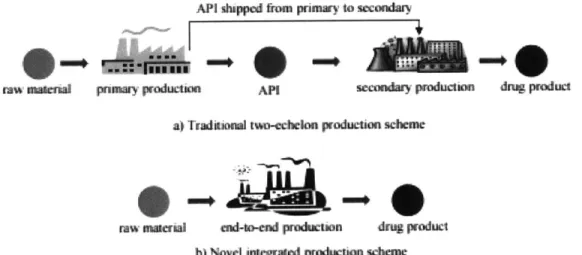
At first, we had multiple discussions with the sponsor company to distill the exact resources that would be needed to invest in the new module. Initially, we came to understand that our sponsor company's pharmaceutical production line is comprised of four key stages. Each stage of production cannot be initiated before the prior stage is complete. Traditionally, pharmaceutical manufacturing is composed of primary manufacturing facilities where raw materials are converted into active pharmaceutical ingredients and of secondary manufacturing facilities where the active pharmaceutical ingredients are developed into the finished products. More recently, pharmaceutical companies, including our sponsor company, have made the switch to continuous manufacturing where raw materials are converted into active pharmaceutical ingredients and finally into the finished products, all in one facility. This allows for a more efficient manufacturing process and hence a more efficient supply chain. The production process is illustrated in Figure 3:

AIP shipped fron pnimarv to scoondarm

ra tanrul prumar prdIAUICLKI API SeCdaN produLcik.n dnug produt

j i I ~ILIOCMI 1V4-CCIhe ILMl (idUe fti SC hmfh

.a

au r cuna to-c" prodK) i heme L

b i Novel inwegf ad prodution -cheme

Figure 3: API Production process (Arul Sundoromoorthy, Xiang Li, James M.B. Evans, Paul I. Bartona, 2012)

With the help of the sponsor company, we were able to identify what an investment in a new module would entail. There are a few assumptions that needed to

(20)

be considered when breaking down the cost. First, we assumed that the investment was going to be located near the primary facility. This means that the tax rate and discount rate remain the same. This also means that transportation cost from one facility to the incumbent facility will be small relative to the total cost, so we assumed it to be negligible. The transportation here is referring to the movement of goods from one facility to another. For example, if Stage 1 was complete in the primary facility and management decided there was not enough capacity in one module, the material would be transported to the second module in order to produce Stage 2. This will be done to reduce lead-time of the finished product and to increase production flexibility, which will be discussed in section 5.7.

The second assumption is that the number of direct labor employees needed for a large module is 8. On the other hand, the number of direct labor employees needed for two small modules is 16, double the number of employees in the large module investment. On that same note, the number of indirect labor employees at one large module is 8 and is the same for two small modules.

The third assumption was that the fixed overhead is proportional to the number of modules, and thus the fixed overhead of two modules doubles that of one module. However, for both the large module and two smaller modules, the variable overhead cost remains the same since the total volume produced is constant.

4.1 Production Scheduling

For the base scenario, the production schedule information was provided to us by the sponsor company.

The production runs that are needed to for the one large module investment can be found in Figure 4 below:

C/o C/o C/o C/o

stage 1 2 3 4

Quarter Q1 02 Q3 Q4

Figure 4: Production schedule for one large module (base scenario)

The raw material is delivered to the production facility and in Q1, Stage 1 begins to be produced. After the completion of the stage 1 material production, a changeover process occurs (C/O), at which point the facility is prepared for the second stage. The changeover process takes about 2 weeks on average and there are 4 changeovers per year. Stage 2 material is produced in Q2, Stage 3 in Q3 and Stage 4 in Q4. The next year, the same cycle is initiated all over again. According to the sponsor company, this creates large batch sizes and little room for flexibility. In other words, if in Q1, the customer needed finished product, assuming there was no inventory of finished product in-house,

(21)

the lead-time for the finished product would be 39 weeks starting from Raw Material. This calculation will be explained in detail in section 4.3.

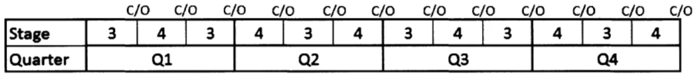
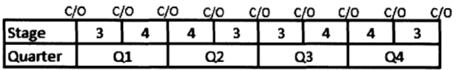
The production runs that are needed to for the two-module investment can be

found in Figure 5 and Figure 6 below:

C/o c/o C/o C/o C/o C/o C/o c/o C/o C/o c/o c/

Stage 1 2 1 2 1 21 1 2 1 2 1 2

Quarter Q1 Q2 Q3 Q4

Figure 5: Production schedule for first small module (base scenario)

C/o C/o c/o c/o C/o C/o C/o c/o c/o C/o c/o c/

Stage 3 4 3 4 3 4 3 4 3 4 3

I

4

Quarter Q1 Q2 Q3 Q4

Figure 6: Production schedule for second small module (base scenario)

This production run for the two-module investment would require that the first small module produce Stage 1 material, changeover, produce Stage 2 material, changeover, and then produce Stage 1 material all in Q1. Simultaneously, the second small module would need to produce Stage 3 material, changeover, produce Stage 4 material, changeover, and then produce Stage 4 material, all in Q1 as well. This essentially means that we can produce Stage 1, Stage 2, Stage 3 and Stage 4 material all in Q1 as compared to the one large module scenario where you could only produce Stage 1 and some Stage 2 material in Q1. As a result, in this production run format, the lead-time of the finished goods would be shorter and more adaptable should there be a spike in customer demand. However, the changeover frequency is comparatively higher.

In general, the objective of production is to match supply with demand and, in the real world, production scheduling is subject to many constraints such as demand forecast, set-up cost (time), equipment capacity, labor availability, etc. In our analysis, we simplify the production scheduling process by only considering the below constraints:

Demand constraint (D): Let D be the demand rate per year. In the base scenario, we assumed that the demand rate is certain and constant at 1 ton per week or 52 tons per year, and we need to produce exactly 52 tons of finished goods annually. So the

production quantity per year equals D.

Changeover lead time constraint: Each changeover takes 2 weeks. It takes two weeks to have the appropriate personnel to disinfect the module and prepare it for the next stage of production.

0

(22)

Changeover frequency constraint (CF): Let CF be the total number of changeovers per year, then the total available time that the equipment can actually be used to produce the product (AT) equals:

AT = 52 - CF*2 (1)

Once the above constraints are set, the production schedule can be determined, as shown in Appendix A.

Production Time for each batch (PT) is determined by the total production time and the number of batches running in each module. In other words, PT is the time in weeks that it takes to produce each batch. The number of batches equals the number of changeovers there are in each module. For example, if the changeover frequency is 4 times per year, the number of batches would be 4. Therefore, in one module, the PT equals:

52 - CF * 2

PT* = (2)

CF *The company assumes an integer value for PT.

The Average Production Quantity (APQ) per batch is determined by the total production quantity and the total number of batches per stage:

Total Production Quantity (Tons/Stage) (3)

Number of Batches/Stage

The equipment capacity (EC) measures the maximum tonnage of material that the equipment produces per unit of time. Integer values for the weekly production capacity were assumed to simplify calculations and were agreed upon with the sponsor company. The EC is therefore the average production quantity per batch, rounded up and divided

by the production time for each batch:

APQ

EC = roundup( PT (4)

As the production duration and production quantity is determined, the production schedule is thus settled.

(23)

4.2 Invertory

Once we set the demand rate, changeover lead time and changeover frequency, the production schedule is determined. Once the production schedule and demand rate

is known, we can easily calculate the average inventory.

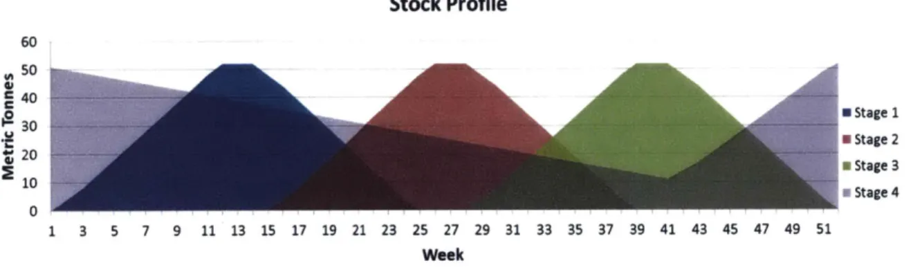
One Large Module Inventory: In the base scenario, we produce 52 tons of finished goods annually, with inventory levels varying between each production stage. In week 1, we assume that 52 tons of finished product (Stage 4) was being held in stock from the previous year's production and is slowly being shipped to the customer to meet demand. At the same time, in week 1, Stage 1 production begins and gradually produces stage 1 product until it reaches a maximum of 52 tons at the end of week 11 which is also equal to the total demand level that is needed at every production stage. Between week 12 and week 14, production halts and the changeover process begins, at which point quality personnel are tasked to disinfect the area and prepare it for the next stage of production (stage 2). As soon as stage 2 begins, stage 1 material begins to be consumed, producing stage 2 material, until it reaches a maximum of 52 tons in week 26. The same can be said about stage 3 and 4. Notice that as soon as stage 4 production begins in week 41, the stage 4 inventory level rises while the stage 3 inventory level drops (See Figure 7 for details). Stock Profile 60 450 S40 19 30 7Stage W20 Stage 3 10 Stage 4 0 1 3 5 7 9 11 13 15 17 19 21 23 25 27 29 31 33 35 37 39 41 43 45 47 49 51 Week

Figure 7: Stock profile of one module

According to the sponsor company, this large module scenario creates large batch sizes and little room for flexibility. In other words, if in Q1, the customer needed finished product, assuming there was no inventory of finished product in-house, the lead-time for the finished product would be 39 weeks starting from Raw Material. This calculation will be explained in detail in section 4.3.

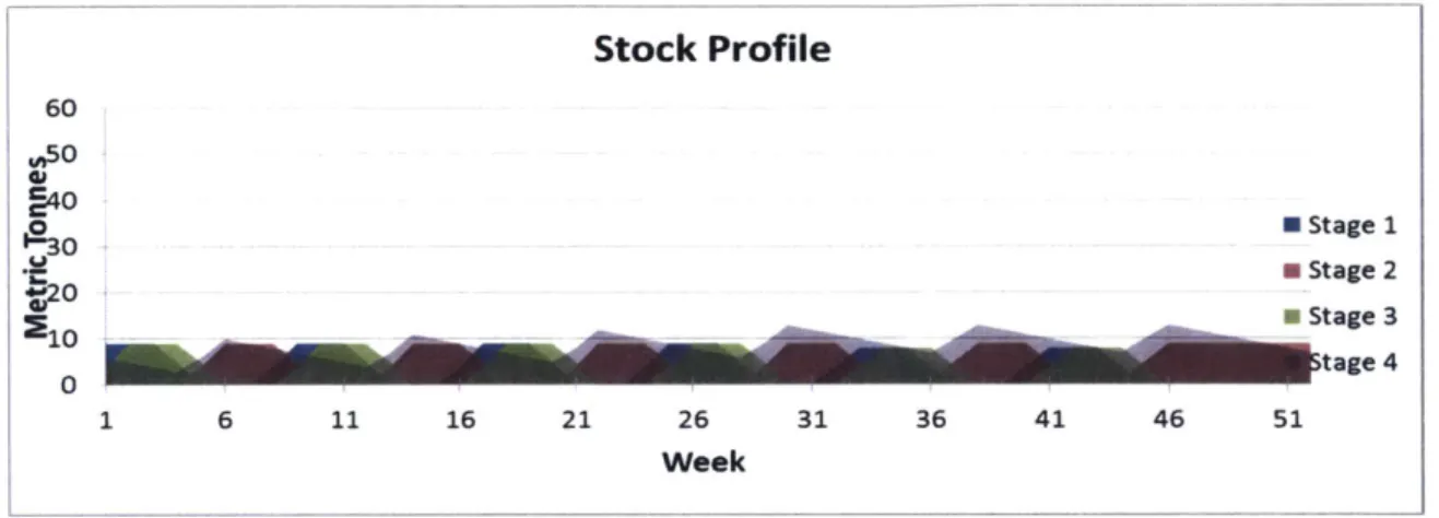
Two smaller modules Inventory: In the two smaller modules investment, the work in

process inventory is reduced. The output per module annually is the same at 52 tons. However, notice that the stage production runs are taking place more frequently. Stage

1, throughout the year, is being produced in batches of 8, 8, 8, 8, 10, 10 tons respectively,

(24)

Stock Profile 60 05 0 0 M Stage 1 -A20 ! Stage 2 W0 _{Stage 3} M0 0 __tage 4 1 6 11 16 21 26 31 36 41 46 51 Week

Figure 8: Stock profile for two smaller modules investment

4.3 Lead Time

Lead time is defined as the amount of time it takes to produce one unit of finished goods from raw material. The lead time (LT) equals the amount of time the previous stages take up until the current point in time plus the time spent on changeovers:

LT = (SG - 1) * PT + SG* 2 (5)

In the base scenario, with one-module investment, the lead time to start producing finished goods equals:

LT = (4 - 1) * 11+ 4 * 2 = 39 weeks (6)

With a two-module investment, the lead time equals:

LT = (4 - 1) * 2 + 4 * 2 = 14 weeks (7)

4.4 Changeovers

In the base scenario, the production process in the two-module investment requires a total of 6 changeovers in one quarter and, consequently, 24 changeovers in one year as compared to 4 changeovers in the one large module investment. The 24 changeovers is equivalent to:

24 changeovers x 2 weeks/changeover = 48 weeks required for changeover annually In the same manner, the 4 changeovers in the one large investment is equivalent to:

4 changeovers x 2 weeks/changeover = 8 weeks requiredfor changeover annually This is why it is important to incorporate the changeover cost into our model. With more frequent changeover, there is more wasted time during which the equipment does not produce any material. In order to achieve the same production output, more

(25)

production capacity is needed. We define equipment capacity as the maximum amount of products that can be produced during a certain period of time. The higher the capacity of equipment is, the larger the size of the equipment, and the higher the equipment capital investment. For simplicity, we assume that equipment cost is proportional to equipment capacity. In the one module investment, the maximum output is 5 tons per week and the equipment costs E30 million. In two modules, the maximum output is 4 tons per week for each equipment and thus 8 tons per week for both modules. The total equipment for both modules then costs E48 million. Production capacity is increased in exchange for the inventory reduction and increased flexibility.

In section 5 of this paper we look at different scenarios in which we adjust the production schedule to look at the impact on inventory level, production capacity and

NPV. For instance, we studied whether it would make sense to have 2 changeovers in one

quarter as opposed to 3 changeovers, and how that impacts the total cost of the investment as well as on other KPI's.

Changeover frequency also affects the utilization rate of production equipment. The higher the utilization rate, the higher the output that can be produced per module. However, the tradeoff is flexibility; the higher the utilization rate, the lower the excess capacity available to handle fluctuations in demand. The utilization rate is defined as:

Actual Annual Production Volume (8)

Production Utilization Rate =

Maximum Annual Production Capacity

For example, for the base scenario and for one module:

Actual Annual Production Volume = 52 tons *4 stages ()

stage year

5 tons (10)

Maximum Annual Production Capacity = 52 weeks * week

week

52*4 (11)

Production Utilization Rate = 52 80%

52

4.5 Free Cash Flows and Net Present Value

The cost breakdown spreadsheet that we had was linked to an Income Statement spreadsheet. We set it up this way in order for us to test how changes in any of the elements would impact the NPV.

(26)

Using the company's financial statements, we were able to estimate the revenues and ultimately calculate the free cash flows (FCF). Using the free cash flows, we were able to calculate the Net Present Value (NPV) of the investment decisions. Although this analysis is not enough to make an expensive investment decision, it gives us and the sponsor company a framework to work with and informs us as to whether an investment is or is not favorable. Furthermore, should the cost breakdown not be fully accurate, at the very least, it provides us with a technique to comparatively analyze the investments. The projected free cash flows are demonstrated in

Assumptions

Tax Rate _20%

Discount Rate 9%

Incremental Income Statement

Remenue

-COGS

= Gross Income

Periods:

-Operating Expenses

= Operating Income (EBITDA)

-Depreciation & Amortization

Depir.tcl

= Operating Income (EBIT)

-Income Tax

= Net Operating Profit After Taxes (NOPAT)

Adjustments

+ Depreciation (not a cash flow) -Net Capital Expenditures

Eqwl'mena

Module

-Net Working Capital Instment

+ Nei increase in Accounts Receivablc

+ Net increase in Inventory

- Net tncreo-si .o Acons

PaiyiNrr-Free Cash Flow

E E E -E 0 0.00 0.00 - 0.00 -E 0.00 E E E E E E E E 1 88.52 21.76 66.76 2.22 64.54 5.05 5.05 59.49 11.90 E f E f f E E E E 88.52 21.76 66.76 2.22 64.54 5.05 5 05 59.49 11.90 f f E E E E E E 88.52 21.76 6676 2.22 64.54 5.05 5 05 59.49 11.90 E E E E E E E 10 88.52 21.76 66.76 2.22 64.54 5.05 5 05 59.49 11.90 -E 0.00 E 47.59 f 47.59 E 47.59 E 47.59 Salvage Salvage E 5.05 E 5.05 E 5.05 E 5.05 E 58.00 E - E - E - E -E 46.00 S 1000 E 4.28 E - E - E - E -F 4 275 E E -f 62.28 E 52.64 E 52.64 E 52.64 E 52.64 NPV E 275.58 Figure 9: Assumptions Tax Rate Discount Rate

Incremental Income Statement

Resenue -COGS = Gross Income 9% Periods:| -Operating Expenses

= Operating Income (EBITDA)

-Depreciation & Amortization Operating Income (EBIT)

- Income Tax

= Net Operating Profit After Taxes (NOPAT)

Adjustments

+ Depreciation (not a cash flow)

- Net Capital Expenditures

Equipmet

Module

- Net Working Capital Inestment

4 Net lnc.rease.iu Ac; icutli, Reiereivdlt,

SNet Inc rease in inventory

Not ic!rese in Accouots Pay 707+

Free Cash Flow

0 -E0 -E0 0.00 0.00 0.00 0.00 E E E E E E 88.52 21.28 67.24 1.26 65.98 3.25 62.73 12.55 E E E E E E E 88.52 21.28 67.24 1.26 65.98 3.25 62.73 12.55 E E E E E E E E 3 88.52 21.28 67.24 1.26 65.98 3.25 62.73 12.55 E E E E E E E 10 88.52 21.28 67.24 1.26 65.98 3.25 62.73 12.55 -E 0.00 E 50.19 E 50.19 E 50.19 f 50.19 E 3.25 E 3.25 E 3.25 E 3.25 E 40.00 E - E - E - E -i 30 00 E 10 00 E 8.24 E - E - E - E -f 5 24 E E 48.24 E 53.44 E 53.44 E 53.44 ... E 53.44 NPV E 294.70 -A9

(27)

Assumptions

Tax Rate

Discount Rate

Incremental Income Statement

20% 9% Periods-: Revenue -COGS = Gross Income -Operating Expenses Operating Income (EBITDA)

-Depreciation & Amortization

Deprecidtiwn = Operating Income (EBIT)

-Income Tax

= Net Operating Profit After Taxes (NOPAT) Adjustments

+ Depreciation (not a cash flow)

-Net Capital Expenditures

Equi;),iw,)!

-Net Working Capital Investment

+ Nt !clow e ! A R w Free Cash Flow

E E E -E E -E -E 0.00 0.00 0.00 0.00 E E E E E E E 1 88.52 21.76 66.76 2.22 64.54 5.05 5 (15 59.49 11.90 E E E E E E E. E E 2 88.52 21.76 66.76 2.22 64.54 5.05 5 05 59.49 11.90 E E E E E E E E 3 88.52 21.76 66.76 2.22 64.54 5.05 5 05 59.49 11.90 E E E E E E E E E 10 88.52 21.76 66.76 2.22 64.54 5.05 5 05 59.49 11.90 -f 0.00 E 47.59 E 47.59 f 47.59 E 47.59 Salvage Salvage E 5.05 E 5.05 E 5.05 E 5.05 E 58.00 E - E - E - E -f 46 00 E 1 6 00 E 4.28 E - E - E - E -E 4 28 E - --E 62.28 E 52.64 E 52.64 E 52.64 E 52.64 NPV E 275.58

Figure 9: Free Cash Flow Analysis for the One Module Baseline Scenario

The FCF is calculated using the following formula:

FCF = NOPAT + Deprecitiaion - Net Capital Expenditures

- Net Working Capital Investment

(12)

As mentioned earlier in the paper, we calculated the FCF for the investment over

10 years with the assumption that the tax rate was 20% and the discount rate was 9%.

Here we assumed annuity but no perpetuity. This same FCF analysis was done for all 11 scenarios.

Next we calculated the NPV for the investments in our base scenarios as well as the additional scenarios we had proposed. This was important because not only did we want to identify whether this type of investment is profitable but also use NPV as a benchmark to compare the different scenarios. For instance, is there a big difference between the NPV, and how much flexibility do we have to make the first investment more attractive than the second and vice versa? This will be important for our scenario testing section of this paper.

4.6 Key Performance Indicators

We performed this comparative analysis by focusing on how different scenarios impacted key performance indicators. The KPI's that we thought would be most useful to the sponsor company are:

(28)

Net-present value (NPV): The NPV here would be crucial since it is important for key

stakeholders at the company to decide from the very start whether to proceed with an investment. The NPV is also important when comparing the different investments. It becomes a lot easier to recommend specifictypes of investments based on the NPV alone but should also be supported by other metrics.

Finished Goods Lead-time (L/T): Assuming a four-stage production process and no finished goods inventory available at the start of the year, the finished goods do not become readily available until the fourth quarter (Q4) when stage 3 is complete, changeover takes place and then Stage 4 is initiated. This means that it takes approximately 39 weeks to go from raw materials to finished goods. Should there be a sudden surge in demand, it would take approximately 39 weeks to provide the customer with the product assuming there is no finished goods inventory available in-house. Depending on the urgency of the matter, this could be manageable or it could be an operational bottleneck.

Machine Operating Time Rate (MOT): The machine operating time rate varies

significantly between the first and second investment. This rate is inversely correlated to the changeover frequency; as the changeover frequency increases, the MOT rate decreases. In the first investment we studied, there were four changeovers per year at a duration of two weeks per changeover. This implied that the production facility was utilized 84% of the entire year. Assuming there are no changeovers whatsoever, which is not likely, the MOT increases to 100%. It is important to understand that it is not uncommon to find low MOT rates in the pharmaceutical industry.

Equipment Capacity (EC): This measures the maximum production rate of equipment. In

the one-module case under the base scenario, the maximum output of one equipment is

5 tons per week. Maximum output is the maximum tonnage of material that the

equipment can produce per unit of time. This rate, multiplied by the amount of time the equipment is scheduled for production, determines the total production capacity.

Equipment Investment (El): Equipment investment takes up the majority of upfront

capital investment, and thus has the highest influence on the capital expenditure in our

NPV analysis. The higher the El is, the lower the NPV will be. El is proportional to the EC

of the equipment.

Allowable demand variation (DV): The maximum production quantity under the existing

production schedule equals the maximum output times the production time. So DV equals:

MO * PT (13)

DV =

D

Work in process Inventory (WIP): In the base scenario, the average work-in-process

inventory is 8.24 million for the one-module investment but is reduced to about E4.28

(29)

company has had an objective for the last couple of years to reduce inventory, so this is an important metric to pay attention to, but will also come at a cost.

Profitability Index (P1): The Profitability Index here is an important metric that will provide us with a better understanding as to whether the investment is able to generate earnings, as compared to the initial investment that was made. The profitability index equation is as follows:

NPV (14)

Profitability Index = ia Ivte

Initial Investment

4.7 Scenario Testing

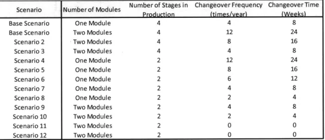
It is not enough to say that either of the investments is more attractive than the other solely based on the NPV. Therefore, it is important to experiment with the results, generate different scenarios to identify when any of the investments move from being less attractive to being more attractive and vice versa. In order to do this we have set up 12 different scenarios that vary the changeover frequency and consider both 4 stage production and 2 stage production. As mentioned earlier, we assumed demand to be constant at 52 tons a year. A summary of the scenario analysis that we have done can be

found in Figure 10 below:

Scenario Number of Modules Number of Stages in Changeover Frequency Changeover Time

Production (times/vear) (Weeks)

Base Scenario One Module 4 4 8

Base Scenario Two Modules 4 12 24

Scenario 2 Two Modules 4 8 16

Scenario 3 Two Modules 4 4 8

Scenario 4 One Module 2 12 24

Scenario 5 One Module 2 8 16

Scenario 12 Two Modules 2 0 0

Figure 10: Scenario Assumption S ummary

Changeover Frequency: We have varied changeover frequency which, as we have mentioned earlier, has a direct correlation to the equipment investment.

Number of production stages: We varied the number of production stages from 4 stages to 2 stages. The sponsor company advised that it is not likely to find a production facility with more than four stages or less than 2 stages. On the contrary, it might be possible to find a production facility with two stages that produces a different product. We varied the production stages and studied the impact on WIP and NPV. From the base scenario

(30)

to scenario 3, we looked at products that take 4 stages to produce. Scenario 4 to scenario 12 require only two stages and produce a different set of products.

4.7.1 Base Scenario

For the base scenarios, the product takes 4 stages to produce and changeover frequency is 4 times per year for one module 12 times per year for two modules. 4.7.2 Scenario 2 to 3

For these scenarios, all else remains the same as base scenario, except the changeover frequency. In scenario 2, the changeover frequency for two modules is 12 times a year. For scenario 3, the frequency drops to 8 times a year. Stage 1 and 2 are produced in the first module, and stage 3 and 4 are produced in in the second module in parallel. See Figure 11 and Figure 12 for details.

C/o C/o C/o C1 / '1 I

iStage 1 2 I s r sn1 2 - r d

Quarter

0 1 02 03 Q4

Figure 11: Production schedule for scenario 2 -first module

C/o c/ clC cO C O C 0 CI

Stage 3 4 4 3 3 4 4 3

0r

Quarter 1 1 I Q2 Q3 Q4

Figure 12: Production schedule for scenario 2 - second module

In scenario 3 we further reduce the changeover frequency to 4 times

Figure 13 and Figure 14 for the schedule layout.

c/o C/o c/o

a year. See

C/o

Stage 1 2 1 2

Quarter Q1 Q2 Q3 Q4

Figure 13: Production schedule for scenario 3 -first module

c/o C/o Co C/o

Istage 3 4 3 4

Quarter Q1 Q2 Q3 Q4

Figure 14: Production schedule for scenario 3 - second module

4.7.3 Scenario 4 to Scenario 12

From scenario 4 to 12, we assume another type of product that only takes 2 production stages. Scenarios 4 to 8 test how the KPI's will change for a one module investment.

(31)

In scenario 4, we set the changeover frequency to 12 times a year. For scenarios

5 to 8, we set the frequency at 8, 6, 4 and 2 times per year.

Scenarios 9 to 12 examine a two-module investment and we set the changeover frequency at 4, 2, and 0 times per year respectively. Note that scenario 11 is a special case in which each module can only produce one stage throughout the year, so the changeover frequency is reduced to zero. Scenario 12 uses double the capacity as compared to

scenario 11.

5. Data Analysis and Results

In the previous sections, we collected cost data (labor, material, overhead, and depreciation), estimated revenue, net capital expenditures and net working capital. The data are all inputs into the free cash flow and net present value analysis model. The aim of the model is to identify the net present value as well as all the KPIs we mentioned in section 4 in order to compare all the scenarios.

In this section, we present the results and insights we gained from the analysis and breakdown of the different scenarios discussed in the previous section.

5.1 Scenario Analysis

We tested 12 different scenarios and identified how these KPIs varied with different scenario settings: Net-present value (NPV), finished goods Lead-time (L/T), production Utilization Rate (UR), Equipment Capacity (EC), Equipment investment (EI), allowable Demand Variation (DV), Work-In-Process inventory (WIP), Profitability Index (PI) etc. The two key variables that we changed are changeover frequency (CF) and the number of stages (SG) in the production process.

(32)

4 Stages

One Module Two Modules

Base Base Scenario Scenario

Scenario Scenario 2 3

Changeover Frequency (CF) (times/year) 4 12 8 4

Number of Stages/module 4 2 2 2

ChangeoverTime (Weeks) 8 24 16 8

Number of batches/module 4 12 8 4

Total Production Time 44 28 36 44

AVG production quantity for each batch 52.0 8.7 13.0 [26.0

Production time for each batch (Week/batch) 11.0 2.3 4.5 11. 0

Equipment Capacity (Tons/week) 5 4 3 3

Maximum Annual Production Capacity (Tons) 260 208 156 t 156

Actual Annual Production Volume (Tons/year) 208 104 104 104

Production Utilization Rate (%) 80%

1

50% 67% 67%

Machine Operating Time Rate (%) 85%

1

54% 69% . 85%

Actual Production Volume (Tons) 52 52 52 52

Maximum Production Quantity (Tons) 55 56 54

I

66

Allowable Demand Fluctuation % 6% t 8% 4% L 27%

Inventory Investment (EM) 8.24 3.68 4.32 6.22

Lead Time (weeks) 39 14 20 41

Profitability Index (%) 610.9%

1

447.8% 571.4% 547.0%

Module Investment (EM) 10 10 10 10

Equipment Investment (EM) 30 48 36

1

36

Total Capital Investment (EM) 48.24 61.68 50.32 52.22

NPV 294.70 276.18 287.53 285.64

Analyzing tradeoffs between working capital and production capacity for multi-stage manufacturing processes

Signature redacted

redacted

Signature redacted_

11 201

Signature redactedThssSprio

7,

JUN 3 0

2016

LIBRARIES

ARCHIVES

Abstract

Biographical Notes

Acknowledgements

TABLE OF CONTENTS

LIST OF FIGURES

LIST OF TABLES

1. Introduction

2. Literature Review

-I

3. Data Collection

4. Methodology and Approach

I

Quarter

5. Data Analysis and Results

1

1

I

1

1