Benchmark Solutions For Transport In $d$-Dimensional Markov Binary Mixtures

(1)

HAL Id: cea-02434546

https://hal-cea.archives-ouvertes.fr/cea-02434546

Submitted on 10 Jan 2020

HAL is a multi-disciplinary open access

archive for the deposit and dissemination of

sci-entific research documents, whether they are

pub-lished or not. The documents may come from

teaching and research institutions in France or

abroad, or from public or private research centers.

L’archive ouverte pluridisciplinaire HAL, est

destinée au dépôt et à la diffusion de documents

scientifiques de niveau recherche, publiés ou non,

émanant des établissements d’enseignement et de

recherche français ou étrangers, des laboratoires

publics ou privés.

Markov Binary Mixtures

C. Larmier, F.-X. Hugot, F. Malvagi, A. Mazzolo, A. Zoia

To cite this version:

C. Larmier, F.-X. Hugot, F. Malvagi, A. Mazzolo, A. Zoia. Benchmark Solutions For Transport In

d-Dimensional Markov Binary Mixtures. M&C 2017 - International Conference on Mathematics and

Computational Methods Applied to Nuclear Science and Engineering, Apr 2017, Jeju, South Korea.

�cea-02434546�

(2)

Benchmark solutions for transport in d-dimensional Markov binary mixtures

Coline Larmier,∗_{François-Xavier Hugot,}∗_{Fausto Malvagi,}∗_{Alain Mazzolo,}∗_{Andrea Zoia,}∗

∗_{Den-Service d’études des réacteurs et de mathématiques appliquées (SERMA), CEA, Université Paris-Saclay, F-91191,}

Gif-sur-Yvette, France andrea.zoia@cea.fr

Abstract - Particle transport in random media obeying a given mixing statistics is key in several applications in

nuclear reactor physics and more generally in diffusion phenomena emerging in physics and life sciences. Exact

solutions for the ensemble-averaged physical observables are hardly available, and several effective models have been thus developed, providing a compromise between the accurate treatment of the disorder-induced spatial correlations and the computational time. In order to validate these models, it is mandatory to resort to reference solutions. We extend the pioneering work by Adams, Larsen and Pomraning [1] (recently revisited by Brantley [2]) by considering a series of benchmark configurations for mono-energetic and isotropic transport through Markov binary mixtures in dimension d. The stochastic media are generated by resorting to Poisson

random tessellations in1d slab, 2d extruded, and full 3d geometry. For each realization, particle transport

is performed by resorting to Monte Carlo simulation. The distributions of the transmission and reflection

coefficients on the free surfaces of the geometry are subsequently estimated, and the average values over the

ensemble of realizations are computed. Reference solutions for the benchmark have never been provided before for two- and three-dimensional Poisson tessellations, and the results presented in this paper might thus be useful in order to validate fast but approximated models for particle transport in Markov stochastic media, such as the celebrated Chord Length Sampling algorithm.

I. INTRODUCTION

Linear transport through heterogeneous and disordered media emerges in several applications in nuclear science and engineering. Examples are widespread and concern for

in-stance neutron diffusion in pebble-bed reactors or randomly

mixed immiscible materials [3, 4], and inertial confinement fu-sion [5]. The key goal of particle transport theory in stochastic media consists in deriving a formalism for the description of the ensemble-averaged angular particle flux hϕ(r, ω)i, where ϕ(r, ω) solves the linear (single-speed) Boltzmann equation

ω · ∇ϕ + Σ(r)ϕ =Z Σs(ω0→ω, r)ϕ(r, ω0)dω0+ S, (1)

r and ω denoting the position and direction variables,

respec-tively,Σ(r) being the total cross section, Σs(ω0→ω, r) the

dif-ferential scattering cross section, and S = S (r, ω) the source

term. For isotropic scattering, the differential scattering cross

section simplifies toΣs(ω0 → ω, r) = Σs(r)/Ωd, whereΩd

is the surface area of the unit sphere in dimension d. The stochastic nature of particle transport stems from the materials composing the traversed medium being randomly distributed

according to some statistical law. Hence, the quantitiesΣ(r),

Σs(ω0→ω, r) and S (r, ω) are in principle random variables.

A widely adopted model of random media is the so-called bi-nary stochastic mixing, where only two immiscible materials (say α and β) are present [3]. Then, by averaging Eq. (1) over realizations having material α at r, we obtain the following

equation for hϕα(r, ω)i

[ω · ∇+ Σα] pαhϕαi= pα_ΩΣ_ds,α Rhϕα(r, ω0)idω0+ pαSα

+pβ,αhϕβ,αi − pα,βhϕα,βi (2)

where pi(r) is the probability of finding the material of index

iat position r. Here pi, j = pi, j(r, ω) denotes the probability

per unit length of crossing the interface from material i to material j for a particle located at r and travelling in direction

ω, and hϕi, ji denoting the angular flux averaged over those

realizations where there is a transition from material i to mate-rial j for a particle located at r and travelling in direction ω.

The cross sectionsΣαandΣs,αare those of material α. The

equation for hϕβ(r, ω)i is immediately obtained from Eq. (2)

by permuting the indexes α and β.

The set of equations in Eq. (2) can be shown to form an infinite hierarchy [3, 4]. Generally speaking, it is therefore nec-essary to introduce a closure formula, depending on the under-lying mixing statistics. The celebrated Levermore-Pomraning

model assumes for instance hϕα,βi= hϕαi for homogeneous

Markov mixing statistics [3], which is defined by

pi, j(r, ω)= _Λpi

i(ω)

, (3)

depending on the starting position alone, whereΛi(ω) is the

mean chord length for trajectories crossing material i in direc-tion ω. Several generalisadirec-tions of this model have been later proposed, including higher-order closure schemes [3]. In par-allel, Monte Carlo algorithms such as the Chord Length Sam-pling have been conceived in order to address the Levermore-Pomraning model, and have been further extended so as to

include partial memory effects due to correlations for particles

crossing back and forth the same materials [5]. Their com-mon feature is that they allow a simpler, albeit approximate, treatment of transport in stochastic mixtures, which might be convenient in practical applications.

In order to assess the accuracy of the various approximate models it is therefore mandatory to compute reference solu-tions for the exact Eqs. (2). Such solusolu-tions can be obtained in the following way: first, a realization of the medium is

(3)

sampled from the underlying mixing statistics; then, the linear transport equations corresponding to this realization are solved by either deterministic or Monte Carlo methods, and the phys-ical observables of interest are determined; this procedure is

repeated many times so as to create a sufficiently large

collec-tion of realizacollec-tions, and ensemble averages are finally taken for the physical observables. For this purpose, a number of benchmark problems for Markov mixing have been proposed in the literature so far [1, 4, 2], with focus exclusively on 1d geometries, either of the rod or slab type.

In this work we will revisit the classical benchmark prob-lem proposed by Adams, Larsen and Pomraning for transport in stochastic media [1]. We will present reference solutions obtained by Monte Carlo particle transport simulation through 1d slab, 2d extruded and 3d tessellations of a finite-size box with Markov mixing. We will compute the particle flux hϕi,

the transmission coefficient hTi and the reflection coefficient

hRi by taking ensemble averages over the realizations; the dispersion of the physical observables around their average values will be assessed by evaluating their full distributions. Benchmark solutions for transport in 2d extruded and 3d tes-sellations have never been addressed before.

II. BENCHMARK SPECIFICATIONS

The benchmark specifications for our work are essen-tially taken from those originally proposed in [1, 4], and later extended in [2]. We consider single-speed linear par-ticle transport through a stochastic binary medium with ho-mogeneous Markov mixing. The medium is non-multiplying, with isotropic scattering. The geometry consists of a cubic

box of side L = 10, with reflective boundary conditions on

all sides of the box except two opposite faces (say those per-pendicular to the x axis), where leakage boundary conditions are imposed: particles that leave the domain through these faces can not re-enter. Lengths are expressed in arbitrary units.

In [1] and [4], system sizes L = 0.1 and L = 1 were also

considered, but in this work we will focus on the case L= 10,

which leads to more physically relevant configurations. Two kinds of non-stochastic sources have been considered in [2], namely, an imposed normalized incident angular flux on the

leakage surface at x = 0 (with zero interior sources), or a

distributed homogeneous and isotropic normalized interior source (with zero incident angular flux on the leakage sur-faces). The benchmark configurations pertaining to the former kind of source have been conventionally called suite I, whereas those pertaining to the latter have been called suite II [2]. In this work, we will present the simulation results for suite I, and we refer the reader to a companion work [?] for those of

suiteII. The material properties for the Markov mixing are

entirely defined by assigning the average chord length for each

material i= α, β, namely Λi, which in turn allows deriving

the homogeneous probability pi of finding material i at an

arbitrary location within the box, namely, pi= Λi/(Λi+ Λj).

The material probability pidefines the volume fraction for

ma-terial i. The cross sections for each mama-terial will be denoted as

customaryΣifor the total cross section andΣs,ifor the

scatter-ing cross section. The average number of particles survivscatter-ing

a collision in material i will be denoted by ci = Σs,i/Σi ≤ 1.

The physical parameters for the benchmark configurations are recalled in Tabs. I and II: three cases (numbered 1, 2 and 3) are considered, each containing three sub-cases (noted a, b and c). The case numbers correspond to varying the materials,

whereas the sub-cases represents varying ratios of cifor each

material.

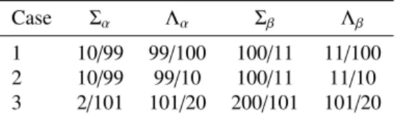
Case Σα Λα Σβ Λβ

1 10/99 99/100 100/11 11/100

2 10/99 99/10 100/11 11/10

3 2/101 101/20 200/101 101/20

TABLE I. Material parameters for the three cases of the bench-mark configurations.

Sub-case a b c

cα 0 1 0.9

cβ 1 0 0.9

TABLE II. Material parameters for the three sub-cases of the benchmark configurations.

The physical observables of interest for the proposed benchmark will be the ensemble-averaged outgoing parti-cle currents hJi on the two surfaces with leakage boundary conditions, and the ensemble-averaged scalar particle flux

hϕ(x)i = hR R R ϕ(r, ω)dωdydzi along 0 ≤ x ≤ L. For

the suite I configurations, the outgoing particle current on the side opposite to the imposed current source will

repre-sent the ensemble-averaged transmission coefficient, namely,

hT i= hJx=Li, whereas the outgoing particle current on the side

of the current source will represent the ensemble-averaged

re-flection coefficient, namely, hRi = hJx=0i.

III. POISSON GEOMETRIES

Poisson geometries form a prototype process of isotropic stochastic tessellations: a portion of a d-dimensional space is partitioned by randomly generated (d − 1)-dimensional hyper-planes drawn from an underlying Poisson process [6]. An explicit construction amenable to Monte Carlo realiza-tions for two-dimensional homogeneous and isotropic Pois-son geometries of finite size has been established in [7]. A generalization of this algorithm to three-dimensional (and in principle d-dimensional) domains has recently been pro-posed [8], based on a spatial tessellation of the d-hypersphere of radius R centered at the origin by a random number m of (d − 1)-hyperplanes with random orientation and

posi-tion. The number m of (d − 1)-hyperplanes is sampled

from a Poisson distribution with parameter ρRAd(1)/Vd−1(1).

Here Ad(1) = 2πd/2/Γ(d/2) denotes the surface of the

d-dimensional unit sphere (Γ(a) being the Gamma function),

Vd(1) = πd/2/Γ(1 + d/2) denotes the volume of the

d-dimensional unit sphere, and ρ is the arbitrary density of the tessellation, carrying the units of an inverse length.

(4)

Case 1, d= 1

Case 1, d= 2

Case 1, d= 3

Fig. 1. Examples of realizations of Poisson geometries cor-responding to the benchmark specifications for the 1d slab tessellations (top), 2d extruded tessellations (middle) and 3d tessellations (bottom), before (left) and after (right) attributing the material label. Red denotes label α and blue denotes label

β. For case 1, pα= 0.9.

in [1], based on the Poisson process on the line. For the 2d ex-truded tessellations, we begin by creating an isotropic Poisson tessellation of a square of side L, according to the algorithm detailed in [9]. By construction, the polygons defined by the intersection of random lines drawn according to this method are convex. Once the square has been tessellated, the full geometrical description for the cube is simply achieved by extruding the random polyhedra (which lie on the x − y plane) along the orthogonal z axis (see Fig. 1).

Let us now focus on 3d tessellations [10]. We denote by R the radius of the sphere circumscribed to the cube, and suppose that the cube is centered in the origin O. We start again by sampling a random number of points m from a Poisson

distribu-tion of parameter 4ρR, where we have used A3(1)/V2(1)= 4.

Then we generate the planes that will cut the cube. We choose a radius r uniformly in the interval [0, R] and then sample two

additional parameters, namely, ξ1and ξ2, from two

indepen-dent uniform distributions in the interval [0, 1]. A unit vector

n= (n1, n2, n3)Tis generated, with components n1= 1 − 2ξ1,

n2 = q 1 − n2 1cos (2πξ2), and n3 = q 1 − n2 1sin (2πξ2). Let

now M be the point such that OM= rn. The random plane

will finally obey n1x+ n2y+ n3z= r, passing trough M and

having normal vector n. The procedure is iterated until m random planes have been generated. The polyhedra defined by the intersection of such random planes are convex (see Fig. 1). Poisson geometries satisfy a Markov property: for do-mains of infinite size, arbitrary drawn lines will be cut by the (d − 1)-surfaces of the d-polyhedra into segments whose

lengths ` are exponentially distributed, i.e., P(`)= ρe−ρ`, with

average h`i = R `P(`)d` = 1/ρ [6]. The quantity Λ = 1/ρ

intuitively defines the correlation length of the Poisson geom-etry, i.e, the typical linear size of a volume composing the random tessellation.

Binary Markov mixtures required for the benchmark spec-ifications are obtained as follows: first, a d-dimensional Pois-son tessellation is constructed as described above. Then, each polyhedron of the geometry is assigned a material composition by formally attributing a distinct ‘label’ (also called ‘color’),

say ‘α’ or ‘β’, with associated complementary probabilities pα

and pβ= 1 − pα. Adjacent polyhedra sharing the same label

are finally merged. This gives rise to (generally) non-convex α and β clusters, each composed of a random number of convex polyhedra. The statistical features of Poisson binary mixtures, including percolation probabilities and exponents, have been previously addressed in [9] for 2d geometries and in [10] for 3d geometries. It can be shown that the average chord length

Λαthrough clusters with composition α is related to the

corre-lation lengthΛ of the geometry via Λ = (1− pα)Λα, and forΛβ

we similarly haveΛ = pαΛβ. This yields 1/Λα+ 1/Λβ = 1/Λ,

and we recover

pα = Λ

Λβ =

Λα

Λα+ Λβ. (4)

Thus, based on the formulas above, and using ρ= 1/Λ, the

parameters of the colored Poisson geometries corresponding to the benchmark specifications provided in Tab. I are easily derived. For the purpose of illustration, examples of realiza-tions of Poisson geometries for the case 1 of the benchmark are displayed in Fig. 1 for the 1d slab tessellations, the 2d extruded tessellations and the 3d tessellations.

IV. SIMULATION PARAMETERS

The reference solutions for the ensemble-averaged scalar particle flux hϕ(x)i and the currents hRi and hT i have been computed as follows. For each benchmark case and sub-case, a large number M of geometries has been generated, and the material properties have been attributed to each volume as described above. Then, for each realization k of the ensemble, linear particle transport has been simulated by resorting to

the production Monte Carlo code Tripoli-4 R_{, developed at}

CEA [11]. The number of simulated particle histories per

configuration is 106. For a given physical observable O, the

benchmark solution is obtained as the ensemble average

hOi= 1 M M X k=1 O_k (5)

where Okis the Monte Carlo estimate for the observable O

obtained for the k-th realization. Depending on the correla-tion lengths and on the volumetric fraccorrela-tions, the physical ob-servables might display a larger or smaller dispersion around

(5)

their average values. For 1d slab tessellations, we have taken

M = 104; for the 2d extruded tessellations, we have taken

M = 4 × 103_{; finally, for the 3d tessellations we have taken}

M = 103. As a general remark, increasing the dimension

implies an increasing computational burden (each realization takes longer both for generation and for Monte Carlo trans-port), but also a better statistical mixing (a single realization is more representative of the average behaviour). For reference, we have also computed transport results in configurations obeying the atomic mix approximation [3]: the findings corre-sponding to Poisson tessellations will be contrasted to those coming from the atomic mix model.

1. Computational time

For the simulations discussed here we have largely ben-efited from a feature that has been recently implemented in

the code Tripoli-4 R_{, namely the possibility of reading}

pre-computed connectivity maps for the volumes composing the geometry. During the generation of the Poisson tessellations, care has been taken so as to store the indexes of the neighbour-ing volumes for each realization, which means that durneighbour-ing the geometrical tracking a particle will have to find the following crossed volume in a list that might be considerably smaller than the total number of random volumes composing the box (depending on the features of the random geometry). To pro-vide an example, a typical realization of a 3d geometry for

case 1 will be composed of ∼ 105_{volumes, whereas the}

typi-cal number of neighbours for each volume will of the order of ∼ 10. When fed to the transport code, such connectivity maps allow thus for considerable speed-ups for the most fragmented geometries, up to one hundred.

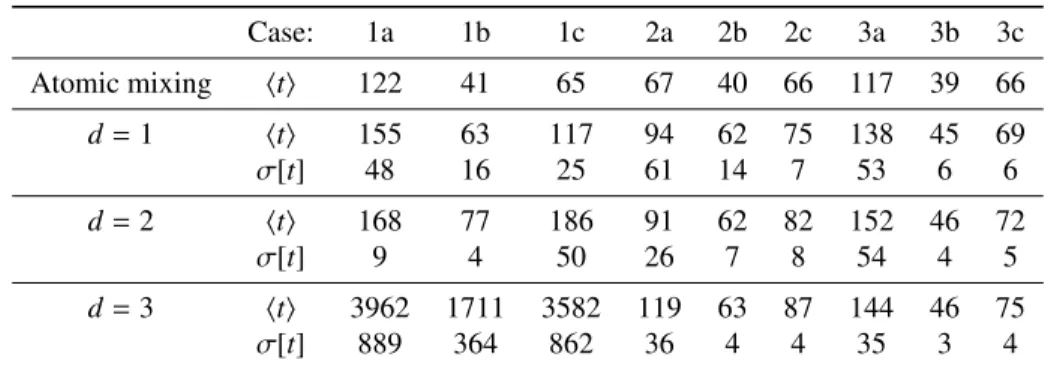
Transport calculations have been run on a cluster based at CEA, with Xeon E5-2680 V2 2.8 GHz processors. An overview of the average computer time hti for each benchmark configuration is provided in Tab. III. Dispersions σ[t] are also given. While an increasing trend for hti as a function of

dimension is clearly apparent, subtle effects due to correlation

lengths and volume fractions for the material compositions come also into play, and strongly influence the average com-puter time. For some configurations, the dispersion σ[t] may become very large, and even be comparable to the average hti. Atomic mixing simulations are based on a single homogenized realization, and the dispersion is thus trivially zero.

V. ANALYSIS OF MONTE CARLO SIMULATION RE-SULTS

1. Transmission, reflection and integral flux

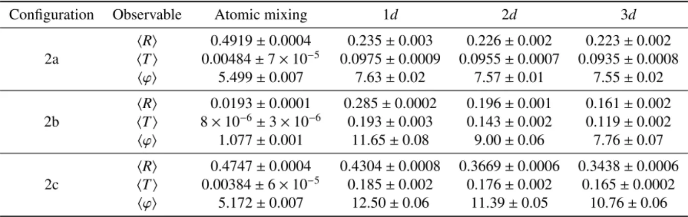
The simulation results for the ensemble-averaged

trans-mission coefficient hTi, the reflection coefficient hRi and the

integral flux hϕi= hR R ϕ(r, ω)dωdri are provided in Tabs. IV

to VI for all the benchmark configurations of suite I. Atomic mix results have been also given for reference. For each Monte Carlo transport simulation, the error on the estimated observ-able was significantly lower than 1%.

The computed values for the 1d slab configurations and the atomic mix approximation are in excellent agreement

(typ-ically to two or three digits) with those previously reported in [1, 2, 4], and allow concluding that our choice for the bench-mark specifications is coherent. For all examined cases, the atomic mix approximation generally yields poor results as compared with the benchmark solutions, and in some cases the discrepancy can add up to several orders of magnitude. In addition, the atomic mix solutions for several cases are strictly identical, since the ensemble-averaged total and scat-tering cross sections are identical by design. Concerning the

benchmark solutions in dimension d= 1, 2 and 3, the impact

of dimension on the transmission and reflection coefficient

is stronger between d = 1 and d = 2 than between d = 2

and d = 3, as expected on physical grounds, and has a large

variability between cases. The reflection coefficient hRi in

d= 1 is always larger than those in d = 2, 3. The transmission

coefficient hTi is also generally larger, apart from cases 1a, 1c,

and 3a, where it is smaller.

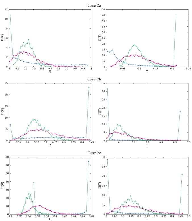
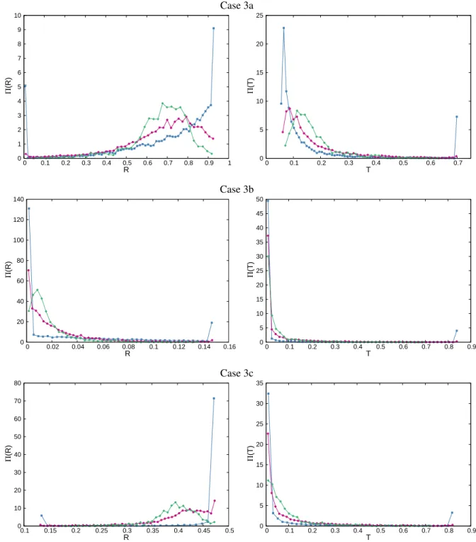
2. Distributions of transmission and reflection coefficients

In order to better assess the variability of the

transmis-sion and reflection coefficients around their average values,

we have also computed their full distributions based on the available realizations in the generated ensembles. The result-ing normalized histograms are illustrated in Figs. 2 to 4. As a general consideration, the dispersion of the observables de-creases with increasing dimension: the mixing is increasingly

efficient and the distribution is more peaked around the

aver-age, which is expected on physical grounds. However, even

for d = 3 it is apparent that several configurations display

highly non-symmetrical shapes, and possible cut-offs due to

finite-size effects. Especially in d = 1, bi-modality may also

arise for cases 2 and 3, which is due to the aforementioned

effect of random geometries being entirely filled with either

material α or β: the peaks observed in the distributions corre-spond to the values of the transmission or reflection coefficient associated to a fully red or fully blue realization. (The data sets of the distributions are available from the authors upon request.) For the 1d slab tessellations, the variances of the

transmission and reflection coefficient have been numerically

computed in [1]: the values obtained in our simulations are in excellent agreement with those previously reported.

VI. CONCLUSIONS

The key goal of this work was to compute reference so-lutions for linear transport in stochastic geometries. In order to establish a proper and easily reproducible framework, we have built our specifications upon the benchmark originally proposed by Adams, Larsen and Pomraning, and recently re-visited by Brantley. We have thus considered a box of fixed side, with two free surfaces on opposite sides, and reflecting boundary conditions everywhere else. As a prototype exam-ple of stochastic media, we have adopted Markov geometries with binary mixing: such geometries have been numerically implemented by resorting to the algorithm for colored Poisson geometries.

Three kinds of Poisson tessellations of the box have been tested: 1d slab tessellations, 2d extruded tessellations, and full

(6)

Case: 1a 1b 1c 2a 2b 2c 3a 3b 3c

Atomic mixing hti 122 41 65 67 40 66 117 39 66

d= 1 hti 155 63 117 94 62 75 138 45 69 σ[t] 48 16 25 61 14 7 53 6 6 d= 2 hti 168 77 186 91 62 82 152 46 72 σ[t] 9 4 50 26 7 8 54 4 5 d= 3 hti 3962 1711 3582 119 63 87 144 46 75 σ[t] 889 364 862 36 4 4 35 3 4

TABLE III. Simulation times t for the benchmark configurations, expressed in seconds. The cases of suite I.

3d tessellations. To the best of our knowledge, benchmark solutions for 2d and 3d tessellations with Markov mixing have never been studied before. Material compositions and correlation lengths, as well as source and boundary conditions, have been assigned based on the benchmark specifications. A large number of random geometries and material compositions have been realized. For each realization, mono-energetic linear transport with isotropic scattering and absorption has been

simulated by Monte Carlo method. The code Tripoli-4 R

developed at CEA has been used for this purpose.

The physical observables that have been examined in

this work are the reflection and transmission coefficients, and

the scalar particle flux, averaged over the ensemble of avail-able realizations. The full distributions of the reflection and

transmission coefficients have been also examined, in order

to evaluate the impact of correlation lengths and volumetric fractions on the dispersion of these observables around their average values.

VII. ACKNOWLEDGMENTS

The authors wish to thank Électricité de France (EDF) for partial financial support.

REFERENCES

1. M. ADAMS, E. LARSEN, and G. POMRANING, “Benchmark results for particle transport in a binary Markov statistical medium,” Journal of Quantitative Spec-troscopy and Radiation Transfer, 42, 253–266 (1989). 2. P. BRANTLEY, “A benchmark comparison of Monte

Carlo particle transport algorithms for binary stochas-tic mixtures,” Journal of Quantitative Spectroscopy and Radiation Transfer, 112, 599–618 (2011).

3. G. POMRANING, Linear kinetic theory and particle transport in stochastic mixtures, World Scientific Pub-lishing, River Edge, NJ, USA (1991).

4. O. ZUCHUAT, R. SANCHEZ, I. ZMIJAREVIC, and F. MALVAGI, “Transport in renewal statistical media: benchmarking and comparison with models,” Journal of Quantitative Spectroscopy and Radiation Transfer, 51, 689–722 (1994).

5. G. ZIMMERMAN and M. ADAMS, “Algorithms for Monte Carlo particle transport in binary statistical

mix-tures,” Transactions of the American Nuclear Society, 66, 287 (1991).

6. L. SANTALÓ, Integral geometry and geometric probabil-ity, Addison-Wesley, Reading, MA, USA (1976). 7. P. SWITZER, “Random set process in the plane with

Markov property,” Annals of Mathematical Statistics, 36, 1859–1863 (1965).

8. A. AMBOS and G. MIKHAILOV, “Statistical simulation of an exponentially correlated many-dimensional random field,” Russian Journal of Numerical Analysis and Mathe-matical Modelling, 26, 263–273 (2011).

9. T. LEPAGE, L. DELABY, F. MALVAGI, and A. MAZ-ZOLO, “Monte Carlo simulation of fully Markovian stochastic geometries,” Progress in Nuclear Science and Technology, 2, 743–748 (2011).

10. C. LARMIER, E. DUMONTEIL, F. MALVAGI, A. MAZ-ZOLO, and A. ZOIA, “Finite-size effects and percolation properties of Poisson geometries,” Physical Review E, 94, 012130 (2016).

11. E. BRUN, F. DAMIAN, C. DIOP, E. DUMONTEIL, F.-X. HUGOT, C. JOUANNE, Y.-K. LEE, F. MALVAGI, A. MAZZOLO, O. PETIT, J.-C. TRAMA, T. VISON-NEAU, and A. ZOIA, “TRIPOLI-4, CEA, EDF and AREVA reference Monte Carlo code,” Annals of Nuclear Energy, 82, 151–160 (2015).

(7)

Configuration Observable Atomic mixing 1d 2d 3d hRi 0.4919 ± 0.0004 0.435 ± 0.002 0.4031 ± 0.0006 0.4065 ± 0.0004 1a hT i 0.00484 ± 7 × 10−5 0.0147 ± 0.0002 0.0173 ± 0.0001 0.0162 ± 0.0001 hϕi 5.499 ± 0.007 6.09 ± 0.01 6.356 ± 0.008 6.318 ± 0.008 hRi 0.0193 ± 0.0001 0.0841 ± 0.0007 0.0453 ± 0.0002 0.0376 ± 0.0002 1b hT i 8 × 10−6_{± 3 × 10}−6 _{0.0017 ± 0.0001} _{0.00108 ± 3 × 10}−5 _{0.00085 ± 3 × 10}−5 hϕi 1.077 ± 0.001 2.89 ± 0.02 2.165 ± 0.005 1.920 ± 0.003 hRi 0.4747 ± 0.0004 0.4743 ± 0.0004 0.4059 ± 0.0004 0.4036 ± 0.0004 1c hT i 0.00384 ± 6 × 10−5 _{0.0159 ± 0.0003} _{0.0179 ± 0.0001} _{0.0164 ± 0.0001} hϕi 5.172 ± 0.0007 6.95 ± 0.03 6.52 ± 0.01 6.296 ± 0.0008

TABLE IV. Ensemble-averaged observables for the benchmark configurations: suite I - case 1.

Configuration Observable Atomic mixing 1d 2d 3d

hRi 0.4919 ± 0.0004 0.235 ± 0.003 0.226 ± 0.002 0.223 ± 0.002 2a hT i 0.00484 ± 7 × 10−5 0.0975 ± 0.0009 0.0955 ± 0.0007 0.0935 ± 0.0008 hϕi 5.499 ± 0.007 7.63 ± 0.02 7.57 ± 0.01 7.55 ± 0.02 hRi 0.0193 ± 0.0001 0.285 ± 0.0002 0.196 ± 0.001 0.161 ± 0.002 2b hT i 8 × 10−6_{± 3 × 10}−6 _{0.193 ± 0.003} _{0.143 ± 0.002} _{0.119 ± 0.002} hϕi 1.077 ± 0.001 11.65 ± 0.08 9.00 ± 0.06 7.76 ± 0.07 hRi 0.4747 ± 0.0004 0.4304 ± 0.0008 0.3669 ± 0.0006 0.3438 ± 0.0006 2c hT i 0.00384 ± 6 × 10−5 _{0.185 ± 0.002} _{0.176 ± 0.002} _{0.165 ± 0.0002} hϕi 5.172 ± 0.007 12.50 ± 0.06 11.39 ± 0.05 10.76 ± 0.06

TABLE V. Ensemble-averaged observables for the benchmark configurations: suite I - case 2.

Configuration Observable Atomic mixing 1d 2d 3d

hRi 0.7820 ± 0.0004 0.693 ± 0.003 0.672 ± 0.003 0.670 ± 0.004 3a hT i 0.0667 ± 0.0003 0.161 ± 0.002 0.170 ± 0.002 0.169 ± 0.003 hϕi 14.83 ± 0.02 16.35 ± 0.05 16.46 ± 0.05 16.35 ± 0.08 hRi 0.00202 ± 4 × 10−5 _{0.0349 ± 0.0004} _{0.0221 ± 0.0004} _{0.0167 ± 0.0006} 3b hT i 9 × 10−6_{± 3 × 10}−6 _{0.0740 ± 0.002} _{0.061 ± 0.002} _{0.045 ± 0.003} hϕi 1.004 ± 0.001 5.01 ± 0.06 4.08 ± 0.06 3.49 ± 0.08 hRi 0.4747 ± 0.0004 0.443 ± 0.001 0.406 ± 0.001 0.395 ± 0.001 3c hT i 0.00384 ± 6 × 10−5 _{0.101 ± 0.002} _{0.098 ± 0.002} _{0.085 ± 0.003} hϕi 5.172 ± 0.007 8.80 ± 0.07 8.34 ± 0.07 7.9 ± 0.1

(8)

Case 1a 0 10 20 30 40 50 60 70 0 0.1 0.2 0.3 0.4 0.5 0.6 0.7 0.8 0.9 Π (R) R 0 50 100 150 200 250 300 350 400 450 500 0 0.01 0.02 0.03 0.04 0.05 Π (T) T Case 1b 0 50 100 150 200 250 0 0.05 0.1 0.15 0.2 Π (R) R 0 500 1000 1500 2000 2500 3000 0 0.002 0.004 0.006 0.008 0.01 Π (T) T Case 1c 0 50 100 150 200 250 300 350 0.36 0.38 0.4 0.42 0.44 0.46 0.48 Π (R) R 0 50 100 150 200 250 300 350 0 0.01 0.02 0.03 0.04 0.05 0.06 Π (T) T

Fig. 2. Left column: normalized distributionsΠ(R) of the reflection coefficients R; right column: normalized distributions Π(T)

of the transmission coefficients T. Suite I configurations, case 1. Blue squares represent the 1d slab tessellations, red circles the

(9)

Case 2a 0 2 4 6 8 10 12 0 0.1 0.2 0.3 0.4 0.5 0.6 0.7 0.8 0.9 1 Π (R) R 0 5 10 15 20 25 30 35 40 45 50 0 0.05 0.1 0.15 0.2 0.25 Π (T) T Case 2b 0 5 10 15 20 25 0 0.05 0.1 0.15 0.2 0.25 0.3 0.35 0.4 0.45 Π (R) R 0 5 10 15 20 25 30 35 0 0.1 0.2 0.3 0.4 0.5 0.6 Π (T) T Case 2c 0 20 40 60 80 100 120 140 0.3 0.32 0.34 0.36 0.38 0.4 0.42 0.44 0.46 0.48 Π (R) R 0 5 10 15 20 25 30 0 0.05 0.1 0.15 0.2 0.25 0.3 0.35 0.4 0.45 0.5 Π (T) T

(10)

Case 3a 0 1 2 3 4 5 6 7 8 9 10 0 0.1 0.2 0.3 0.4 0.5 0.6 0.7 0.8 0.9 1 Π (R) R 0 5 10 15 20 25 0 0.1 0.2 0.3 0.4 0.5 0.6 0.7 Π (T) T Case 3b 0 20 40 60 80 100 120 140 0 0.02 0.04 0.06 0.08 0.1 0.12 0.14 0.16 Π (R) R 0 5 10 15 20 25 30 35 40 45 50 0 0.1 0.2 0.3 0.4 0.5 0.6 0.7 0.8 0.9 Π (T) T Case 3c 0 10 20 30 40 50 60 70 80 0.1 0.15 0.2 0.25 0.3 0.35 0.4 0.45 0.5 Π (R) R 0 5 10 15 20 25 30 35 0 0.1 0.2 0.3 0.4 0.5 0.6 0.7 0.8 0.9 Π (T) T