HAL Id: inria-00070426
https://hal.inria.fr/inria-00070426
Submitted on 19 May 2006
HAL is a multi-disciplinary open access
archive for the deposit and dissemination of
sci-entific research documents, whether they are
pub-L’archive ouverte pluridisciplinaire HAL, est
destinée au dépôt et à la diffusion de documents
scientifiques de niveau recherche, publiés ou non,
network study
Céline Fouard, Grégoire Malandain, Steffen Prohaska, Malte Westerhoff
To cite this version:
Céline Fouard, Grégoire Malandain, Steffen Prohaska, Malte Westerhoff. Blockwise processing applied
to brain micro-vascular network study. [Research Report] RR-5581, INRIA. 2005, pp.27.
�inria-00070426�
ISRN INRIA/RR--5581--FR+ENG
a p p o r t
d e r e c h e r c h e
Thème BIO
Blockwise processing applied to brain
micro-vascular network study
Céline Fouard — Grégoire Malandain — Steffen Prohaska — Malte Westerhoff
N 5581
mai 2005
network study
Céline Fouard
∗, Grégoire Malandain
†, Steffen Prohaska
‡, Malte
Westerhoff
§Thème BIO — Systèmes biologiques Projet Epidaure
Rapport de recherche n° 5581 — mai 2005 — 27 pages
Abstract: The study of cerebral micro-vascular network requires high resolution images. However, to obtain statistically relevant results, a large area of the brain (about few square millimeters) has to be investigated. This leads us to consider huge images, too large to be loaded and processed at once in the memory of a standard computer. To consider a large area, a compact representation of the vessels is required. The medial axis seems to be the tools of choice for the aimed application. To extract it, a dedicated skeletonization algorithm is proposed. Indeed, a skeleton must be homotopic, thin and medial with respect to the object it represents. Numerous approaches already exist which focus on computational efficiency. However, they all implicitly assume that the image can be completely processed in the computer memory, which is not realistic with the size of the data considered here. We present in this paper a skeletonization algorithm that processes data locally (in sub-images) while preserving global properties (i.e. homotopy). We then show some results obtained on a mosaic of 3-D images acquired by confocal microscopy.
Key-words: Image mosaic, digital topology, chamfer map, medial axis, skeleton, topo-logical thinning
∗Epidaure, INRIA Sophia Antipolis, INSERM U455, TGS †Epidaure, INRIA Sophia Antipolis
‡ZIB Berlin §ZIB Berlin
micro-vasculaire cérébral
Résumé : L’étude du réseau micro-vasculaire cérébral requiert des images de haute résolu-tion. Cependant, pour obtenir des résultats statistiquement significatifs, on doit étudier un partie étendue (quelques millimètres carrés) du cerveau. Ceci nous conduit à utiliser de très grandes images, trop volumineuses pour pouvoir être chargées et traitées dans la mém-oire d’u ordinateur standard. Si l’on souaite traiter des images volumineuse, l’on doit avoir une représentation compacte des vaisseaux. Les lignes centrales des vaisseaux conviennent ici parfaitement. Nous proposons ici un algorithme d’extraction de squelette spécifique à nos types d’imags. Un squelette doit en effet être homotope, fin et centré par rapport à l’objet qu’il représente. De nombreuses approches efficaces d’extraction de squelette exist-ent. Cependant, elles considèrent que les images peuvent être traitées en une seule fois, ce qui n’est pas réalisable dans le cas des images que nous utilisons. Nous présentons ici un al-gorithme de squelettisation par blocs qui préserve les propriétés globales (i.e. l’homotopie) de l’objet original. Nous montrons aussi différents résultats obtenus sur une mosaïque d’images 3D acquises au microscope confocal.
Mots-clés : mosaïque d’images, topologie discrète, distance de chanfrein, axe médian, squelette, amincissement topologique
Contents
1 Introduction 3
2 Micro-Vascular data 5
2.1 Confocal microscope observation . . . 5
2.2 Filtering . . . 6
2.3 Mosaic creation . . . 6
3 Medial skeleton 8 3.1 Distance Ordered Homotopic Thinning . . . 8
3.1.1 Recalls . . . 8
3.1.2 Existing methods to build a skeleton . . . 8
3.2 Distance map . . . 10
4 Blockwise processing 11 4.1 Synthetic images . . . 12
4.2 Blockwise distance map . . . 12
4.3 Blockwise skeletonization . . . 14 4.3.1 Homotopy . . . 15 4.3.2 Medialness . . . 15 4.3.3 Thinness . . . 18 5 Results 18 5.1 Synthetical data . . . 18 5.2 Real data . . . 20 6 Discussion 21 6.1 Validation . . . 21
6.1.1 Qualitative validation on real images . . . 21
6.1.2 Quantitative validation on synthetic binary image . . . 22
6.2 Dependance on segmentation . . . 22
7 Conclusion and Perspectives 24
1
Introduction
The study of the brain micro-vascular network is crucial to understand brain behavior. Indeed, the micro-vascular blood flow affects not only the macro-circulation [Kle01], but also neurons nutrition and development. A topological and morphometrical study of the brain vascular network is thus necessary to develop models devoted to better understand functional imagery such as PET or fMRI. These imaging techniques, inducing great progress
in brain cognitive function knowledge, are actually based on a relationship between micro-circulation and neural activity [HR02]. Some authors [LHH+93, Tur01] showed that fMRI
signal intensity strongly depends on micro-vascular density. To facilitate understanding of the underlying mechanisms, a quantification of micro-vascular features, as for example the number or the diameter of vessels, is needed. This could provide geometrical models to model and/or simulate functional imaging modalities. Micro-vascularization study can also characterize some brain tissues, and particularly determine whether they are healthy or not [CDM99, BGPA03, FL01].
Our application aims at providing tools for anatomists and neuro-anatomists to better study brain micro-vascular network. It turns out that extracting the vessel centre lines is an efficient method to achieve this goal. Indeed centre lines are compact representations of data and allow to compute vessel lengths and junctions. With an additional distance map, they also give vessels diameters and density.
Above mentioned tools (centre line detection, distance map computation) have been widely studied in the literature. However, for this particular application, a practical problem, namely the size of the data to be processed, occurs that prevents us to re-use existing methods, and that requires the design of dedicated methods.
Indeed, the study of a single microscopic image provides useful qualitative results that can hardly be extrapolated to the whole brain because of the small size of the imaged area. To obtain statistically relevant quantitative results, a sufficiently large area (about few square millimeters) of the brain has to be investigated. Moreover, the small diameter of micro-vessels (about 3µm) requires high resolution images. To solve these problems, we pave the area to study to build image mosaics: we acquire several images (to cover a rather large part of the brain) with a confocal microscope (for its high 3D resolution capacity). We obtain a large amount of data, up to 4 gigabytes in size, which cannot be loaded and processed at once in the memory of a standard computer. Datasets have to be stored out-of-core and can only be partially loaded into main memory for processing.
External memory algorithms and data structures [Vit01] aim at redesigning algorithms to run with minimal performance loss due to out-of-core data storage. The portions of an image loaded for processing will be called blocks in the following.
Some image processing algorithms might easily be applied block-wise without further difficulties (for example algebraic operations, morphological operators, filtering, etc.). This is not the case for skeletonization, because we must ensure that both global (i.e. homotopy) and regional (i.e. being located at the centre of the global object) properties of a skeleton are preserved while applying local operators.
This paper is an extended version of the conference paper [FMP+04]. In the following
section, we present our data, the imaging protocol, and the pre-processing steps that result in a binary image. Next, a distance map based skeletonization algorithm is described. The fourth section presents how to compute vessels centre lines on image mosaics. The fifth section presents samples of result we obtained on synthetic data as well as real data. Finally, we discuss the validity area of our results.
2
Micro-Vascular data
The imaged material come from Duvernoy’s collection [DSV81]. Roughly speaking, a human brain has been injected with Indian ink and then cut in thin sections to be observed with a traditional microscope (see Figure 1). The visual (and fastidious) inspection of several
(a) Brain section (about 10× 10cm2 wide) (b) Optical microscope observation of a sulcus (about 1 × 1cm2 wide)
Figure 1: A brain section and a detailed image of one of its sulcus.
slices yields useful qualitative observations about the cerebral micro-vasculature, but the extraction of quantitative measures on a large area is unrealistic.
2.1
Confocal microscope observation
These sections can also be observed with a confocal microscope. The mean size of a confocal microscope image is about 600 × 600 × 180 µm stored on a 512 × 512 × 128 voxels (32M b) image (see Figure 2 (b)). The resolution of such images is 1.2 × 1.2 × 1.4µm3 and allows to
study small veins and arteries as well as the capillary bed (indeed, the smallest vessels have a diameter of about 3µm, so the Nyquist criterion is verified). Quantitative parameters can be computed, but should carefully be extrapolated to larger portion of the section. Indeed, a large number of vessels are only partially imaged.
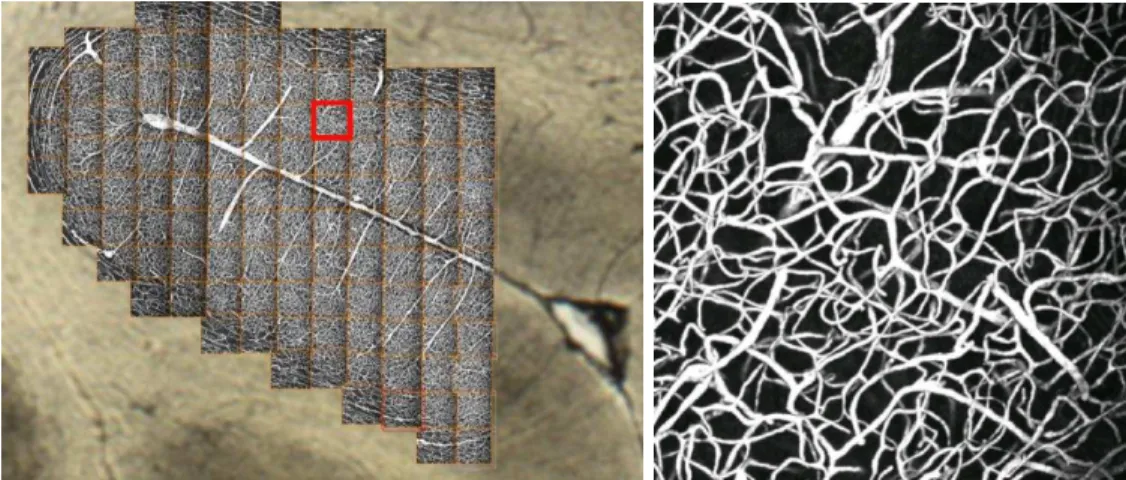
To image wider areas, an image mosaic has to be built (see Figure 2 (a)). The section is located on a table which can be translated with a micro-metric screw. Once an image is acquired, the section is translated, the acquisition of the next image is performed, and so on. The size of the area that can be so imaged is virtually unlimited. However, since the acquisition time is rather important (between 10 and 20 minutes per image), we limit ourselves to mosaics of about a hundred images, that already represented several mm2 of
(a) Image mosaic (about 7 × 7 × 0.2mm2
wide) (b) Maximum Intensity Projection (MIP) of one confocal image (600 × 600× 180µm3
wide, resolution: 1.2 × 1.2 × 1.4µm3
)
Figure 2: An image mosaic corresponding to the sulcus area of Figure 1 (b) and a sample of a single confocal image of this mosaic.
built of 118 images and covers about 7 × 7 × 0.2 mm3of the brain section. This corresponds
to a virtual image of approximately 6000 × 6000 × 128 voxels and 4 gigabytes.
2.2
Filtering
We then perform some filtering on each image, to improve the quality of the forthcoming thresholding. First, we perform a median filtering (3 × 3 × 3 kernel) to remove salt and pepper noise. Then, we perform a Gaussian filtering (3 × 3 × 3 kernel, σ = 1 voxel) to smooth borders. Filter parameters have been set empirically by experts. The figure 3 shows a portion of a mosaic image (a), after median filtering (b), and after Gaussian filtering (c).
2.3
Mosaic creation
Building a mosaic from several images requires the knowledge of their relative position from each other. This position is given by the micro-metric screw when displacing the imaged section under the microscope. However, some imprecision occurs between the real displacement and the value indicated by the screw, and moreover, the induced errors are cumulative. Thus, an automated repositioning is required.
(a) Original image (b) After median filtering (c) After Gaussian filtering
Figure 3: MIP of a part of an image mosaic before and after filters.
To achieve a precise relative positioning of the mosaic images, we design the acquisition protocol so that there is an overlap of about 50 voxels between two adjacent mosaic images. This overlap allows to use standard registration methods [MV98]. We restrict for the search of a 3-D translation that is computed by two successive steps.
• First, the in-plane (along X and Y directions) translation is considered. It is computed by optimizing a similarity measure on the overlapping area. In our case, a simple Sum of Squared Differences (SSD) appears to be enough. For computational purposes, we perform this step by considering the Maximum Intensity Projection (MIP) of the images.
• Second, the in-depth translation is considered. Such a translation occurs when the imaged section is not perfectly orthogonal to the optical axis of the microscope. Here, the computation is conducted with the overlapping 3-D parts of the images. We also use the Sum of Squared Differences as similarity measure.
The mosaic of confocal image stacks are merged into one large dataset comprising the whole examination volume. The value of a voxel in the overlapping area is defined as a linear combination of the values of the corresponding voxels in the original images: weights depend on the distance to the image borders to ensure smooth transitions. We obtain a huge image (about 4 Gb for the example shown figure 2(a)), stored on hard disk and where the value of each voxel is known and unique. This allows to load any sub-volume for inspection or for processing.
Finally, we perform a global segmentation with a user defined threshold value. Although not optimal, we chose this segmentation method because it is extremely fast and simple (lots of better segmentation techniques exist, but are behind the scope of this paper). The influence of this choice will be discussed in section 6.2.
3
Medial skeleton
If we model each vessel by its centre line, we obtain a 1-dimensional set, which allows not only to efficiently visualize details of the whole network, but also to count the number of vessels, their lengths, and the number of their junctions. Moreover, if we model a vessel by a cylinder (or a cylinder set), and associate to each centre line point the smallest distance to the background, we obtain the vessel radius at this point.
3.1
Distance Ordered Homotopic Thinning
3.1.1 Recalls
To determine vessels centre lines, we can consider either medial axis or skeleton. Medial axis was introduced by Blum [Blu67] with an analogy to grass fire: he defined local axis as the locus of points at which the propagation fronts meet and extinguish. Calabi and Harnett [CH68] defined a medial axis as the set of centers of maximal disks of the object, where a disk is said to be maximal in an object if there are no other disks included in the object containing this disk. A medial axis can be defined as a set which is thin and centered within the object. The second approach, introduced by Hilditch [Hil69] and Kong and Rosenfeld [KR89] defines the skeleton of an object. A skeleton is thin and topologically equivalent to the object.
In our case, the topology is the most significant property we want to preserve to character-ize and model the micro-vascular network. We thus consider homotopic skeletons. Moreover, as we also aim at computing vessels diameters, we want the skeleton to be centered within vessels. More precisely, we want the following properties to be verified.
homotopy: the skeleton is topologically equivalent to the original image. Particularly, it has the same number of connected components, holes and cavities as the original image.
thickness: the skeleton is thin i.e. one voxel wide. For discrete objects, however, it may happen that connectivity requires a two-voxel thickness at junction points. medialness: the skeleton is centrally located within the foreground object. As we are
dealing with discrete images, it may happen, in the case of an even voxels number, that a skeleton of one pixel wide cannot be exactly centered within the object. Some process, as for example compression, require the skeleton to be reversible, but this property is not essential for our application. As reversibility implies an additional cost, we will not consider it in this paper.
3.1.2 Existing methods to build a skeleton
A skeleton can be built in the continuous space through Voronoï diagrams or partial deriva-tive equations (PDE). In the case of the Voronoï diagram, the object outline is approximated
by a polygon [Ogn94]. The skeleton is defined as the subgraph entirely included within the object of the Voronoï diagram of this polygon vertices. In the case of PDE, the skeleton is defined as a zero or non-defined level-set of an evolutive surface (for example, the distance function to the background) [GF99]. Continuous methods lead to topological, centered and thin skeleton. However, they often rise difficulties when translated from the continuous to the discrete space. Moreover, the algorithm complexity and the computational time are crippling for huge images.
This leads us to considering discrete methods which are generally fast and easy to use. Such methods can then be based on:
thinning: the skeleton is computed by iteratively peeling off the boundary of the object, layer-by-layer. Thinning process use the notion of simple points. A point is said to be simple if its deletion preserves the object topology. Such a point can be characterized by considering the topology of its neighborhood [BM94]. Thus, thinning methods con-sist in deleting only simple points (to be sure to preserve topology). If all simple points are removed iteratively, the result object is topologically equivalent to the original one, but far too simple: a connected component without hole nor cavity will be shrunk to a single point. Conditions for end points are defined for points located on the border of a line or surface to keep it a line or a surface. Indeed, thinning process remove deletable points (i.e. simple points that are also border points and non-end points) either sequentially [PSBK01], or in parallel [TF81, GB90, PA99, MW00, LB02], or with morphological operations [Jon00]. These methods lead to a skeleton which is homotopic to the object, by construction, thin and geometrically representative (if the end-points have been correctly characterized), but not necessarily centered.
distance maps: the skeleton is defined as the locus of the local maxima of the distance map [CH68, MF98, ZKT98]. The principle of these methods is to calculate the distance map of the object, to find local maxima and to re-connect these maxima. The resulting skeleton is centered by construction, thin, depending on the local maxima threshold, but not necessarily homotopic.
Hybrid methods have been recently introduced to take advantage of both approaches [ST95, Pud98]. These methods are called Distance Ordered Homotopic Thinning (DOHT). They use a distance map to guide the process of iteratively removing simple points (ho-motopic thinning) towards the centre of the object. They thus lead to a skeleton which is homotopic to the original object (because only simple points are deleted), thin (because points are deleted until no deletable point is found), and as centered as possible (because point deletion follows the distance to the background).
Since the DOHT methods exhibit the properties we request for our skeleton, it will be our method of choice.
3.2
Distance map
DOHT algorithms require the computation of a distance map of the object to skeletonize. A distance map is a grey level image where the value of each object point corresponds to its shortest distance to the background. Numerous ways have been investigated to compute dis-tance maps. Chamfer transforms, popularized by [Bor84], achieve a good trade-off between precision and computational cost. They propagate local integer distances using chamfer masks. Roughly speaking, a chamfer mask is a set of legal displacements weighted by local distances. Figure 4 (a) shows an example of a 2D 3 × 3 chamfer mask. For a 2D (3D)
(a) Parallel chamfer mask (b) Iterative masks
Figure 4: Samples of 2D 3 × 3 chamfer masks.
image, we note Ii, Ij (and Ik) the image dimensions in ~x, ~y (and ~z) direction. Rosenfeld
and Pflatz [RP66] have shown that a distance map can be computed with two scans on the image: a so-called forward scan from the top left corner of the image (point of coordinates (1, 1)) to the bottom right corner of the image (point of coordinates (Ii, Ij)), and a backward
one, from the bottom right corner of the image (point of coordinates (Ii, Ij)) to the top left
corner (point of coordinates (1, 1)) of the image. To do so, the image is first initialized to 0 for the background and ∞1 for the object points. Then, they use half masks (cf. figure 4
(b)) and affect to each object point the minimum value between its previous value, and the 1Practically a very high value.
value of the points located in its half neighborhood added with the corresponding weight of the half-mask. Thus, during the forward scan, the value of the current point depends on its neighbors located on its left and above (right and left) of this point. In the same way, during the backward scan, the value of the current point depends on its neighbors located on its right and under (right and left).
This algorithm can be easily adapted to higher dimension. For example in 3 dimensions, the 3 × 3 × 3 forward chamfer mask of a point (i, j, k) ∈ Z3contains the following weighted
points: ( i-1, j-1, k-1), ( i, j-1, k-1 ), ( i+1, j-1, k-1), ( i-1, j, k-1), ( i, j, k-1 ), ( i+1, j, k-1), ( i-1, j+1, k-1), ( i, j+1, k-1 ), ( i+1, j+1, k-1), ( i-1, j-1, k ), ( i, j-1, k ), ( i+1, j-1, k ), ( i-1, j, k ),
and the forward scan writes as follows for each point p(i, j, k) ∈ I:
1: fork= 1 to Ik do
2: forj= 1 to Ij do
3: fori= 1 to Ii do
4: I(p) = min~v∈f orward_mask(I(p), I(p + ~v) + ω~v)
A distance between two points is generally defined as the length of the shortest path between these points. In the case of chamfer distance, we reduce the path choice to linear combinations of the legal displacements allowed by the mask. To obtain a chamfer distance as close as possible to the Euclidean one, we can, on one side, allow more paths, which means increasing mask size, and, on another side, carefully choose the mask coefficients leading to the smallest error with respect to the Euclidean distance. The first way is the easiest one, but it increases the chamfer map computational cost. The second one it the most challenging one. This computation is generally done on isotropic grids. In our case, however, slice thickness is larger than pixel size. Dealing with an isotropic grid would lead to interpolate data and to drastically increase the amount of data. This is undesirable for the aimed application. In order to prevent such problem, we take into account the anisotropy of the lattice and consider the use of adapted coefficient computation methods [FM05].
4
Blockwise processing
The algorithms presented in the previous section implicitly assume that the image can be loaded and processed at once in the memory of the computer. This is not the case for our images. We decided to process the image by sub-images or blocks. Moreover, to ensure a correct propagation of local distances as well as a correct extraction of a homotopic and centered skeleton, these algorithms have to be carefully re-designed.
4.1
Synthetic images
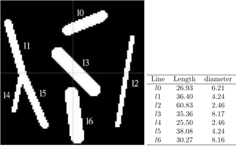
To illustrate the problems raised by a block-wise process, and to test our algorithm validity, we produced a synthetical image. We consider a 100 × 100 × 50 voxels binary image. To simplify comparisons, we choose to create an isotropic image (1 × 1 × 1 voxel size). This image is small enough to be entirely processed at once, but we will also process it in 4 blocks to compare the results we obtain with the result obtained when processed as a single image. We draw lines in this image with known coordinates through Bresenham’s algorithm, and dilate the lines with spherical structuring elements of several known diameters.
Figure 5(a) shows the obtained image, and table 5(b) sums up the different coordinates and diameters of lines. We can notice that diameters are not integers. This is due to the
(a) Synthetic image
Line Length diameter l0 26.93 6.21 l1 36.40 4.24 l2 60.83 2.46 l3 35.36 8.17 l4 25.50 2.46 l5 38.08 4.24 l6 30.27 8.16
(b) Original lengths and di-ameters
Figure 5: Synthetic image and coordinates.
fact that the structuring elements we use are not real spheres, but discrete elements. This results in the fact that the shortest distance to the background is located at the corner of a voxel.
4.2
Blockwise distance map
If we compute distance maps independently on each image block, we obtain wrong values at block borders. Indeed, figure 6(left) shows the result of the forward scan computed by
Figure 6: From left to right: propagation resulting from a 2-D forward scan; propagation resulting from a naive blockwise 2-D forward scan (each block is considered once); propaga-tion resulting from an adequate blockwise 2-D forward scan (each block is considered twice, except the blocks at the end of block rows that are considered once).
considering only one block for the mosaic, and figure 6(center) shows the result of the forward scan by considering sequentially the blocks of the mosaic.
Two reasons explain this behavior:
• First, local distances should be propagated from a block to another through chamfer masks. To do so, blocks must overlap each other. The overlap size depends on mask size. For example, for a 3×3×3 chamfer mask, block must have at least one overlapping voxel in each direction (2 voxels for a 5 × 5 × 5 mask and so on). Figure 6(center) is computed with such an overlap.
• Second, to update a point value, for example in the forward scan, the process must know the value of its neighbours located on the left, above (on the left and on the right), and in the previous plane (above, under, on the left and on the right). In the case of a point located on the right border of the first block, points located on its right (above and on the previous plane) are not updated yet. A simple forward scan on each block from up left to bottom right is thus not enough. This is depicted by figure 6(center). It is the same for points located on left border block for the backward scan. A simple backward scan on each block is not enough either.
To overcome these problems, we divide the image into overlapping blocks, and we perform several scans on rows of blocks, columns of blocks and planes of blocks. Indeed, in the forward scan, once a row of blocks has been forward processed from left to right, we perform another forward process on this row of blocks, but from right to left (as depicted by figure 6(right)), to update right border points of each blocks (except for the block located on the right border of the row which doesn’t need to be updated). In the same way, once a plane of blocks has been processed from top to bottom, we perform forward process from bottom to top on this plane of blocks to update points located on the bottom border of blocks (to update a point located on a bottom border of a block, values of points located under this
points, in the previous plane, are needed and not yet updated). We perform the same way for the backward scan.
4.3
Blockwise skeletonization
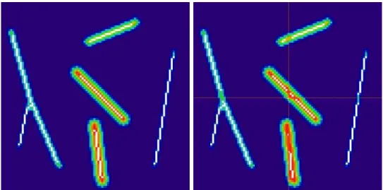
Blockwise skeletonization process also rises problems. Figure 7 (a) shows the skeleton we would obtain by processing the whole image at once. Figure 7 (b) shows the skeleton we obtain by independently processing each block. We can observe that disconnections appear at each block border.
(a) Skeleton obtained on the whole image (b) Skeleton obtained on each block pro-cessed independently
Figure 7: If we process independently on each block, disconnections appear on each block border.
Few authors propose tools to compute blockwise centerlines extraction. For example, Vossepoel et al. [VSD97] process independently on partially overlapping blocks, and then, re-connect skeleton parts within the overlapping areas. However, to be able to know which point has to be re-connected with an other, a previous labeling of each object to be skeletonized is required. In our application, labeling each vessel is simply not realistic. Pakura et al. [PSA02] use mask driven skeletonization to determine nervous fibers on partially overlapping sub-blocks. Unfortunately, as skeleton location is not mandatory for their application, no precautions are taken to center skeletons within fibers located at block borders.
We propose to adapt distance ordered homotopic thinning to a block-wise process. This adaptation is driven by the skeleton properties we want to preserve: homotopy, medialness and thinness.
4.3.1 Homotopy
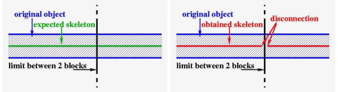
Homotopy can be guaranteed by deleting only simple points of the object. A point can be guaranteed to be simple by investigating its neighborhood [BM94]. Problems of homotopy (vessels disconnections creating new connected components) may appear on block borders. Indeed, neighborhoods of points located on block borders are partially unknown. On one hand, if we assume that the unknown neighbors belong to the background, the object to be thinned can be disconnected from the border, and disconnections will appear on block borders. On the other hand, if we assume that these unknown neighbors belong to the fore-ground, the object to be thinned can not be disconnected from the border, but the resulting thinned object (in the whole mosaic) can be disconnected as well since the continuity of the skeleton from block to block is not ensured.
Figure 8 (a) shows the example of a vessel located across 2 blocks and the skeleton expected for this vessel. Figure 8 (b) shows the skeleton obtained when the two blocks are processed independently.
To solve this problem, we freeze points located on block borders, i.e. we consider points as deletable only if the whole neighborhood is included within the block.
This condition guarantees a homotopic skeleton. Indeed, changes of homotopy (e.g. disconnections) appear when considering each block independently because some points located on block borders are not simple points in the whole mosaic, but appear to be simple with respect to one block as their neighborhood is not entirely known. Freezing border points ensure that each deleted point is simple with respect to the whole mosaic (because the neighborhood is of each point within one block is entirely known). By definition of simple point, deleting simple points does not alter the object topology.
However, one may notice that thick portions of the object appear at the borders. They will be be later deleted by further considering other blocks that straddle the borders. 4.3.2 Medialness
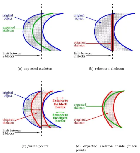
As opposed to properties that can be ensured locally, e.g. homotopy with the sequential delatin of simple points, medialness is a regional property which is more difficult to guaran-tee, and that is no more verified if we only freeze points on the on-voxel border as proposed above. Indeed, if we delete all simple points except for the border of a block, the skeleton may be mislocated.
As shown in figure 9 (a) and (b), some points expected to be in the skeleton can be deleted. The connected component kept from the object becomes the “frozen” points of the border.
The skeleton is then “stucked” to the border of the first thinned block and not located at the object center. To overcome this problem, we consider points to be deletable only if their
(a) expected skeleton (b) independent computation of each block: the skeleton is disconnected on block borders.
(c) border points “freezing” guaranties the skeleton connectivity across borders.
Figure 8: Exemple of homotopy problems on block borders. The blue vessel crosses 2 blocks. If we process each block independently, its skeleton will be disconnected.
distance to the block border is larger than their distance to the object border (see figure 9 (c)). This means that a point can be deleted only if its associated maximal ball is entirely included within the block, or equivalently that points that do not verify this property have to be “frozen” to prevent them to be deleted.
This last property locally adapt the shape of the “frozen” part of the object on borders to ensure that points of the expected skeleton will not be deleted at this phase. Figure 9 (d) shows the object component which is kept after this skeletonization phase.
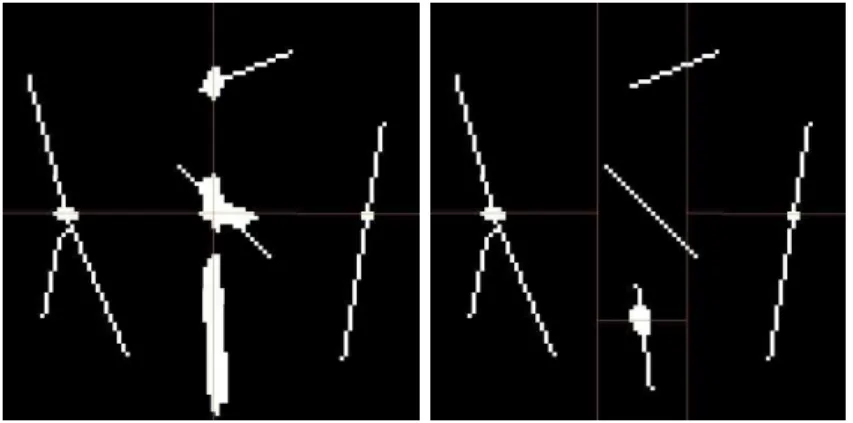
Figure 10 (a) shows the result of the skeletonization process applied to the synthetic lines (cf figure 5 (a)), taking into account these two conditions.
The expected skeleton is located within this component, but it is not really centered. To this end, as shown in the next section, we will apply another skeletonization phase
(a) expected skeleton (b) relocated skeleton
(c) frozen points (d) expected skeleton inside frozen points
Figure 9: Exemple of skeleton relocation problem. If we freeze only border points, the skeleton is “stucked” to the block border.
on this area. Simple points deletion will be ordered by the original object distance map. The correct skeleton will be located on this distance map maxima, and the skeletonization algorithm will delete every point located around these maxima before reaching the expected skeleton points. This will lead to a medial skeleton.
4.3.3 Thinness
The two previous conditions lead to a homotopic (because we remove only simple points) and potentially medial (bacuse points located on maximal balls centers are not deleted) skeleton. But it may remain thick. Indeed, object areas located on block borders have not entirely been thinned. To obtain a thin skeleton, we re-apply the skeletonization algorithm with the same conditions, but on the area remained thick, that is to say the block border areas. To do so, blocks are re-designed as thick strips centered on previous block borders. The strip thickness depends on the largest distance found in the mosaic. As we are dealing with vessels, we are sure that the largest vessel diameter is far smaller than a block width. Figure 10 (b), (c) and (d) shows different scans in vertical and horizontal direction. As we are dealing with 3D images, we perform the same way in z-direction.
This blockwise thinning skeletonization methodology ensures that most of the mosaic will only be accessed once, while only a small part of the mosaic (the points inside the additional strip blocks on the border) will be accessed several times. This way, the additional cost due to the blockwise processing is somewhat minimized.
We thus obtain a skeleton which is homotopic to the original object, as centered and as thin as possible with respect to the definition given in the previous section.
5
Results
Once distance map and skeleton are computed, we:
• convert the binary image obtained in a lines network, by considering points connec-tivity. This allows us not to store a huge binary image, but only connected lines with the coordinates of each of their points.
• affect to each line point the corresponding distance found in the distance map, which gives us the vessel radius on each point of its centre line (and allow to compute its mean diameter).
In this way, as a line models a vessel, we have direct access to vessels number, lengths, and mean diameters.
5.1
Synthetical data
Table 1 presents the lengths and mean diameters we obtained on synthetical data presented figure 5.
If we except lines l1, l4 and l5, we can notice that lengths are always under-estimated (of about 15%). This is due to the fact that during skeletonization process, several points are deleted before a line end-point appears. Indeed line end-points definition moves objects border toward its center (cf figure 7 (a)). In the case of lines l1, l4 and l5, values differ because the junction point between these three lines have been relocated when we performed
(a) 1rst step: process on inde-pendent contiguous blocks
(b) 2nd step: process borders on vertical direction
(c) 3rd step: process borders on horizontal direction
(d) last step
Figure 10: Steps of figure 5 (a) skeletonization using our method. In the first step of block-wise skeletonization, contiguous blocks are processed (border points are freezed according to previous conditions). Then border blocks are processed in x, y and z direction (for visualization issue, we see here only planar process).
a dilation on Bresenham lines to give them a diameter. This, added to the relocation of line borders gives higher errors.
Line Length error (%) diameter error (%) l0 23.31 13.4 6.059 2.4 l1 38.73 6.4 4.195 1.1 l2 52.73 13.3 2.338 5.1 l3 29.70 16.0 7.700 5.7 l4 17.8 29.8 2.401 2.6 l5 35.80 32.2 4.167 1.8 l6 25.66 15.2 8.130 0.4
Table 1: Lengths and diameters obtained with our method for synthetic lines (cf Figure 5). Concerning diameters, they are systematically under estimated too. But the error never exceeds 6% which agrees with values proposed in [FM05] and proves that the skeleton is correctly centered.
5.2
Real data
We integrated these algorithms into the visualization system Amira [Zus03]. The experimen-tations were conducted on a Pentium 4 at 1.7GHz laptop with 512M b RAM. The amount of data (4 Gb for the original image, plus 4 Gb for the segmented image, plus 8 Gb for the distance map (stored on short integers, as bytes are not enough to store the result of chamfer map), and 4 Gb for the skeleton creation image, i.e. 20 Gb for the whole process) leads us to store result images on a distant hard disk, which slowed down the image read/write process, and considerably increase the total computational time.
Computing chamfer distances takes 13min of actual calculation, and 14h17min of total process due to images read/write artifacts. Skeletonization process takes 1h32min of actual calculation for a total duration of 8h08min for the whole mosaic. During these two processing steps, the mosaic was cut into about 256 × 256 × 128 voxel sub-images (the number of voxels may slightly change considering block location, e.g. blocks located on the border of the mosaic, and overlap needed between blocks). The whole process takes then several hours on a standard PC, mostly due to I/O procedures, but it remains comparable to the total acquisition time of the mosaic.
After converting the voxel representation of the skeleton to a geometric representation of lines, the result can be interactively explored. Displaying the original image data together with the generated skeleton in one visualization is possible (see figure 12 (a)). This helps to verify as well as to document results.
Figure 11 shows vessels center lines obtained from the image shown in Figure 2. The whole lineset contains more than 2,000,000 points and about 74,000 lines.
From these data, we can also extract statistical data, as, for example histogram of vessels radii (see figure 12 (b)). We can notice than most vessels radii are lower than 10µm, with a peak at about 5µm.
Figure 11: Vessels center lines network of the mosaic presented figure 2.
6
Discussion
6.1
Validation
Validation is a critical issue in medical imaging process. We performed a qualitative valida-tion on real data and a quantitative validavalida-tion on simulated images.
6.1.1 Qualitative validation on real images
The first aim of our study was a proof of feasibility. We showed that extracting morphome-trical data on real data representing several square millimeters of he brain was feasible in reasonable time (at least in finite time). This study allowed to recover several qualitative results showed by anatomists [DSV81]:
• the shape of vessels junctions corresponds to their expectations: veins and arteries emerge from the cortex with right angles, and form sharp angles in deep layers. • the distribution of vessels density corresponds to the observation on several cortex
layers.
(a) vessels modeled as cylinders sets (b) Distribution of vessels radii
Figure 12: Visualization of results obtained on the mosaic presented figure 2.
Unfortunately, this validation on real data cannot be quantitative as we are not aware of a ground truth set of morphometrical values on such data.
6.1.2 Quantitative validation on synthetic binary image
We produced synthetic binary image to test our block-wise processing methods. We showed that we obtained a skeleton which is homotopic, thin and centered with respect to the binary object. Moreover, we showed that vessels diameters where estimated with an error smaller or equal to 6%. This validation on synthetic data did not take into account the segmentation step. Indeed, the purpose of this paper is to propose block-wise processing methods to work on huge images.
6.2
Dependance on segmentation
By construction, the obtained skeleton is topologically equivalent and centered with respect to the binary object.
We observe that the number of spurious branches that may appear in thinning processes is considerably reduced by both distance map consideration and a directional strategy. Indeed, spurious branches correspond to low values of distance map and are generally scattered all around vessels. Moreover, Gaussian filtering, performed before segmentation, smoothes borders and reduces irregularities that may lead to such spurious branches.
(a) threshold value: 40 (b) threshold value: 50
(c) threshold value: 60
Figure 13: Radii histograms considering several threshold values.
However, being topologically equivalent to the binary object leads the skeleton to highly depend on segmentation, and on the threshold choice. For example, if binarization creates a hole within a vessel, then the skeleton will get around this hole to be topologically equivalent to the segmented object.
Additionally, the final result may depend on the threshold choice. Indeed, the higher the threshold value is, the less points are taken for each vessel, and the smallest there mean diameters are. Conversely, the lowest the threshold value is, the most points are taken for each vessel and the highest there mean diameter is.
Figure 13 shows a zoom on vessels radii histogram of the same mosaic processed with a threshold of 40 (a), 50 (b) and 60 (c)2. We can observe that these histograms have the same
overall shape, but radii values are slightly shifted form one threshold value to another. We are 2Values of original images vary between 0 and 255. Inter and intra-operator variability for the choice of
conscious that a particular attention must be paid for binarization. On-going work on a more accurate segmentation, better adapted to our specific data (e.g. histogram equalization, mathematical morphology...), is currently conducted. We favor automatic segmentations techniques which limit inter and intra-operator variations.
However, it has to be pointed out that vessels shapes and diameters have been con-siderably altered by the preparation process. Indeed, vessels may have been inflated by Indian ink injection, distorted by the cutting process, and flattened between the slide and the cover-glass to be observed with a microscope. The imprecision brought by the choice of the binarization threshold is less important with respect to the deformations vessels were subjected to.
7
Conclusion and Perspectives
The extraction of morphometric parameters from a mosaic of 3-D confocal microscopic images has been presented. This has required the design and development of dedicated software tools. Indeed, as huge images cannot be loaded at once in a standard computer memory, they need adapted algorithms. We chose adapted data structures allowing block-wise computation. Our block-block-wise skeletonization method preserves global as well as local skeleton properties by avoiding border effects. In a first pass, we process 3D blocks without overlapping. Next, we process images covering boundaries. The size of these sub-images depends on the size of the object to be thinned. Doing so, inner block areas are processed only once. The algorithm overhead due to the block by block process appears only on boundaries. We have also shown that for our application, our tools allow to extract quantitative information precious for neuro-anatomists and neuro-physiologists to describe the brain micro-vascular network.
This application can be widen to other acquisition techniques (as long as it can lead to a binarized image with vessels outlined from the background), and to other research area (e.g. oil industry or plant roots study [KFPM04]). Indeed, the presented technics can be applied to any binarized large data, as long as considered objects represent tubular structures or smqll shapes with respect to the size of a block to ensure that we can design strips at block borders for the skeletonization.
Moreover, block-wise process can be used for distance map or skeletonization paralleliza-tion.
References
[BGPA03] E. Bullitt, G. Gerig, S.M. Pizer, and S.R. Aylward. Measuring tortuosity of the intracerebral vasculature from MRA images. IEEE Transactions on Medical Imaging, 22:1163–1171, 2003.
[Blu67] H. Blum. A transformation for extracting new descriptors of shape. Models for Perception of Speech and Visual Form, pages 362–380, 1967.
[BM94] G. Bertrand and G. Malandain. A new characterization of three-dimensional simple points. Pattern Recognition Letters, 15(2):169–175, February 1994. [Bor84] G. Borgefors. Distance transformations in arbitrary dimensions. Computer
Vi-sion, Graphics, and Image Processing, 27:321–345, February 1984.
[CDM99] O. Craciunescu, S.K. Das, and Dewhirst M.K. Three-dimensional microvascular networks fractal structure: A potential for tissue characterization? In Advances in Heat and Mass Transfer in Biotechnology, HTD, volume 363, pages 9–13, 1999.
[CH68] L. Calabi and W.E. Harnett. Shape recognition, prairie fires, convex deficiences and skeletons. American mathematical monthly, 75:335–342, 1968.
[DSV81] H.M. Duvernoy, S. Selon, and J.L. Vannson. Cortical blood vessels of the human brain. Brain Research Bulletin, 7(5):519–579, November 1981.
[FL01] E. Farkas and P.G.M Luiten. Cerebral microvascular pathology in aging and Alzheimer’s disease. Progress in Neurobiology, 64:571–611, 2001.
[FM05] Céline Fouard and Grégoire Malandain. 3-d chamfer distances and norms in anisotropic grids. Image and Vision Computing, 28(2):143–158, February 2005. [FMP+04] C. Fouard, G. Malandain, S. Prohaska, M. Westerhoff, F. Cassot, C. Mazel,
D. Asselot, and J.-P. Marc-Vergnes. Skeletonization by blocks for large datasets: application to brain microcirculation. In International Symposium on Biomedical Imaging: From Nano to Macro (ISBI’04), Arlington, VA, USA, April 2004. IEEE.
[GB90] W. Gong and G. Bertrand. A simple parallel 3D thinning algorithm. In Inter-national Conference on Pattern Recognition, pages 188–190, 1990.
[GF99] J. Gomes and O. Faugeras. Reconciling distance functions and level sets. Tech-nical Report RR-3666, INRIA, 1999.
[Hil69] C.J. Hilditch. Machine Intelligence, volume 4, chapter Linear skeletons from square cupboards, pages 403–420. Edinburgh University Press, 1969.
[HR02] D.J. Heetger and D. Ress. What does fMRI tell us about neuronal activity? Nature Reviews Neuroscience, 3:142–151, February 2002.
[Jon00] P.P. Jonker. Morphological operations on 3D and 4D images: From shape prim-itive detection to skeletonization. In Discrete Geometry for Computer Imagery, volume 1953, pages 371–391. Springer, 2000.
[KFPM04] P. Kolesik, C. Fouard, S. Prohaska, and A. McNeill. Automated method for non-destructive 3D visualisation of plant root architecture using X-ray tomography. In 4TH International Workshop on Functional-Structural Plant Models, page 27, Montpellier, France, June 2004. UMR AMAP/CIRAD.
[Kle01] D. Kleinfeld. Cortical blood flow through individual capillaries in rat vibrissa S1 cortex: Stimulus induced changes in flow are comparable to the underlying fluctuations in flow. In Tomita, editor, Proceedings for Brain Activation and CBF Control, June 2001.
[KR89] T.Y. Kong and A. Rosenfeld. Digital topology: Introduction and survey. Com-puter Vision, Graphics, and Image Processing, 48:357–393, 1989.
[LB02] C. Lohou and G. Bertrand. A new 3D 6-subiteration thinning algorithm based on p-simple points. In Discrete Geometry for Computer Imagery, volume 2301, pages 102–113. Springer, 2002.
[LHH+93] S. Lai, A.L. Hopkins, E.M. Haacke, D. Li, B.A. Wasserman, P. Buckley, L.
Fried-man, H. Meltzer, P. Hedera, and R. Friedland. Identification of vascular struc-tures as a major source of signal contrast in high resolution 2D and 3D functional activation imaging of the motor cortex at 1.5T: Preliminary results. Magnetic Resonance in Medicine, 30(3):387–392, September 1993.
[MF98] G. Malandain and S. Fernández-Vidal. Euclidean skeletons. Image and Vision Computing, 16(5):317–327, April 1998.
[MV98] J.B.A. Maintz and M.A. Viergever. A survey of medical image registration. Medical Image Analysis, 2(1):1–36, March 1998.
[MW00] C.M. Ma and S.Y. Wan. Parallel thinning algorithms on 3D (18, 6) binary images. Computer Vision and Image Understanding, 80:364–378, 2000.
[Ogn94] R.L. Ogniewicz. Skeleton-space: a multiscale shape description combining re-gion and boundary information. In Computer Vision and Pattern Recognition (CVPR’94), pages 746–751, Seattle, USA, June 1994. IEEE.
[PA99] Kálmaán Palágyi and Kuba Attila. Directional 3D thinning using 8 subitera-tions. In Discrete Geometry for Computer Imagery, volume 1568, pages 325–336. Springer, 1999.
[PSA02] M. Pakura, O. Schmitt, and T. Aach. Segmentation and analysis of nerve fibers in histologic sections of the cerebral human cortex. In Processing of the Fifth IEEE Southwest Symposium on Image Analysis and Interpretation (SSIAI’02), pages 62–66, Santa Fe (New Mexico), 2002.
[PSBK01] Kálmaán Palágyi, Erich Sorantin, Emese Balogh, and Attila Kuba. A sequential 3D thinning algorithm and its medical applications. In Information Processing in Medical Imaging (IPMI 2001), volume 2082, pages 409–415. Springer-Verlag, june 2001.
[Pud98] C.J. Pudney. Distance-ordered homotopic thinning: A skeletonization algorithm for 3D digital images. Computer Vision and Image Understanding, 72(3):404– 413, December 1998.
[RP66] A. Rosenfeld and J.L. Pfaltz. Sequential operations in digital picture processing. Journal of the Association for Computing Machinery, 13(4):471–494, October 1966.
[ST95] T. Saito and J.i. Toriwaki. A sequential thinning algorithm for three dimensional digital pictures using the euclidean distance transformation. In 9th Scandina-vian Conference on Image Analysis (SCIA’95), pages 507–516, Uppsala, Sweden, June 6–9 1995. IAPR.
[TF81] Y.F. Tsao and K.S. Fu. A parallel thinning algorithm for 3-d pictures. Computer Graphics and Image Processing, 17:315–331, 1981.
[Tur01] Robert Turner. How much cortex can a vein drain? downstream dilution of activation-related cerebral blood oxygenation changes. NeuroImage, 16:1062– 1067, October 2001.
[Vit01] Jeffrey Scott Vitter. External memory algorithms and data structures: Dealing with massive data. ACM Computing Surveys, 33(2):209–271, 2001.
[VSD97] A.M. Vossepoel, K. Shutte, and C.F.P Delanght. Memory efficient skeletoniza-tion of utility maps. In Proceedings of 4th Internaskeletoniza-tional Conference on Document Analysis and Recognition, pages 797–800, Ulm (Germany), 1997.
[ZKT98] Y. Zhou, A. Kaufman, and A. W. Toga. 3D skeleton and centerline genera-tion based on an approximate minimum distance field. Internagenera-tional Journal of Visual Computer, 14(7):303–314, 1998.
[Zus03] Zuse Institute Berlin (ZIB) and Indeed - Visual Concepts, Berlin. Amira 3.1 – User’s Guide and Reference Manual – Programmer’s Guide, October 2003. http://amira.zib.de.
Unité de recherche INRIA Futurs : Parc Club Orsay Université - ZAC des Vignes 4, rue Jacques Monod - 91893 ORSAY Cedex (France)
Unité de recherche INRIA Lorraine : LORIA, Technopôle de Nancy-Brabois - Campus scientifique 615, rue du Jardin Botanique - BP 101 - 54602 Villers-lès-Nancy Cedex (France)
Unité de recherche INRIA Rennes : IRISA, Campus universitaire de Beaulieu - 35042 Rennes Cedex (France) Unité de recherche INRIA Rhône-Alpes : 655, avenue de l’Europe - 38334 Montbonnot Saint-Ismier (France) Unité de recherche INRIA Rocquencourt : Domaine de Voluceau - Rocquencourt - BP 105 - 78153 Le Chesnay Cedex (France)