HAL Id: hal-02268350
https://hal.archives-ouvertes.fr/hal-02268350
Submitted on 20 Aug 2019HAL is a multi-disciplinary open access
archive for the deposit and dissemination of sci-entific research documents, whether they are pub-lished or not. The documents may come from teaching and research institutions in France or abroad, or from public or private research centers.
L’archive ouverte pluridisciplinaire HAL, est destinée au dépôt et à la diffusion de documents scientifiques de niveau recherche, publiés ou non, émanant des établissements d’enseignement et de recherche français ou étrangers, des laboratoires publics ou privés.
Teaching co-simulation basics through practice
Thomas Paris, Jean-Baptiste Wiart, Denis Netter, Vincent Chevrier
To cite this version:
Thomas Paris, Jean-Baptiste Wiart, Denis Netter, Vincent Chevrier. Teaching co-simulation basics through practice. 2019 SUMMER SIMULATION CONFERENCE, Jul 2019, Berlin, Germany. �hal-02268350�
Teaching co-simulation basics through practice
Thomas Paris
1, Jean-Baptiste Wiart
1,2, Denis Netter
2, and Vincent Chevrier
11
Universit´e de Lorraine, CNRS, LORIA, F-54000 Nancy, France
[email protected]
2
Universit´e de Lorraine, GREEN, F-54000 Nancy, France
[email protected]
July 2019
Abstract
Cyber-physical system representation is one of the current challenges in Modeling and Sim-ulation. In fact, multi-domain modeling requires new approaches to rigorously deal with it. Co-simulation, one of the approaches, lets modelers use several M&S tools in collaboration. The challenge is to find a way to enable co-simulation use for non-IT experts while being aware of assumptions and limitations involved. This paper deals with co-simulation basic principles teaching through practice. we propose an iterative and modular co-simulation process supported by a DSL-based environment for the MECSYCO co-simulation platform. Through a thermal use case, we are able to introduce co-simulation in a 4 hours tutorial destined to our students.
Keywords: Co-simulation, M&S Process, Teaching, CPS
1
CONTEXT
1.1
Energy Transition
Efficient energy management is one of this century challenges. The current trend to deal with it
is to build cyber-physical system (CPS) [Kleissl and Agarwal, 2010]. CPS are physical systems
monitored and supervised by one or several computers through a communication networks [
Ra-jkumar et al., 2010]. Smart-grids are examples of CPS where the energy network is coupled with a communication network to enable remote monitoring and control.
The Modeling and Simulation (M&S) of such systems is one of the current challenges in M&S due to the inter-disciplinary issues they raise. It requests the development of new methods which deal with multi-domain by integrating each expert point of view in the same rigorous and
efficient M&S activity. Co-simulation [Gomes et al., 2018] is a way to achieve it.
1.2
Co-Simulation
Co-simulation consists in modeling each part of the target system regardless of the others, in
heterogeneous models).This allows to simulate each model individually with the most appropri-ate simulator (M&S software) while ensuring the synchronization and exchange of data between these simulators.
It has several benefits. A first one is, from a modeler point of view, each part of the system can be modeled at the right level of abstraction in a dedicated M&S tool. A second one, from an industrial point of view, time and money can be earned by reusing existing specialized software instead of developing new ones.
Reusing models from several tools is an historical challenge, it was already a motivation for
the development of middleware like HLA [Dahmann et al., 1997]. For the last few years, we
can observe that co-simulation approaches to couple several M&S software is gaining interest in the industry. The Functional Mockup Interface (FMI) illustrates this interest. It is a growing
standard for model exchange and co-simulation between several M&S tools [Bertsch et al.,
2014].
However co-simulations still raises many challenges linked to technical (coupling software),
formal (coupling different simulator dynamics), validity and accuracy aspects [Schweiger et al.,
2019]. The practical aspect is also a hard task to achieve. It is still difficult to design a
co-simulation gathering the work of several partners, mainly because of IT required skills. Co-simulation is therefore an interesting method that needs to be taught, for the sake of rigorous use.
1.3
Teaching Background
ENSEM ( ´Ecole Nationale Sup´erieure d’ ´Electricit´e et de M´ecanique), one of the French ”Grandes
´
Ecoles” is an engineering school for students from the 3rd university grade to the 5th whose his-torical training consists of three major areas: mechanics, electrical engineering and IT systems. In the energy transition context, the school has oriented its teachings towards energy man-agement issues, including smart-grid M&S (and CPS in general). With the uprising interest in simulation in the industry, it became relevant to introduce our students with basic co-simulation knowledge. A dedicated introduction course of about 20 hours has been set up where students learn three kinds of modeling approaches (continuous, discrete event, and multi-agent systems) and co-simulation. Three sessions are dedicated to practice:
1. Discovery of NetLogo [Tisue and Wilensky, 2004],
2. Co-simulation basics with FMI and event handling on Java using JavaFMI [
Hern`andez-Cabrera et al., 2016], and
3. Co-simulation between FMI and Matlab on a thermal use case using theMECSYCO
plat-form [Camus et al., 2018] available onhttp://mecsyco.com/fr/. The paper focuses
on this session.
2
PURPOSE AND PROPOSAL
2.1
Goal
Academic or industrial projects are increasingly facing interdisciplinary issues that require greater cooperation between several domain experts. Co-simulation is one way to ease these collaborations but it requests an evolution on the way we think about M&S software. Co-simulation illustrates that modeling software should no longer be thought as closed systems
but rather as opened systems which can be reused in collaboration. Our purpose is to set up a class practice which introduces co-simulation, the basic principles and how it works. Problems related to continuous system co-simulation such as accuracy are mentioned during the course but not addressed in this tutorial in order to keep a guideline accessible .
2.2
Proposal
Based on our experience withMECSYCO, we propose an iterative and hierarchical procedure to
build multi-models and to design co-simulations. This procedure relies on the decomposition of the co-simulation process into 4 main steps: modeling, integration, multi-modeling and experi-ment. We relies on these steps to explain co-simulation principles. Moreover, a DSL (Domain Specific Language) based environment has been developed to support this process by enabling
co-simulation design from alreadyMECSYCOintegrated models without IT skills.
This work is our baseline to set up a co-simulation practice for our students on a thermal use case which contains:
• A simple house model designed with Modelica [Fritzson, 2011] and the BuildSysPro
library [Plessis et al., 2014], the model is exported as an FMU [Blochwitz et al., 2014],
version 2.0 of the standard. The idea is to show that we can use a state-of-the-art dedicated thermal library to define our models, in addition it let us introduce the FMI standard. • MatLab/Simulink for a simple controller model. MatLab is chosen because it is a
well-known tool for our students.
• A SQL database which contains real weather data collected during summer 2018 in Nancy. This database allows us to anchor our model in reality.
This practice highlights how co-simulation can help collaboration by enabling existing M&S software reuse while making students question the interoperability issues and the synchroniza-tion algorithm involved.
To sum up we propose a process to make students without much IT skills able to
perform MECSYCO co-simulations with several M&S tools (MatLab, FMI and an SQL
database) and to understand and question the way it works.
2.3
MECSYCO Background
MECSYCOis a DEVS wrapping platform (available onwww.mecsyco.comunder AGPL license)
that takes advantage of the DEVS universality [Zeigler et al., 2000] for enabling multi-paradigm
co-simulation of complex systems. It was used for the M&S of smart electrical grids in the context of a partnership between LORIA/Inria (French IT research institute) and EDF R&D
(main French electric utility company) [Vaubourg et al., 2015].
MECSYCO is based on the AA4MM (Agents & Artifacts for Multi-Modeling) paradigm [Siebert, 2011] (from an original idea of Bonneaud [Bonneaud, 2008]) that sees an heteroge-neous co-simulation as a multi-agent system. Within this scope, each couple model/simulator corresponds to an agent, and the data exchanges between the simulators correspond to the inter-actions between the agents. By following this multi-agent paradigm from the concepts to their
implementation, MECSYCOensures a modular, extensible (i.e. features such as an observation
system can be easily added), decentralized and distributable parallel co-simulation. MECSYCO
implements the AA4MM concepts according to DEVS simulation protocol for coordinating the executions of the simulators and managing interactions between models.
So far, we successfully define DEVS wrappers for discrete and continuous modeling tools
like the telecommunication network simulators NS-3 and OMNeT++ [Vaubourg et al., 2016],
the FMI standard [Blochwitz et al., 2014], and for the NetLogo simulator [Paris et al., 2017].
Entities fromMECSYCOrepresent co-simulation aspects. They are listed bellow:
• Model-artifact: They are responsible for the software and formal wrapping.
• M-agent: The dynamic part of the co-simulation, each agent is in charge of one model it controls through a model-artifact. They exchange data with each other using the coupling
artifacts and implement the Chandy-Misra-Bryant algorithm [Chandy and Misra, 1979]
for the co-simulation.
• Coupling artifact: They support the communication between agents, their use is similar to mailboxes.
• Model: These entities represent the integrated models and their simulators.
2.4
Four Steps Co-Simulation Process
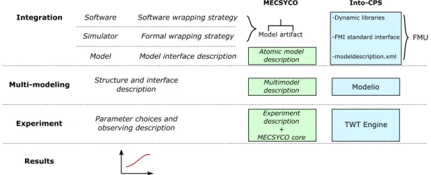
The Figure 1 represents our co-simulation design process (we assume solutions for both soft-ware and formal integration are already available). Note that these steps are not specific to
MECSYCObut can be applied to other co-simulation approaches, e.g. Into-CPS [Larsen et al.,
2016]. This scheme is used to locate the different steps of the co-simulation design.
Figure 1: From model components to co-simulations.
2.4.1 Modeling
The modeling step consists in developing the different components which will be used in the
experiment. Different formalisms and M&S software can be used. MECSYCOdoesn’t deal with
this step because it doesn’t provide means to write models, instead it proposes an approach to integrate models from different software, to connect them, and to co-simulate the resulting multi-model. Similarly, in the Into-CPS approach as in every FMI-based co-simulation tools, models to be used have to be designed in FMI compliant M&S software, i.e. software that can export FMU.
The modeling process ends with heterogeneous models which serve as inputs to integration process.
2.4.2 Integration
The purpose of the integration step is to transform the heterogeneous models into interoperable components. It requires at least a software and a formal integration, i.e. a way to exchange data between M&S software and to make simulators’ dynamics compliant.
InMECSYCO, the software and the formal integration are done through the development of a model-artifact in Java, outside the topic of the teaching, (this development requests DEVS knowledge and IT skills) while in Into-CPS this step is ensured by FMI which provides a stan-dard way to interact with the exported FMU.
In both case, the integration phase is completed by a model description file explaining the specific interface (parameters, inputs and outputs) of each model.
2.4.3 Multi-Modeling
Multi-modeling represents the coupling step. At this stage, we have the mean to use models
from several simulators (thanks to several model-artifacts in theMECSYCOcase), these atomic
models are described with XML files. We just have to define how models are coupled. Within theMECSYCOmiddleware, this job is done thanks to a multi-model description file whose shape
is inspired by the DEVS coupled structure [Zeigler et al., 2000] so we can design hierarchically
the final multi-model. In Into-CPS, this is done by using Modelio and the SysML notation.
2.4.4 Experiment
Last but not least, the co-simulation step consists in describing the experiment we want to perform (choice of multi-model, parameters and observing tools).
2.5
DSL Environment
One of the former MECSYCO drawback was the necessity to design the co-simulation as Java
code (it isn’t relevant for non computer scientist users). To fix it and support the co-simulation
process, a DSL-based environment for MECSYCOhas been developed using the XText
frame-work (seehttps://www.eclipse.org/Xtext/).
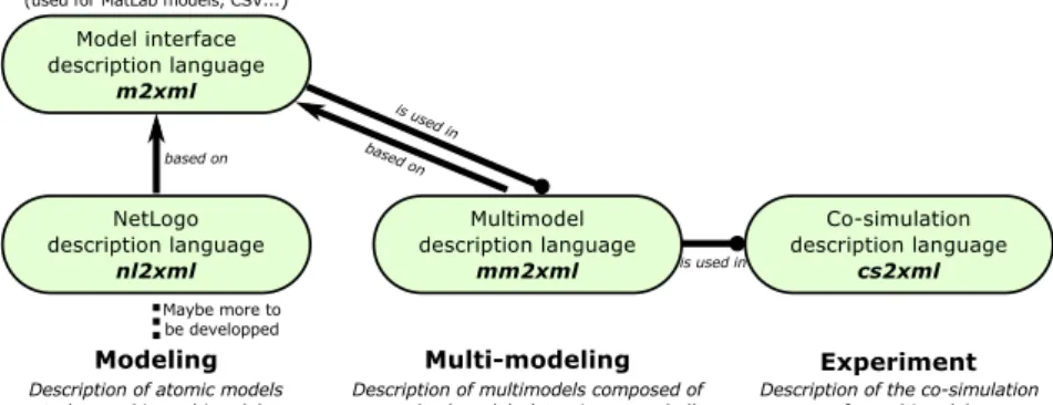
For each step, a dedicated DSL is implemented to ease the description phase (m2xml for atomic model interface, mm2xml for multi-model and cs2xml for experiment description). Fig-ure 2 shows the four DSL currently developed and their interactions (the nl2xml language is
dedicated to NetLogo model description [Paris et al., 2017]).
Note that mm2xml ensures modularity (changing a model by another consists in changing a path to another model/multi-model description) and hierarchical design (multi-model descrip-tions can be reused just like simple model descripdescrip-tions).
These DSL scripts generate XML files we can process to automate co-simulation launches.
With this new environment, MECSYCOcan be used to perform co-simulations without writing
a single line of Java code.
3
THE PRACTICE
The co-simulation process we explained before and the newly developed DSL-based
environ-ment forMECSYCOserve as a basis for a small co-simulation tutorial for students.
After a heat wave in Nancy 2018, we came up with the idea of studying how to use with effectiveness an air conditioner to maintain a comfortable temperature for a given house.
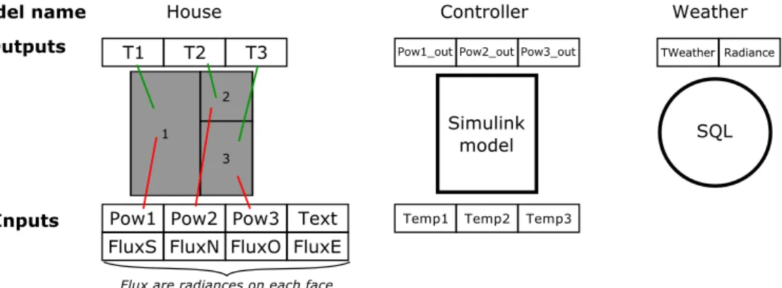
The system we want to model is a simple house composed of three rooms. Each room has its own air conditioner and influences the other rooms temperature through walls. The Figure 3 shows the three models we gave to our students to build the co-simulation. To keep it simple, we do not model explicitly the air conditioner but just its internal controller, i.e. the controller directly sends heat flows in the rooms. As we have limited time and focus on co-simulation, the students don’t build the models by themselves, we give them the different model components to connect.
Figure 3: Three components to co-simulate.
3.1
Details of the Models
3.1.1 House Temperature Model
The role of this model is to compute the temperature inside each room of the house depending on the weather condition (outside temperature and solar radiance) and on the power used to cool the house.
We explain just below the interface of this model:
• Parameters: They impact the insulation properties of wall (separation between inside walls and external walls), the volume of each room and each wall surface. They are not supposed to be changed during the class.
• Inputs: Pow1, Pow2 and Pow3 (in Joule per seconds) are the heat flows sent by the controller to regulate the house thermal behavior. Text represents the outside temperature
in Kelvin . FluxN, FluxE, FluxS and FluxO are the solar radiance (in Watt per m2) in
each cardinal direction.
This model is built with Modelica in OpenModelica [Fritzson et al., 2006] using components
from the BuildSysPro library developed by EDF R&D [Plessis et al., 2014]. Our goal with
BuildSysPro is to illustrate one interest of co-simulation: we can use state of the art library from one tool and use it in collaboration with other widely used M&S software.
3.1.2 Regulation Model
The regulation model is used to maintain a given temperature in a room. As our students are familiar with MatLab, we chose to build this model with MatLab/Simulink. We explain just below the interface of this model:
• Parameters: They concern the target temperature, the acceptable bandwidth and the maximum allowed power consumption for each room. We can also control the time step of the controller (the time between each order).
• Outputs: Three outputs Pow1, Pow2 and Pow3 (J.s−1) for each heat flow inputs of the
thermal model.
• Inputs: T 1, T 2 and T 3 (in Kelvin) are the temperatures of the rooms to control.
The controllers of the three rooms are contained in a single Simulink model, we could use three different models but keeping everything in a single one is more convenient. The model given to the student gathers three simple on/off controllers with hysteresis. One of the requested work is to propose something better and softer.
The interactions between theMECSYCO co-simulation platform and MatLab/Simulink are
enables by a model-artifact (a piece of Java code used for software and DEVS wrapping)
which relies itself on the free matlabcontrol library (see https://github.com/jakaplan/
matlabcontrol). Note that this model-artifact is the result of a student two month internship about MatLab integration, another approach would have been to export the MatLab model as an FMU.
3.1.3 Weather Data
We don’t use any model for the weather, instead, we use real data gathered during summer 2018. These data were collected by the Apheen (in english, Association for the accommodation of students and teachers of Nancy) in the context of a common project to study the thermal be-havior of their residences. To that purpose, they have collected data about outside temperature, wind speed and sunlight and stored them in a SQL database. In the co-simulation context, the weather component is seen as a source model, it only sends events to other models, i.e. there is no inputs. Then, its interface only contains:
• Parameter: There is one parameter, a time step which enables to control when the events are sent. Data are collected approximately every two minutes, the events send at a given date is either the record available at that time or the most recent record.
• Outputs: The two outputs we use in our example is TWeather (for the outside temper-ature, in Celsius), and Radiance (for the sunlight and in the building, only one wall is exposed to the sun).
The integration of this SQL database is also performed thanks to a model-artifact that loads all the data for a given period and then sent it as events at the requested times (depending on the chosen time step).
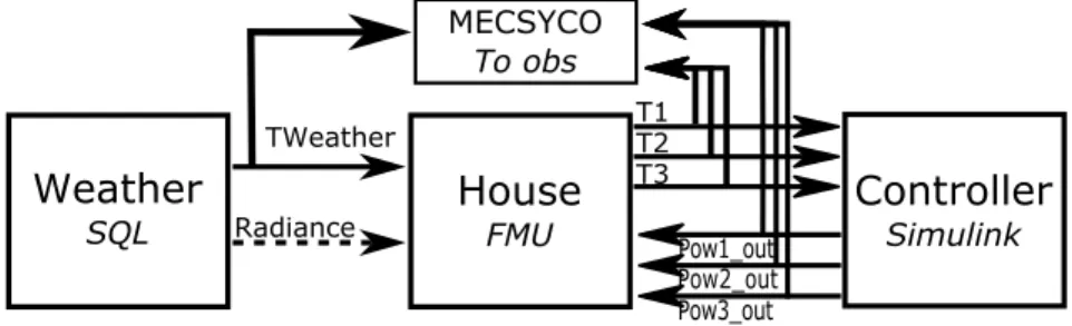
3.1.4 Target Multi-Model
The Figure 4 presents the multi-model students have to build and co-simulate from our three models (the radiance can, or not, be taken into account to measure its effect).
Figure 4: The multi-model to co-simulate.
3.2
Student Work
After a warm-up with Java code to see eachMECSYCOentity and to explain their role, students
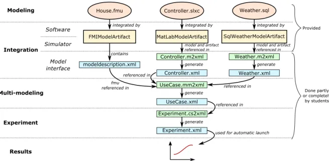
have to use the different DSL and examples available to design the co-simulation. Figure 5 sums up the process they follow. Each descriptive step shows what information is required to reuse an element. An important point to consider concerns the data representation when coupling heterogeneous models, e.g. in our multi-model, operations have to be applied during data transfer because temperatures in models are in Kelvin whereas they are in Celsius in the
database. These operations take place inMECSYCOcoupling artifacts and are specified during
the internal couplings descriptions.
We give DSL snippets which represent description of the controller in Figure 6 and partial description of the multi-model in Figure 7.
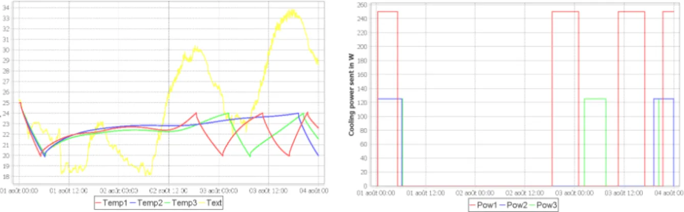
The results of the experiment are shown on Figures 8 and 9. The last question for our students is to review these results to make them wonder and discuss about the accuracy and validity of the models.
4
DISCUSSION
4.1
Related Works
The co-simulation process based on three descriptive steps (atomic model interface, multi-model and experiment) is inspired by the Into-CPS way of dealing with the co-simulation
process which was used for tutorials in the Sibiu CPS Summer school 2017 (see http://
projects.au.dk/into-cps/dissemination/summerschool/). The will to use descriptive files as supports for the modeling process is also motivated by various works like FMI (with
Figure 5: Summary of the co-simulation design process.
1 modelControllerMatlabtype”mecsyco.world.matlab.MatlabModelArtifact”
2 interface
3 parameters
4 maxTemp1:298.15 minTemp1:293.15 5 maxTemp2:298.15 minTemp2:293.15 6 maxTemp3:298.15 minTemp3:293.15 7 Temp1:294.15 Temp2:294.15 Temp3:294.15 8 Pow1:500. Pow2:0. Pow3:0.
9 maxPow1:500. maxPow2:250. maxPow3:250. 10 step:720. 11 inputs 12 Temp1:Double 13 Temp2:Double 14 Temp3:Double 15 outputs 16 Pow1_out:Double 17 Pow2_out:Double 18 Pow3_out:Double 19 information 20 keywords
21 ”Use case” ”TP” ”ENSEM” ”Smart heating” ”Controller”
22 description
23 ”Controller model of the TP ENSEM multimodel.”
24 simulator
25 simulation variables
26 stopTime:86400. timeStep:60.
27 dirPath:”U:\\Documents\\mecsycomatlab305\\workspace
28 \\MecsycoTpENSEMCorrection\\My Models\\matlab”
29 modelName:”controller”showMatlab:falseexitOnFinish:true
Figure 6: Overview ControllerMatlab.m2xml.
1 multimodelThermicUseCase 2 submodels
3 nameHousepath”My Models/fmu/House.fmu”
4 nameWeatherpath”Library/Basic/SqlModelWeather.xml”
5 nameControllerpath”Library/Basic/ControllerMatlab.xml”
6 interface
7 parameters
8 //Database
9 startDate:”2018−08−02”refers to(Weather:”startDate”) 10 endDate:”2018−08−05”refers to(Weather:”endDate”) 11 //Initial value for the House
12 Tinit:298.15refers to(House:”Tinit”) 13 TextInit:298.15refers to(House:”TextInit”) 14 //Represents the time between commands
15 step:720.refers to(Controller:”step”) 16 outputs
17 T1:Double refers to(House:”T1”)//... Same with T2, T3
18 Text:Double refers to(Weather:”TWeather”)
19 Pow1:Double refers to(Controller:”Pow1 out”)//... Same with Pow2, Pow3
20 internal couplings
21 {Weather.”TWeather”−> House.”Text”
22 event operation”model.operation.AddDoubleOperation”arg=273.15} 23 {Weather.”Radiance”−> House.”FluxS”}
24 {Controller.”Pow1 out”−>House.”Pow1”}
25 {House.”T1”−>Controller.”Temp1”}//...Same with FluxO, Pow2, Pow3, T2, T3
26 information
27 keywords”Use case” ”TP” ”ENSEM” ”Smart heating”
28 description”Example used to get ENSEM students
29 in touch with co−simulation concepts.”
30 simulator
31 simulation variables
32 stopTime:172800.refers to(House:”stopTime”)(Controller:”stopTime”) 33 (Weather:”stopTime”)
34 timeStep:60.refers to(House:”timeStep”)// Same with Controller
35 commStep:1refers to(House:”communicationStep”)
Figure 7: Overview UseCase.mm2xml. its modeldescription.xml) and HLA (with the Simulation Object Model). In the continuations of this work we plan to add other data in the descriptions (like physical units) and to provide analysis tools.
4.2
Next Steps
The models we define are not much accurate and have not been compared to real use case. However, this kind of multi-model can be used to determine the size of an air conditioner or reversible heat pump before installing it or to test different controller behaviors. Then a perspec-tive would be to test several controller models from several M&S tools (by taking advantage of
Figure 8: Evolution of temperatures during three days.
Figure 9: Instantaneous power consumption to cool down the rooms.
the modularity of MECSYCO), and to add new models to take into account other perspectives
(air conditioner electric consumption, resident behaviors etc).
4.3
Student Feedbacks
This practice let us test and validate the DSL-based environment usability from students posi-tive comments. From our first experience, this tutorial decomposed in steps leads the students to question several aspects of co-simulations during the class such as the synchronization al-gorithm, the assumptions made on the models and the limits in terms of representation or per-formances. The teaching purpose can be considered fulfilled. For a deeper understanding of multi-modeling and co-simulation, a larger course should be considered such as the one
pre-sented in [Van Tendeloo and Vangheluwe, 2016].
5
CONCLUSION
We can find in the literature many works that deal with co-simulation (FMI, HLA,MECSYCO),
but finding a way for co-simulating components isn’t the only task, a method must also be specified to guide the users in the design of the co-simulation. In particular in the context of a short introduction to this topic, the process of designing a co-simulation must be specified enough to be understandable and usable by students with basic modeling knowledge.
In this article, we introduce a DSL-based environment for MECSYCO, a DEVS-wrapping
co-simulation platform. This DSL environment supports a descriptive method following a four steps co-simulation process (modeling, integration, multi-modeling and experiment). This pro-cess and the dedicated environment enable to guide modelers through the co-simulation design and were used (and tested) to illustrates co-simulation principles in a student practical class.
In a teaching perspective, the interest of our thermal use case is the illustrations of co-simulation benefits (mainly the reuse of existing M&S tools to deal with interdisciplinary prob-lem), challenges (interoperability) and drawbacks (limits of integration and accuracy), it lets us raise our student awareness about this topic.
Acknowledgment
This work was supported partly by the french PIA project “Lorraine Universit´e d’Excellence”, reference ANR-15-IDEX-04-LUE.
We would like to thank APHEEN for their cooperation and for giving us access to their data.
References
[Bertsch et al., 2014] Bertsch, C., Ahle, E., and Schulmeister, U. (2014). The Functional Mockup Inter-face - seen from an industrial perspective. pages 27–33.
[Blochwitz et al., 2014] Blochwitz, T., Akesson, J., Arnold, M., Clauss, C., Elmqvist, H., Franke, R., Friedrich, M., Greenberg, L., Junghanns, A., Mauss, J., Nakhimovski, I., Neumerkel, D., Olsson, H., Otter, M., and Viel, A. (2014). FMI for Model-Exchange and Co-Simulation v2.0.
[Bonneaud, 2008] Bonneaud, S. (2008). Des agents-mod`eles pour la mod´elisation et la simulation de syst`emes complexes : application `a l’´ecosyst´emique des pˆeches. PhD thesis, Universit´e de Bretagne occidentale-Brest.
[Camus et al., 2018] Camus, B., Paris, T., Vaubourg, J., Presse, Y., Bourjot, C., Ciarletta, L., and Chevrier, V. (2018). Co-simulation of cyber-physical systems using a DEVS wrapping strategy in the MECSYCO middleware. SIMULATION.
[Chandy and Misra, 1979] Chandy, K. M. and Misra, J. (1979). Distributed Simulation: A Case Study in Design and Verification of Distributed Programs. In IEEE Transactions on software engineering, pages 440–452.
[Dahmann et al., 1997] Dahmann, J. S., Fujimoto, R. M., and Weatherly, R. M. (1997). The department of defense high level architecture. In Proceedings of the 29th conference on Winter simulation, pages 142–149. IEEE Computer Society.
[Fritzson, 2011] Fritzson, P. (2011). Modelica: A cyber-physical modeling language and the Open-Modelica environment. In 2011 7th International Wireless Communications and Mobile Computing Conference, pages 1648–1653.
[Fritzson et al., 2006] Fritzson, P., Aronsson, P., Pop, A., Lundvall, H., Nystrom, K., Saldamli, L., Bro-man, D., and Sandholm, A. (2006). OpenModelica - A free open-source environment for system modeling, simulation, and teaching. In 2006 IEEE Conference on Computer Aided Control System Design, 2006 IEEE International Conference on Control Applications, 2006 IEEE International Sym-posium on Intelligent Control, pages 1588–1595.
[Gomes et al., 2018] Gomes, C., Thule, C., Broman, D., Larsen, P. G., and Vangheluwe, H. (2018). Co-Simulation: A Survey. ACM Computing Surveys, 51(3):1–33.
[Hern`andez-Cabrera et al., 2016] Hern`andez-Cabrera, J. J., ´Evora G´omez, J., and Roncal-Andr´es, O. (2016). JavaFMI. SIANI. University of Las Palmas.
[Kleissl and Agarwal, 2010] Kleissl, J. and Agarwal, Y. (2010). Cyber-physical energy systems: focus on smart buildings. In Proceedings of the 47th Design Automation Conference on - DAC ’10, page 749, Anaheim, California. ACM Press.
[Larsen et al., 2016] Larsen, P. G., Fitzgerald, J., Woodcock, J., Fritzson, P., Brauer, J., Kleijn, C., Lecomte, T., Pfeil, M., Green, O., Basagiannis, S., and Sadovykh, A. (2016). Integrated tool chain for model-based design of Cyber-Physical Systems: The INTO-CPS project. In 2016 2nd International Workshop on Modelling, Analysis, and Control of Complex CPS (CPS Data), pages 1–6.
[Paris et al., 2017] Paris, T., Ciarletta, L., and Chevrier, V. (2017). Designing co-simulation with multi-agent tools: a case study with NetLogo. In Proceedings of the 15th European Workshop on Multi-Agent Systems. EUMAS.
[Plessis et al., 2014] Plessis, G., Kaemmerlen, A., and Lindsay, A. (2014). BuildSysPro a Modelica library for modelling buildings and energy systems. pages 1161–1169.
[Rajkumar et al., 2010] Rajkumar, R., Lee, I., Sha, L., and Stankovic, J. (2010). Cyber-physical systems: The next computing revolution. In Design Automation Conference, pages 731–736.
[Schweiger et al., 2019] Schweiger, G., Gomes, C., Engel, G., Schoeggl, J.-P., Posch, A., Hafner, I., and Nouidu, T. (2019). An Empirical Survey on Co-simulation: Promising Standards, Challenges and Research Needs. arXiv:1901.06262 [cs]. arXiv: 1901.06262.
[Siebert, 2011] Siebert, J. (2011). Approche multi-agent pour la multi-mod´elisation et le couplage de simulations. Application ´a l’´etude des influences entre le fonctionnement des r´eseaux ambiants et le comportements de leurs utilisateurs. PhD thesis, Universit´e Henri Poincar´e- Nancy.
[Tisue and Wilensky, 2004] Tisue, S. and Wilensky, U. (2004). NetLogo A simple environment for modeling complexity. In International conference on complex systems, volume 21, pages 16–21. Boston, MA.
[Van Tendeloo and Vangheluwe, 2016] Van Tendeloo, Y. and Vangheluwe, H. (2016). Teaching the fun-damentals of the modelling of cyber-physical systems. In Proceedings of the Symposium on Theory of Modeling & Simulation. Society for Computer Simulation International.
[Vaubourg et al., 2016] Vaubourg, J., Chevrier, V., Ciarletta, L., and Camus, B. (2016). Co-simulation of IP network models in the Cyber-Physical systems context, using a DEVS-based platform. In Proceedings of the 19th Communications & Networking Symposium, page 2. Society for Computer Simulation International.
[Vaubourg et al., 2015] Vaubourg, J., Presse, Y., Camus, B., Bourjot, C., Ciarletta, L., Chevrier, V., Tavella, J.-P., and Morais, H. (2015). Multi-agent Multi-Model Simulation of Smart Grids in the MS4sg Project. In Demazeau, Y., Decker, K. S., Bajo P´erez, J., and de la Prieta, F., editors, Advances in Practical Applications of Agents, Multi-Agent Systems, and Sustainability: The PAAMS Collection, volume 9086, pages 240–251. Springer International Publishing, Cham.
[Yilmaz and ¨Oren, 2004] Yilmaz, L. and ¨Oren, T. (2004). Dynamic Model Updating in Simulation with Multimodels: A Taxonomy and a Generic Agent-Based Architecture. Simulation Series, page 6. [Zeigler et al., 2000] Zeigler, B. P., Praehofer, H., and Kim, T. G. (2000). Theory of modeling and
simulation : Integrating Discrete Event and Continuous Complex Dynamic Systems. Academic press, New York, 2nd edition.