Decision Support Design for Workload Mitigation in
Human Supervisory Control of Multiple
Unmanned Aerial Vehicles
A.S. Brzezinski
M.L. Cummings
Massachusetts Institute of Technology*
Prepared for Kevin Burns, The MITRE Corporation
HAL2006-05
October 2006
Table of Contents
Abstract ………. ………2
I. Introduction ……….. ………3
II. The MAUVE Simulation and Previous Findings ………..4
MAUVE Simulation ………..4
Previous Findings……….. 5
III. The StarVis Configural Display and Decision Support Design Implementation ……….8
Initial Analysis and Causal Loop Diagram ………8
StarVis Design ……….10
StarVis Implementation ……… 12
IV. Experimental Protocol ……….16
Experiment Objective………..………....…16
Research Hypothesis ………...16
Task………...17
Independent Variables………....18
Dependent Variables ………...19
Apparatus, Participants, and Procedure……….…...……...24
V. Results ……….…...25
Performance Scores using Repeated Measures MANOVA……….25
Pearson Correlations………...30 VI. Discussion………...31 VII. Conclusion………34 VIII. Acknowledgements………36 References ………...36 Appendix A………..38
Abstract
As UAVs become increasingly autonomous, the multiple personnel currently required to operate a single UAV may eventually be superseded by a single operator concurrently managing multiple UAVs. Instead of lower-level tasks performed by today’s UAV teams, the sole operator would focus on high-level supervisory control tasks such as monitoring mission timelines and reacting to emergent mission events. A key challenge in the design of such single-operator systems will be the need to minimize periods of excessive workload that could arise when critical tasks for several UAVs occur simultaneously. To a certain degree, it is possible to predict and mitigate such periods in advance. However, actions that mitigate a particular period of high workload in the short term may create long term episodes of high workload that were previously non-existent. Thus some kind of decision support is needed that facilitates an operator’s ability to evaluate different options for managing a mission schedule in real-time.
This paper describes two decision support visualizations designed for supervisory control of four UAVs performing a time-critical targeting mission. A configural display common to both visualizations, named the StarVis, was designed to highlight potential periods of high workload corresponding to the current mission timeline, as well as “what if” projections of possible high workload periods based upon different operator options. The first visualization design allows an operator to compare different high workload mitigation options for individual UAVs. This is termed the local visualization. The second visualization is indicates the combined effects of multiple high workload mitigation decisions on the timeline. This is termed the global visualization. The main advantage of the local visualization is that options can be compared directly; however, the possible effects of these options on the mission timeline are only indicated for the individual UAV primarily affected by the decision. For the global visualization, different decisions can be combined to show possible effects on the system propagated across all UAVs, but the different alternatives of a single decision option alternative cannot be directly compared. An experiment was conducted testing these visualizations against a control with no visualization. Results showed that subject using the local visualization had better performance, higher situational awareness, and no significant increase in workload over the other two experimental conditions. This occurred despite the fact that the local and global StarVis displays were very similar. Not only did the Global StarVis produce degraded results as compared to the local StarVis, but those participants with no visualization performed as well as those with the global StarVis. This disparity in performance despite strong visual similarities in the StarVis designs is attributed to operators’ inability to process all the information presented in the global StarVis as well as the fact that participants with the local StarVis were able to rapidly develop effective cognitive problem strategies. This research effort highlights a very important design consideration, in that a single decision support design can produce very different performance results when applied at different levels of abstraction.
I. Introduction
In operating an unmanned aerial vehicle (UAV), in general three different categories of tasks are performed: flying, navigation and high-level mission operations, such as scheduling, communications, and payload management. Because of these many different tasks, most UAV missions are currently carried out by teams of people. However, in the future, automation will play a large role in flying and navigation tasks of UAV operation. An increase in automation will alter the human operator’s role to one of supervisory control, in which the operator will be primarily responsible for high-level mission management as opposed to low-level tasking and manual flight control. Because of the reduction in tasks requiring direct human control, the current situation could change from multiple people operating one UAV to one person supervising multiple UAVs.
In the scenario of one operator supervising many UAVs, the primary human factors issue is one of workload, specifically mental workload, which is a function of optimal attention allocation across the numerous tasks as well as the ability to quickly and accurately switch between tasks. Additionally, the effect of increased workload, in combination with increased automation, on an operator’s situation awareness is also an area of concern. While higher levels of automation will be necessary in achieving the one operator-many UAVs control paradigm, they can also have the effect of adding to operators’ mental workload and decreasing situation awareness due to opacity, lack of feedback, and mode confusion (Billings, 1997; Parasuraman, Sheridan, & Wickens, 2000).
In order to explore how decision support tools could allow a multiple UAV operator to cope with periods of high workload within a mission, an experiment involving the Multi-Aerial Unmanned Vehicle Experiment (MAUVE) simulation test bed was conducted. In this simulated environment, one operator supervises four homogeneous and independent UAVs tasked with destroying and possibly imaging multiple targets. The operator is responsible for supervising all UAV schedules, re-planning UAV paths in the case of emergent threats, and integrating unexpected emergent targets into the current schedule. The experiment detailed in this report was conducted to study if configural decision support visualizations helped operators proactively mitigate their workload which would theoretically increase human and system performance. This report documents the experimental evaluation of three workload mitigation decision support visualization designs. The first design is a decision support tool consisting of predictive timeline-based information about possible high workload periods. The second and third designs utilize the timeline and a configural display, called the StarVis, which through emergent features indicates current problems with an individual UAV’s mission timeline and the possible propagation effects of schedule changes on this UAV’s schedule. In both of the designs, each UAV has its own StarVis, but the propagation effect information is displayed differently. The first design using the StarVis is the Local StarVis, which visualizes the effects of possible schedule changes on one UAV. The second design using the StarVis is the Quasi-Global StarVis, which visualizes the effects of possible schedule changes on all the UAVs, thus giving a “global” mission metric.
II. The MAUVE Simulation and Previous Findings A. MAUVE Simulation
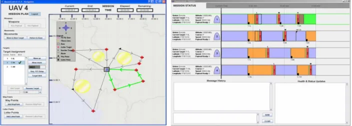
The Multi-Aerial Unmanned Vehicle Experiment (MAUVE) is a computer simulation in which one human operator supervises four UAVs in a time-critical targeting mission. Pre-planned missions are presented to the operator to be executed in real-time. Operator mission tasks during the simulation include arming and firing UAV payloads at scheduled times, re-planning UAV paths in response to emergent threats, assigning emergent targets to the most appropriate UAV, and answering questions about the mission from an automated “supervisor” through a datalink “chat” messaging window. MAUVE consists of a map and decision support display as seen in Figure 1. In addition to the geo-spatial representation, the map display includes a UAV interaction panel which allows operators to send new commands to the UAVs. The decision support display includes a timeline representing all four UAV schedules as well as the chat window for human-human communications and a UAV datalink window for human-UAV communication.
Figure 1: MAUVE map (left) and decision support (right) displays
In the timeline display in the right panel of Figure 1, the different colored bars represent different UAV flight phases. Table 1 shows the color-coding for these different flight phases. A time on target (TOT) is defined as the arming, firing, and battle damage assessment windows on the timeline. Appendix A contains the cognitive task analysis flow charts that depict operator tasking including weapons release, changes in the air tasking order (ATO), and schedule and route replanning.
Table 1: UAV Color-Coded Flight Phases UAV Action Color
Enroute Blue
Loitering Orange
Arming Payload Yellow
Firing Payload Red
Battle Damage Assessment Brown
B. Previous Findings
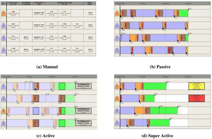
Previous work with the MAUVE simulation involved studying how different levels of automation used within the simulation affected human and system performance (Cummings & Mitchell, in press). Specifically, different automation levels were utilized in depicting timeline. Figure 2 shows the different timeline displays for the manual, passive, active, and super-active automation levels (Cummings & Mitchell, in press). The manual timeline, pictured in Figure 2a, showed scheduled mission events in a tabular format. The passive timeline, as seen in Figure 2b, utilized a graphical color-coded timeline to represent current and future events, but did not provide any indication of high workload areas or decision support. The active timeline, shown in Figure 2c, used a reverse-shading technique to indicate to the user potential high workload periods and provided a recommendation to request a TOT delay for specific targets to mitigate these periods. The final timeline design, super-active, represented UAVs that automatically armed and fired at targets, but allowed the operator to cancel these actions 30 seconds prior to the actual event.
In order to mitigate potential high workloads in all four of the displays, the operator could request a time on target (TOT) delay, to push into the future the target’s TOT, defined as the yellow arming, red firing and brown BDA windows on the timeline. In this manner, operators could manage their schedules and possible future areas of high workload by requesting TOT delays. Requests for a TOT delay were not always granted; the farther into the future a target was, the more likely a TOT delay request for it would be granted. Thus, TOT delay requests made for targets with TOTs close to the present time were rarely granted delays. Additionally, the amount of time a delayed target’s TOT was pushed into the future was not known to the user until the delay was granted. Once the computer determined whether or not the TOT delay request would be granted, it then moved the TOT back so as not to overlap with any other TOTs in the single UAV’s timeline. A granted TOT delay request could, however, create a TOT conflict for the moved target or late target arrivals.
It was predicted that the Active timeline display would produce the best human and system performance since it promoted a collaborative human-automation strategy with the human having the final say, otherwise known as management-by-consent. Specifically, this level of automation highlighted periods of potential high workload to the user, defined as when two or more UAVs had arming, firing or battle damage assessment (BDA) periods scheduled at the same time. These periods are called TOT conflicts and were highlighted through a reverse shading technique, as seen in Figure 2c.
Experiments performed with the four timeline designs unexpectedly determined that human subjects using the active level in the time-critical targeting task performed the worst out of all other levels. Figure 3a shows the performance scores for all four timeline decision support levels under two different levels of mission re-planning.
Figure 2: The four possible levels of timeline decision support in MAUVE (Cummings & Mitchell, in press)
Figure 3: Performance Score & TOT Request Results (Cummings & Mitchell, in press) (a) Manual (b) Passive
(c) Active (d) Super Active
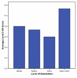
In the low re-planning level, performance scores for all levels of decision support generally were no different. However, in the high level of re-planning, subjects using the active decision support performed significantly worse than subjects using other kinds of decision support (Cummings & Mitchell, in press). This result was traced to the operator’s misuse of the TOT delay request, which should have been used judiciously to eliminate TOT conflicts and late arrivals to targets, but was over-used in the Active display. It was determined that operators using the active level in a high re-planning mission requested significantly more TOT delays than the other levels of decision support, as seen in Figure 3b. Participants under these conditions were unable to generate stopping rules when trying to achieve a particular schedule change. They instead tended to focus more on globally optimizing their schedule and less on performing present mission-critical tasks, such as arming and firing at targets. This caused a reduction in their performance and in their awareness of the current mission situation, as seen in their lower level 2 situation awareness scores, shown in Figure 4 (Cummings & Mitchell, in press).
Figure 4: Level 2 SA Results
Due to these results and previous research that demonstrated that management-by-consent automation strategies were generally the most effective in promoting effective human-automation interaction, it was determined that the active level needed to be redesigned in two ways. First, operators needed an explicit visual representation of the likelihood of a granted TOT delay request in order to generate more effective stopping rules when trying to implement schedule changes. Second, operators needed a tool to better understand the effects of their decisions on both current and future mission schedules.
The attempt to address the second problem of decision propagation representation constitutes the remainder of this report. The first problem was addressed in all displays through the addition of a qualitative probabilistic display for TOT delay request likelihood. Depending upon how far into the future a target was in a UAV’s schedule, the probability bar, depicted in Figure 5, displayed the likelihood of a TOT delay request being granted. Targets located scheduled in the first five minutes were given a low probability of being delayed, those between five and ten minutes had a medium probability, and targets occurring between ten and fifteen minutes had a high probability of being granted a request. This bar was positioned above the TOT Delay Request button so as to
and thus generate better stopping rules when trying to achieve a particular delay or solve a specific schedule problem.
Figure 5: TOT delay request probability bar on mission planning toolbar
III. The StarVis Configural Display and Decision Support Design Implementation A. Initial Analysis and Influence Diagram
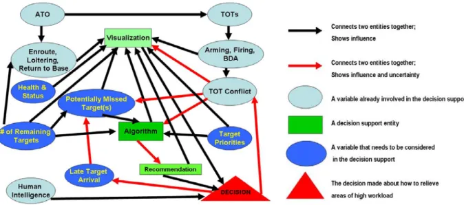
Initial analysis for the MAUVE Active level decision support redesign began with the creation of an influence diagram. An influence diagram maps how variables in a system influence one another. The influence diagram was created to understand what and how variables would influence an operator’s attempts to mitigate high workload mitigation within a mission, and also how the MAUVE system impacted this process. The influence diagram includes the different decision support components, existing variables considered in the previous version of MAUVE, as well as variables that are not yet considered in the decision support design. Figure 6 shows the influence diagram and the associated legend. The focus of this reported research effort was to identify those variables that were critical in terms of supporting the human decision maker through the visualization. The planned second phase of this project is to assimilate this data in an improved intelligent decision support tool that could make recommendations for workload mitigation (as seen in the algorithm and recommendation green blocks in Figure 6).
TOT Delay Request Probability Bar
TOT Delay Request Button
Figure 6: MAUVE schedule management influence diagram
From the influence diagram, it was determined that two problems requiring schedule management occurred within the mission schedule. The first type of schedule problem, called a TOT conflict, indicates a potential high workload area when an operator may possibly be too busy to arm and fire upon multiple targets in a small time period, particularly if they are performing any other mission tasks, such as path re-planning. As discussed previously, potentially moving one of the TOTs in conflict could mitigate operator workload.
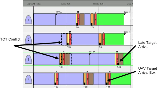
In contrast to the visualization in Figure 2c, TOT conflicts are now indicated on the timeline with dashed boxes around the targets involved in the conflict, as seen in Figure 7. This was a redesign from the original active level of decision support, which placed dashed boxes across all four UAVs when TOT conflicts occurred, and also used a reverse shading technique to further highlight high workload areas. From a human-in-the-loop simulation, it was thought that this original potential high workload notification scheme was too salient and distracted the user from other mission tasks. Thus, the reverse shading technique was eliminated and dashed boxes only surrounded the targets involved in the TOT conflict.
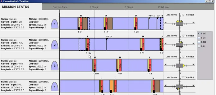
The second problem uncovered in the creation of the influence diagram (Figure 6) is called a Late Arrival (LA). The arrival of a UAV to a target is indicated on the timeline by a small black box labeled with the target’s designation, as seen in Figure 7. If a UAV arrives at a target before the scheduled TOT, it loiters over the target. A LA occurs when a UAV arrives to a target after its scheduled TOT, or if there isn’t enough time left in the TOT for the arming and firing sequence which can take anywhere from 6 to 14 seconds. A target arrival box located after or near the end of the target’s TOT indicates a late arrival. Figure 7 shows a LA for UAV 3 on target T-10H; in this case, UAV 3 is late to T-10H because there isn’t enough time within the TOT to arm and fire upon the target, even though the UAV reaches the target within the scheduled TOT.
Figure 7: Example active level timeline with late arrival and TOT conflict schedule issues
In addition to determining the two schedule management problems, the influence diagram also uncovered additional variables that affected the schedule management, but were not explicitly addressed in the previous version of MAUVE. These variables include the temporal location of the schedule problems within the future timeline and the priority of the targets involved. All of these variables were considered in the redesign of the schedule management decision support.
B. StarVis Design
From the influence diagram analysis as well as results from the previous experiment, the StarVis decision support display was designed. The StarVis design is a configural display integrating many pieces of information about an individual UAV’s potential schedule problems. A configural display is a single geometrical form that maps multiple variables onto it and changes in the individual variables cause the form to vary (Bennett, 1992). The variables represented in StarVis include the type of schedule problem (late arrival or TOT conflict), the number of targets involved in a specific problem type, and their relative priorities (low, medium, or high). Additionally, the StarVis is a projective, “what if” tool allowing operators to see the effects of schedule management decision options projected across the 15 minute timeline. Each UAV timeline in MAUVE has its own StarVis.
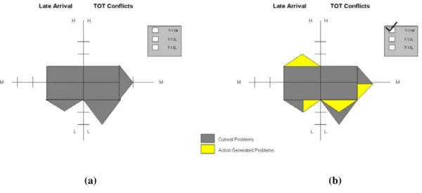
Late Target Arrival TOT Conflict
UAV Target Arrival Box
Figure 8: The StarVis decision support display for MAUVE schedule management
Figure 8 shows the StarVis decision support display for operator management of the MAUVE mission schedule. The StarVis operates in two modes: current and projected problems. Figure 8a shows the default, current problems mode, in which the StarVis shows the schedule problems that currently exist on a UAV’s timeline for the next fifteen minutes. The left side of the StarVis represents targets with late arrivals (LAs). The StarVis’s right side represents targets belonging to the UAV involved in TOT conflicts. If no problems exist in the next fifteen minutes of a UAV’s schedule, the StarVis simply contains a gray rectangle. Gray triangles begin to grow off a UAV’s StarVis when problems are detected. Targets of high priority involved in schedule problems are represented by triangles that emerge from the top of the triangle. Targets of medium and low priority are represented by triangles on the sides and bottom of the rectangle, respectively. The height of the triangles gives the number of targets involved in a particular problem with a specific priority. In the example given in Figure 8a, the StarVis shows that for its UAV’s schedule, there is one low priority target expected to be late, one medium priority and two low priority targets involved in separate TOT conflicts with targets from other UAVs.
Next to the StarVis is a list of targets that have schedule problems on the UAV’s timeline and are represented by one or more triangles on the StarVis. By selecting one of the checkboxes, the operator puts the StarVis into a projective mode, as shown in Figure 8b. By selecting a checkbox, the operator is virtually querying “if I request a TOT delay on this target, and it is granted, what will happen to my individual UAV’s schedule?” Selecting a checkbox may cause yellow triangles to appear, which represent how the schedule would change if the TOT request is made. Split gray and yellow triangles indicate that the same problem that exists on the current timeline would continue to exist if the selected target was delayed. Gray triangles continue to indicate current timeline problems. For the example shown in Figure 8b, if a TOT delay request for target T-11M is granted, the UAV will still have a low priority target late arrival and a medium priority target involved in a TOT conflict, problems that exist on the current timeline. Additionally, there will be one less low priority target involved in a TOT conflict, and the addition of a high priority target late arrival.
The StarVis was designed in order to leverage direct perception-action which allows operators the ability to utilize more efficient perceptual processes rather than cognitively demanding processes that rely on memory, integration, and inference (Gibson, 1979). The efficient and effortless power of perception make utilizing direct perception-action an important principle in the design of user displays, and has been shown to improve operator performance in complex tasks (Buttigieg & Sanderson, 1991; Sanderson, 1989) In addition, the StarVis was designed to support the proximity compatibility principle (Wickens & Carswell, 1995) through integration of those variables that operators need for some kind of comparison or computation (either arithmetic and/or Boolean), identified from the previously described influence diagram (Figure 6). For example, the StarVis allows operators to easily determine the number of targets predicted to be future problems for one UAV and then easily compare this number with another UAV to determine if a particular course of action is warranted.
One important feature of configural displays that exploit the benefits of direct perception is the concept of an emergent feature. Emergent features are produced by the interaction between display elements, thus variables, and provide a higher-level aggregate view of a system state (Bennett, 1992). In MAUVE, as a mission plan begins to experience problems, either through later arrivals or TOT conflicts, visual representations of these problems “emerge” as spikes grow from either side. In a quick glance, operators can immediately discern for not just one UAV, but for all of them, whether or not any problems exist (no spikes = no problems), and in general the surface area provides for direct comparison as to which UAV is experiencing the most problems, and specifically what kind. Thus the StarVis provides a high-level overview through emergent features, but also provides low level details should an operator decide to focus on a particular variable of interest.
The StarVis’s dual representation of a high level overview and low level detail is critical for command and control applications where rules of engagement (ROE) are dynamic. ROE can change in the course of months, days, and even hours, and thus a robust decision support tool is one that can support operator decision making under these dynamic conditions. For example in StarVis, if operators determine that they really only are concerned with ensuring no high priority late arrivals occur, they then can essentially focus on the right upper quadrant and make decisions accordingly.
C. StarVis Implementation
Once the configural StarVis decision support display was designed, it was implemented into the MAUVE simulation in two different decision support visualization designs. Two different StarVis decision support visualizations (DSVs) were designed: A Local StarVis DSV and a Quasi-Global (Q-Global) StarVis DSV. Both StarVis DSV designs visualize current timeline problems through gray triangles in the same manner; the designs differ in the way the projective “what if” mode shows the affects of decisions on the DSV after the user selects target checkboxes.
1. Local StarVis DSV
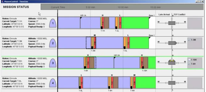
Figure 9 shows the Local StarVis DSV design, which will be referred to as the Local StarVis. As previously stated, each UAV has its own StarVis configural display, which allows for overall comparison. Next to each StarVis is a list of targets that have problems for that UAV’s current schedule and are represented on the StarVis with gray triangles. The operator may select only one target checkbox for each UAV’s StarVis in order to activate the projective “what if” mode. However, multiple UAV StarVis displays can have checkboxes selected. Figure 10 shows an example of a Local StarVis with both the checkboxes unchecked and checked.
Figure 9: Timeline display with Local StarVis decision support visualization.
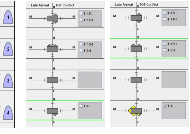
In Figure 10a, the UAV has a single TOT conflict for a low priority target, which is identified as target T-4L in the list to the right of the StarVis. Figure 10b shows the StarVis with the checkbox selected for T-4L. By selecting this checkbox in the Local StarVis design, the operator is virtually asking, “If I request a TOT delay for UAV 4’s target T-4L and it is granted, what will happen to UAV 4’s schedule?” Once clicked, yellow triangles appear showing the “what if” condition for UAV 4 only. Selecting a target checkbox for a UAV shows what would happen to only that UAV’s schedule if that target is delayed. In Local StarVis, yellow triangles can only possibly appear on the other UAV StarVis displays if target checkboxes belonging to those UAVs are selected. Each UAV StarVis may only have one target checkbox selected at a time, but multiple UAVs may have a target checkbox selected. This allows for the comparison of decision alternatives when attempting resolving schedule problems such as TOT conflicts, which involve multiple targets belonging to different UAVs.
Figure 10: Local StarVis DSV: (a) current timeline problem and (b) current timeline problems with a “what if” projection
2. Quasi-Global StarVis DSV
Figure 11 shows the Quasi-Global StarVis DSV, which will be referred to as the Q-Global StarVis. This StarVis decision support visualization is quasi-global because it allows a user to explore the consequences of different individual problem decision options upon all the UAV schedules and allows for layering schedule management decisions. The Q-Global StarVis, however, does not inform the user how to fix all timeline problems at once. The Q-Global StarVis DSV design was created in response to the Local StarVis’s incapacity to show the potential affects of schedule management decisions across all UAVs. As with the Local StarVis design, each UAV has its own StarVis configural display in the Q-Global StarVis DSV.
As seen in Figure 11, the Q-Global StarVis lists all targets that have current timeline problems together, instead of separating them for their respective UAVs. If no target checkboxes are selected, the information displayed on the Q-Global StarVis DSV is exactly the same as the information displayed on the Local StarVis DSV. The two DSV designs differ when checkboxes are selected and the “what if” tool is engaged.
Figure 12 shows an example of the Q-Global StarVis with checkboxes unchecked and checked. In the Q-Global design, multiple checkboxes may be selected. If one or more checkboxes are selected, the operator is virtually querying “If I request a TOT delay for the selected target(s) and the delay(s) is granted, what will happen to ALL UAV schedules?” Yellow triangles may appear on all the UAV StarVis configural displays, but not necessarily. Split triangles on a UAV’s
StarVis configural display indicate that a specific problem that exists on the current schedule for the UAV will exist if the selected targets are granted a TOT delay. Purely yellow triangles indicate that new problems will arise if the selected targets are delayed.
Figure 11: Timeline display with Quasi-Global (Q-Global) StarVis decision support visualization.
In contrast to the Local StarVis DSV, the Q-Global StarVis DSV design shows the propagational effects of delaying target TOTs on all the UAV schedules, instead of only the UAV schedule that the target is assigned to. Additionally, with the Q-Global StarVis, multiple targets can be selected in the list of targets involved in problems which allows for the layering of multiple schedule management decision options. However, if the operator selects multiple target checkboxes, he or she needs to consider the order in which decisions are made and implemented, as schedule management decision implementation is not a commutative property. Requesting a delay for target A and then for target B may have a different affect on the schedule than if target B is delayed before target A.
IV. Experimental Protocol
This experiment protocol outlines the objectives, research question, task, independent and dependent variables, and experimental design for human subject testing of the different StarVis decision support visualizations.
A. Experiment Objective
The main objective in this experiment is to determine if decision support visualizations that project possible future states based upon decision alternatives assist humans in making schedule management decisions that optimize human and system performance. Three workload mitigation decision support visualizations were tested: a control visualization that consisted of only a timeline, one that combined the timeline and the StarVis configural display in a Local implementation, and a visualization that utilized the timeline and the Q-Global StarVis decision support visualization.
B. Research Hypotheses
Due to the inability of humans to accurately predict effects of temporal decisions upon a schedule in the face of uncertainty, it was hypothesized that one of the two StarVis decision support visualizations (DSV) would result in better human performance in managing a multiple UAV mission schedule over the timeline only condition. This was hypothesized primarily because of the following benefits of the StarVis configural display:
1. The StarVis configural display offers both a quick overview of any UAV scheduling problems as well as a graphically comprehensive, lower level view of current timeline issues
2. The StarVis display contains a “what if” tool that visualizes the possible effects of decisions if executed
In terms of which StarVis display would be superior, the, benefits and costs of both displays were determined:
1. The Local StarVis allows for multiple decision alternatives to be compared, allowing operators to fully consider the effects of all decision options, leading to optimal decision choices, as seen by a reduction in schedule problems for individual UAV timelines.
However, the Local StarVis also could incur some costs in its usage:
1. Because the effects of decision alternatives displayed on StarVis are only for the UAV involved in the original schedule issue, operators will not fully take into account the effect of decisions upon the whole system and instead will focus on individual UAV optimization. This could lead to increases in schedule problems. 2. With a lack of information about decision repercussions on the whole system,
possible increases in schedule problems could lead to higher operator workload, both objectively and subjectively perceived.
Q-Global StarVis DSV usage has the following potential benefits:
1. The Q-Global StarVis shows the operator the possible effects of a decision upon all the UAVs in the mission. This may give the operator a more system-wide view of the mission, increasing both level 2 and level 3 situation awareness (SA).
2. Because the Q-Global StarVis visualizes how delaying multiple targets affects UAV schedules, this DSV allows combining multiple decisions through decision layering and shows the resultant effects. This may result in increase human performance in mission objective achievement and a reduction in schedule problems across all UAV timelines.
Drawbacks to the Q-Global StarVis DSV include:
1. Because of the inability to compare the alternatives of one decision directly, operators may spend excessive time trying to optimize one decision or a combination of decisions, leading to a lack of situation awareness.
Because these advantages and disadvantages did not convey any clear prediction as to which StarVis implementation would be superior, we treated this as an open research question.
C. Task
In this MAUVE simulation experiment, the operator’s main task was to supervise four UAVs in a time-critical targeting mission. Specifically, the operator needed to:
1. Guide each individual UAV’s actions so that all UAVs properly executed required mission commands, which changed over time
2. Answer questions about the mission situation through the instant messaging tool Supervision of the entire mission was broken down into prioritized sub-tasks, listed from highest priority to lowest:
3. Destroy all targets before their time on target (TOT) window ends by manually arming and firing a weapon.
4. Perform battle damage assessment (BDA) on specified targets after destroying them 5. Avoid damage from enemy fire by navigating around and out of threat areas
6. Answer communication questions Operators were explicitly trained to follow this priority list and these prioritized tasks were displayed throughout training and test sessions. In order to perform the mission, the operator was given the two MAUVE displays in Figure 1. All subjects used the same map display, but subjects were given either a timeline only, timeline with Local StarVis, or timeline with Q-Global StarVis display in order to complete their multiple UAV mission management task. In supervising the mission, the operator needed to manage the mission schedule in order to achieve mission objectives. This involved executing the schedule, as well as dealing with schedule problems predicted in the future, such as late arrivals and TOT conflicts. Late arrivals to targets could be solved by either path re-planning, if possible, or by requesting a TOT delay. TOT conflicts could only be mitigated by requesting a TOT delay. In deciding how to solve both of these timeline-related problems, the operator had the option of using the timeline and the StarVis (if provided) to explore different decision alternatives for schedule management.
D. Independent Variables
There were two independent variables in this experiment: 1) Schedule management decision support visualization type and 2) Level of re-planning. Visualization type was a between-subjects variable, and consisted of three different displays: 1) A control display in which a graphical mission schedule was provided, 2) a display with the same graphical timeline schedule plus the experimental Local StarVis decision support visualization, and 3) A display
with a graphical timeline schedule and the Figure 13: The Three Experimental Displays (c) Q-Global StarVis
(a) Timeline Only
experimental Quasi-Global decision support visualization. Figure 13 shows the three possible schedule management decision support visualizations.
The second independent variable, level of re-planning, was a within-subjects variable. It represented the operational tempo of re-planning events, both in the number of events and how they are spaced in a given simulation scenario. It was included since in the previous experiment, level of replanning showed very different patterns for operator performance. Types of re-planning events included:
• Emergent targets needed to be added to the mission timeline • Assigning a target to a different UAV strike mission
• A new threat area appeared in the navigation display • A threat area became inactive
• Battle damage assessment needed to be added to an existing target’s schedule • Battle damage assessment needed to be removed from an existing target’s schedule • A UAV was commanded to return to base during the mission
Each subject was exposed to the two re-planning levels. A low re-planning level contained 7 events, spaced by approximately 3 minute intervals, with each interval containing only one event. A high re-planning level contained 13 events, spaced at approximately 3 minute intervals with each interval containing 2-3 events. Subjects underwent training before completing actual experimental mission scenarios. The order in which a subject completed the two test scenarios was randomized in order to control for possible learning effects.
E. Dependent Variables
Multiple human and system performance dependent variables were measured in this experiment. They included two different performance scores, number of TOT delay requests, secondary workload, subjective workload, late arrival and TOT conflict mitigation scores, number of critical firing events, and a situation awareness measure.
1. Optimistic Performance Score
This score, developed for the previous experiment (Mitchell, 2005) was designed to be an overall measure of test session performance. This metric relates to the experiment’s research question, as the goal of the StarVis decision support visualizations was to assist the operator in understanding decision alternatives so as to achieve mission objectives. A subject’s performance score was based upon the total number and type of mission objectives completed over an entire testing session, with penalties applied for actions resulting in negative consequences for the mission plan. Thus, this score had earned points (positive) and penalty points (negative). A higher score indicated better performance in a test session.
a. Earned Points
An operator earned points by destroying targets on time or correctly performing BDA. The base number of points earned for achieving an objective (either correctly destroying a target or correctly performing BDA) corresponded to the allotted time it took to perform the objective. Table 2 shows the number of base points awarded for objective achievement.
Table 2: Base points for performing mission objectives (Mitchell, 2005)
Event Base Points
Target Correctly Destroyed 30
BDA Correctly Performed 45
Taking into account target priority and target difficulty further modified target scores. Target priority refers to the low, medium, and high modifiers assigned to each target. Target difficulty refers to how difficult it was to destroy a target due to re-planning, the number of simultaneous events near or during the target’s TOT, and where in the timeline (start, middle, or end), the target was scheduled. Each target was assigned a difficulty of low, medium, or hard based upon these factors, as well as upon previous experimental data on how often operators missed that target. Table 3 shows the modified target scores for different combinations of target priorities and difficulties.
Table 3: Modified target scores for different combinations of target priorities and difficulties (Mitchell, 2005)
Priority Difficulty Modified Target score
High Hard Medium Low 67.5 60 52.5 Medium Hard Medium Low 52.5 45 37.5 Low Hard Medium Low 37.5 30 22.5
BDA scores were further modified only by difficulty, with two classifications of difficult or easy based upon whether or not the BDA event was affected by re-planning. BDA that was scheduled by the operator as a mission re-plan was considered difficult, while BDA that was initially scheduled before the mission scenario began was dictated as easy. Table 4 shows the modified BDA scores awarded for correctly performed BDA
Table 4: Modified BDA score based upon difficulty (Mitchell, 2005)
BDA Difficulty Modified BDA Score
Difficult 45 Easy 22.5
b. Penalty Points
Penalty points were deducted from the performance score if the operator destroyed a target when previously commanded not to, incorrectly performed BDA, had a UAV fired upon in a threat area, or arrived at base past the mission time limit. Table 5 shows the values of penalty points associated with actions that deter mission objectives.
Table 5: Penalty points associated with actions deterring mission objectives (Mitchell, 2005)
Event Penalty Points
Target Incorrectly Destroyed 45
BDA Incorrectly Performed 0
Hit in Threat Area 10
Late Arrival to Base 1 per second per UAV
For incorrectly destroyed targets, the penalty deduction value was chosen to be the average score of a correctly destroyed target (45 points). For incorrectly performed BDA, no penalty was deducted because it was assumed that the wasted time spent performing that BDA would cause time penalties in future events (Mitchell, 2005).
2. Pessimistic Performance Score - Performance Score with TOT Delay Penalty
Although requesting a TOT delay is a mission schedule management option that can result in higher human and system performance, operators sometimes tend to make excessive requests and thus abuse the TOT delay request function (which was seen in the previous experiment). This behavior would have tangible consequences in actual military operations, where excessive requests can cause negative repercussions in organizations beyond decreases in an individual operator’s performance such as saturation of communication lines and wasting of resources. Thus, a second performance score was created in order to reflect abuse of this function. It deducted from the optimistic performance score one point per each second the time the request took. Five seconds were required to receive a response from a TOT delay request; thus 5 points were deducted from a subject’s optimistic performance score for each TOT delay request made, regardless of whether or not the request was granted.
3. Number of TOT Delay Requests
The number of TOT delay requests was measured in order to verify if a correlation between performance and the number of TOT delay requests existed. Previous work, as discussed earlier in this report, found that in the active level of decision support, performance was lower and the number of TOT delay requests was higher when compared to the other decision support levels (Cummings & Mitchell, in press). The number of TOT delay requests can also be compared with situation awareness and workload measures to ascertain if requesting TOT delays positively or negatively affects other aspects of human interaction with the system. This metric was simply a count of the number of TOT delay requests an operator made in each test scenario.
4. Secondary Workload
Workload measures were relevant to this experiment as the main goal of the workload mitigation decision support visualization was to reduce the number and duration of high workload periods in a mission schedule. Secondary workload was measured by the length of response times to the online chat questions that appeared at predetermined times in each experimental mission scenario. Previous research showed that chat question responses is an effective technique for measuring spare mental capacity, and thus workload, in command and control settings (Cummings & Guerlain, 2004). The response lengths to questions were added together and averaged over the total number of questions asked. In the case of an operator not answering a chat question, the duration of response length was taken as the time between when the question was asked to when the next chat question was asked. The assumption that chat questions go unanswered because the operator is experiencing high workload is valid, as answering communications was ranked as the lowest operator task in the mission objectives priority list.
5. Subjective Workload
In addition to reducing actual workload, the addition of a workload mitigation decision support visualization should not increase perceived operator workload. Thus a subjective workload measure was determined using the NASA Task Load Index (TLX) subjective workload rating survey. The survey computed a workload score from operator-weighted ratings on a 1-20 scale along six dimensions, which included mental demand, physical demand, temporal demand, effort, performance, and frustration (Hart, 1988). Because the mission task involved no physical demand, subjects were told to purposefully rank physical demand as a low contributor to workload and ignore survey portions asking about that dimension. Thus the survey was modified to be based upon the other five dimensions and minimized physical demand as a workload contributor in the multiple UAV command and control task.
6. Late Arrival Mitigation Score
The late arrival mitigation score documented the number of late target arrivals the operator either eliminated or generated within a mission scenario. As decreasing the number of late target arrivals increases the number of possible targets an operator may destroy to improve their performance score, measuring late arrival mitigation was relevant to the experiment. Each time a late target arrival was generated, either through the scenario or through operator attempted schedule management, a point was deducted from the score. However, each time an operator eliminated a late target arrival through proactive schedule management, a point was added. Good performance in late arrival mitigation was indicated by a high score. The highest a subject could receive was a score of 0, indicating that all late arrivals were mitigated. Thus, the more negative a late arrival mitigation score was, the less the subject was able to mitigate late target arrivals.
7. TOT Conflict Mitigation Score
Similar to the late arrival mitigation score, the TOT conflict mitigation score measured the number of TOT conflicts the operator either eliminated or generated within a mission scenario.
This metric related to the research question as the goal of a schedule management decision support tool is to assist the operator in managing his schedule by reducing the number of high workload areas, so as to decrease operator workload and possibly increase performance. Each time a TOT conflict was created, either through the scenario or through attempted schedule management, a point was deducted from the score. However, each time the operator eliminated a TOT conflict a point was added. Good performance in this area was indicated by a high score. As with the late arrival mitigation score, the highest score a subject could receive was a score of 0, and the more negative a TOT conflict mitigation score was, the less the subject attempted to eliminate TOT conflicts.
8. Number of Critical Firing Events
The number of critical firing events documented the number of times an operator fired upon targets that previously were specified not to be destroyed. This score was used as an overall global situation awareness measure. The command not to fire upon specific targets was given within mission scenarios as a re-planning event with an associated message. The number of critical firing events was summed for all operators within a given decision support visualization assignment, and thus reflected a total across all subjects as opposed to scores for individual subjects. This metric was relevant to the research question as it indicated an important measure of overall situation awareness that signified a critical measure in real-life UAV applications. As with other situation awareness measures, it was important that the decision support system assist in facilitating rather than detracting from operator situation awareness.
9. Situation Awareness
A measure of situation awareness (SA) combining level 2 and level 3 SA was adapted for this experiment based on previous measures (Mitchell, Cummings, & Sheridan, 2005). Four indicators of situation awareness determined from mission scenarios were:
1. The number of entries into threat areas where the UAV received more than 3 hits and the operator did not take any action to minimize further damage to the UAV.
2. The amount of time UAVs loitered at missed targets due to loss of situation awareness 3. The number of targets missed due to lack of situation awareness
4. The percentage of re-planning events successfully and correctly completed.
These four indicators combined represent level 2 (comprehension) and level 3 (future projection) situation awareness (Endsley, 1995). Different ranges of possible values for each of the SA indicators were grouped and then ranked on a 1-5 scale. Table 6 shows the relative 1-5 scale and the relative range of values for each indicator (Mitchell et al., 2005).
Table 6: Situation awareness indicators and relative scales Situation Awareness Score Number of significant entries into threat areas, no operator intervention
Amount of time UAVs spent loitering at missed or removed targets (s) Number of targets missed due to lack of SA Percentage of re-plans successfully completed 5 0 0 - 30 0 -1 90 or more 4 - 30-90 2 - 3 80 - 90 3 1 90-120 4 70 -80 2 - 120-200 5 60 -70
1 2 or more 200 or more 6 or more 60 or less
F. Apparatus, Participants, and Procedure
The experiment, including training and testing, was performed on a four screen system called the multi-modal workstation (MMWS), shown in Figure 14.
Figure 14: The Multi-Modal Workstation (MMWS)
The top three 21 in. screens were run at 1280 x 1024 pixels, 16-bit color resolution, while the 15 in. bottom screen was run at 1024 x 768 pixels, 32-bit color resolution. The workstation computer was a Dell Optiplex GX280 with a Pentium 4 processor and an Appian Jeronimo Pro 4-Port graphics card. Experimental subjects interacted with the MAUVE simulation through a generic corded mouse and cordless keyboard. The top leftmost screen contained a listing of the mission objectives in priority order for the scenarios and was static throughout the entire experiment. The top middle screen contained the MAUVE map display and the top rightmost screen contained a MAUVE timeline/decision support display. During testing, all mouse clicks and all message box histories were recorded by the MAUVE software. In addition, screen recording of both the map and timeline/decision support displays was performed by Camtasia® screen capture recording software.
A total of 15 participants, 11 males and 4 females, took part in this experiment. The subject population consisted of students, both undergraduates and graduates, and young professionals in technical fields. All subjects were paid $10 per hour for their participation, and a $50 gift certificate was offered as an incentive prize to the best performer in the experiment. The age range of subjects was 20 to 31 years, with an average age of 24 years. None of the participants had any military experience.
The format of the experiment consists of three distinct phases: Training scenarios, experiment scenarios, and post-experiment feedback. In the training phase, all subjects received between 90 and 120 minutes of training over three to four practice scenarios until they demonstrated basic competency in use of the MAUVE simulation and mission objectives. Practice scenarios were presented to subjects in the same format and order. The first scenario familiarized subjects with the basic displays, mission execution actions, and rules of engagement, while the second scenario introduced all possible re-planning events. The third scenario consisted of a hands-off 15 minute test similar to the experimental mission scenarios, including previously unseen chat questions about the mission. After the third scenario, additional practice could be given if needed in a fourth scenario unique from the previous three.
If the subject demonstrated proficiency in training, he or she was then tested on two consecutive 30 minute mission scenarios, one each of low and high mission re-planning levels. Each of these scenarios represents a pre-planned mission that a separate agency developed, which is typical of military operations. The order in which the subject was exposed to the low and high re-planning levels was randomized and counter-balanced. All subjects saw the same scenarios, the only difference being the type of schedule management decision support visualization they were exposed to in the decision support display. After each mission scenario, the subject completed a NASA TLX survey. After all experiment mission scenarios were completed, subjects were asked to fill out a post-experiment feedback questionnaire which asked for their thoughts on the MAUVE interface as well as on the schedule management decision support.
V. Results
For statistical analysis of the experimental data, a 2x2 repeated measures MANOVA was used, which considered both re-planning level (low vs. high) and decision support visualization type (no visualization (NV), Local StarVis (LV), and Global StarVis (GV)). In addition, Pearson Correlations were found in order to determine relevant relationships. Box plots of the dependent variables for the different experimental conditions were also made in order to gain more understanding about the range, variance, and means of the dependent variables.
A. Performance Scores using Repeated Measures MANOVA
A summary of the statistical results using repeated measures MANOVA is given in Table 7. For reference, p values less than 0.05 are statistically significant, while p values between 0.05 and 0.1 are marginally significant. The results should be evaluated in light of the somewhat small sample size, N=15, however a repeated measures design was employed in order to reduce error
Table 7: Summary of experiment statistical results.
Dependent Variable
Level of Replanning
Visualization Interaction Tukey p values for the Visualization Factor NV-LV NV-GV LV-GV Optimistic Performance F(1,12)=27.3 p<.001 F(2,12)=9.3 p=.004 NS .028 .482 .003 Pessimistic Performance F(1,12)=22.5 p<.001 F(2,12)=9.9 P=.003 NS .009 .903 .004 # TOT delay Requests F(1,12)=4.1 p=.065 NS F(2,12)=3.8 p=.053 - - - Secondary Workload F(1,12)=7.1 p=.02 NS NS - - - Subjective Workload F(1,12)=4.1 p=.065 F(2,12)=3.8 p=.052 NS .142 .834 .052 Situation Awareness F(1,12)=45.9 p<.001 F(2,12)=9.8 p=.003 F(2,12)=5.7 p=.018 .004 .775 .013
1. Optimistic Performance Score Figure 15 shows box plots for the optimistic performance score for the three visualization conditions under the two different levels of planning. Both the level of re-planning (F(1,12)=27.3, p<.001) and visualization type (F(2,12)=9.3, p=.004) were statistically significant. Tukey post-hoc comparisons demonstrate that subjects with the Q-Global StarVis performed statistically no different as those subjects with no visualization (p=.482) while those with the Local StarVis outperformed both Q-Global (p=.003) and those with no visualization (p=.028). One interesting trend to note is that those performance scores for subjects assigned to any StarVis condition tended to have less variation than performance scores from subjects in the no visualization condition.
Low Re-planning High Re-planning
Re-Planning Level 200.0 300.0 400.0 500.0 600.0 700.0 800.0 900.0
Optimistic Performance Score
13 17 17 Visualization Type No Visualization Local StarVis Q-Global StarVis
2. Pessimistic Performance Score The statistical analysis of pessimistic performance yielded a similar result to the optimistic performance scores. Again, both the level of re-planning (F(1,12)=22.5, p<.001) and visualization type (F(2,12)=9.9, p=.003) were statistically significant in this measure. Figure 16 shows the box plot for the pessimistic performance score, which as previously discussed, differed from the optimistic performance score by penalizing subjects every time they requested a TOT delay, regardless of it being granted. As with the optimistic performance score, subjects using the Local StarVis decision support performed better than subjects in the no visualization and Q-Global StarVis conditions. Tukey post-hoc comparisons also exhibited the same pattern as did the optimistic performance score in that subjects with the Q-Global StarVis performed statistically no different as those subjects with no visualization (p=.903) while those with the Local StarVis outperformed both Q-Global (p=.004) and those with no
visualization (p=.009). Furthermore, subjects with either
StarVis decision support designs again tended to have more consistent performance than subjects with the timeline only.
Figure 16: Box plot of Pessimistic Performance Score
Low Re-planning High Re-planning
Re-Planning Level 200.0 400.0 600.0 800.0 Pe ssimis tic Pe rfor ma nce S c o re 1 13 17 17 Visualization Type No Visualization Local StarVis Q-Global StarVis
Figure 17: Interaction for Number of TOT Delay Requests
Low High Re-Planning Level 10 15 20 25 Estimated Marginal Means Visualization Type No Visualization Local StarVis Q-Global StarVis
3. Number of TOT Delay Requests While only marginally significant for re-planning level (F(1,12)=4.1, p=.065), the number of TOT delays also demonstrated a marginally significant interaction (F(2,12)=3.8 p=.053). Figure 17 demonstrates that for both StarVis displays, as the level of replanning increased, subjects responded with increased TOT requests, while those with no visualization decreased their TOT requests as their objective workload increased. Thus, in general, a decision support visualization for schedule management helped operators see current timeline issues. 4. Secondary Workload
Secondary workload was expectedly statistically significant across level of re-planning (F(1,12) = 7.1, p=.02), but was not significant across visualization type, as can be seen by the box plot of the different experimental conditions in Figure 18. It was expected that secondary workload would be statistically significant cross re-planning level, as the different re-planning levels represented different operational tempos which would affect the workload experienced by the experimental subjects. However, the fact that secondary workload did not increase statistically with the addition of any StarVis DSV is a promising result since the StarVis did not add any additional workload for the operator.
Figure 18: Box plot of Secondary Workload
Low Re-planning High Re-planning
Re-Planning Level 12:00:15.000 12:00:30.000 12:00:45.000 12:01:00.000 12:01:15.000 Se co nda ry Wor k loa d 11 2 Visualization Type No Visualization Local StarVis Q-Global StarVis
Low Re-planning High Re-planning
Re-Planning Level 30.0000 40.0000 50.0000 60.0000 70.0000 80.0000 90.0000 S u b jec ti ve W o rk lo a d 2 12 4 17 Visualization Type No Visualization Local StarVis Q-Global StarVis
5. Subjective Workload
Subjective workload was marginally significant in both re-planning level (F(1,12)=4.1, p=.065) and visualization type (F(2,12)=3.8, p=.052). However, as seen by the associated box plot, shown in Figure 19, subjects with Local StarVis subjectively experienced less workload, particularly for the high re-planning condition. Statistically, the subjective workload for those with Local StarVis was no different across low and high replanning.
6. Number of Critical Firing Events
The number of critical firing events measured global situation awareness for all subjects in each visualization condition. A Chi Square test was used to statistically analyze the experimental results, and although not significant across the visualizations, the trend for critical firing events in each visualization condition was in favor of the Local StarVis. Figure 20 shows the total number of critical firing events for all subjects combined in each visualization condition.
Not one critical firing event occurred with any subjects in the Local StarVis decision support. The number of critical firing events with the Q-Global decision support actually exceeded that of subjects with no visualization, showing a decrease in global situation awareness with use of the Q-Global StarVis DSV.
Figure 20: Number of total critical firing events for each visualization condition
Critical Events 0 0.5 1 1.5 2 2.5 3 3.5
No Vis Local Q-Global
# of Events
7. Situation Awareness
The situation awareness (SA) measure, as described previously, was statistically significant across levels of re-planning (F(1,12)=45.9, p<.001) and visualization type (F(2,12)=9.8, p=.003). Tukey post-hoc comparisons demonstrate that subjects with the Q-Global StarVis had no difference in situation awareness as those subjects with no visualization (p=.775) while those with the Local StarVis had superior SA as compared to both Q-Global (p=.013) and those with no visualization (p=.004). Thus the Local StarVis enabled operators to be more aware of their current and projective future states.
Figure 21 shows the box plots for subject situation awareness for all
visualization types across the different re-planning levels. The results for the high re-planning level are particularly revealing in that subjects with the Local StarVis decision support had significantly better awareness of the mission situation, both in the present and future projective sense, than other subjects. Even more interesting, while there was a large drop in situation awareness in the no visualization and Q-Global StarVis conditions as the level of replanning increased, the Local StarVis produced statistically identical performance across the increase in objective workload. Thus the Local StarVis allowed subjects to maintain high levels of SA, even while their workload essentially doubled. Clearly this kind of robustness to large increases in workload is a useful design consideration.
B. Correlations
In order to gain more insight into the experimental data, Pearson Correlations were calculated to examine relationships in the data sets, particularly to examine how different variables influenced subjects’ overall performance. Since we measured two performance scores, we elected to only use the pessimistic performance score in these correlations since optimistic and pessimistic were highly correlated (r = .953, p < .001), and the pessimistic performance score represented the worst case for a subject.
Low Re-planning High Re-planning
Re-Planning Level 2.5 3 3.5 4 4.5 5 To ta l SA 1 6 Visualization Type No Visualization Local StarVis Q-Global StarVis
The number of TOT delay requests negatively correlated with performance (r = -.550, p =.002). This was expected, as previous research demonstrated that subjects that performed poorly tended to request more TOT delays than subjects with better performance (Cummings & Mitchell, in press). Across the different visualizations, the TOT Delay requests correlations are as follows:
• Timeline Only (No StarVis) r =-.355, p=.315 • Local StarVis r =-.523, p=.121 • Q-Global StarVis r =-.789, p=.007
Thus those subjects with the Q-Global visualization demonstrated significantly worse performance as the umber of TOT Delay Requests increased.
Subjective workload also negatively correlated with pessimistic performance (r = -.487, p = .005), meaning that subjects who did well did not perceive their workload to be excessively high. Situation awareness strongly correlated with performance (r =.828, p < .001), and as would be expected, the best performers clearly had the highest awareness about their current and projective future situation.
While these previous correlations were generally expected, more interesting and unexpected results emerged when late arrival and TOT conflict mitigation scores were correlated with performance scores. Late arrival mitigation was correlated with performance (r = .553, p=.002), meaning that one of the ways the best performers achieved their higher scores was through mitigating late arrivals. The late arrival mitigation correlation to performance was also broken out across the different visualizations, with the following results:
• Timeline Only (No StarVis) r =.715, p=.020 • Local StarVis r =.721, p=.019 • Q-Global StarVis r =.102, p=.780
Thus those operators with the Local StarVis and no visualization had better performance scores as a function of late arrival mitigation, which did not show any relationship with the Q-Global visualization.
TOT conflict mitigation was negatively correlated with performance (r = -.366, p =.047). This negative correlation is consistent with the results from the TOT Delay Request MANOVA results. The best performers tended to mitigate fewer TOT conflicts. Thus, they weighted late arrivals as a more important problem than TOT conflicts.
VI. Discussion
The experiment yielded many interesting results pertaining to the use of the configural StarVis display and its Local and Q-Global implementations. The key finding in the experiment was that subjects with the Local StarVis decision support performed better on a number of metrics than subjects with the Q-Global StarVis DSV or no DSV at all. Local StarVis achieved better overall performance scores, requested fewer TOT delays, experienced lower subjective workload, and
that the Local StarVis subjects did better than the Q-Global StarVis subjects, yet both sets of subjects used the same configural StarVis display, but in a slightly different context.
We expected that the Local StarVis subjects would outperform the subjects with no visualization since they had access to an information aggregation tool, but the large gap in performance and other metrics was not expected between the Local StarVis and Q-Global StarVis DSVs. Across almost every metric, those subjects with Q-Global performed at the same degraded level as those subjects with no visualization. Thus one configural decision support tool, applied in two slightly different contexts, contributed to either very good or poor performance. We hypothesize that this disparity in performance between the two StarVis conditions could be due to the fact that Q-Global StarVis subjects were possibly given too much information, especially is they used the projective “what if” tool.
Because of the design of the Q-Global and the composition of the mission scenarios, selecting a target checkbox often caused many split triangles (showing current and projective problems) and yellow triangles (showing projective problems) to appear on one or more StarVis configural displays. Thus, operators had difficulty quickly understanding if delaying the selected target(s) was a good decision because they had to look at potentially all the UAV StarVis displays. In the Local StarVis design, however, selecting one target checkbox only affected the StarVis display on one UAV. Thus, Local StarVis operators needed to only look at StarVis displays that corresponded to the checkboxes they had selected. This resulted in operators having less information to analyze in the “what if” condition. Although the Local StarVis was limited as compared to the full information provided in the Q-Global StarVis condition across all UAVs, the projective “what if” information given in the Local StarVis was enough to help operators make effective decisions, even though the information was not globally optimal. Thus the Local StarVis display supported a “fast and frugal” heuristic (Todd & Gigerenzer, 2000) which allowed subjects to quickly gather just enough information to make a “good enough” decision (otherwise known as satisficing (Simon et al., 1986)). Such “just-in-time decision support” tools are particularly useful in dynamic, military command and control environments where time pressure and uncertainty are high.
Additionally, the Local StarVis design tended to be more intuitive to users as it allowed for multiple decision options to be considered at the same time. This was particularly true for TOT conflicts, where users could select the projective checkboxes for the targets involved and compare the effects directly on the individual timeline. Users using the Q-Global StarVis tended to have more difficultly in comparing the effects of delaying one target on the schedule versus taking no action. Toggling behavior, where users selected and deselected one target checkbox multiple times, was a strategy used by Q-Global StarVis subjects to try to understand the difference in the current schedule and the what-if schedule for a possible TOT delay request. This toggling behavior was not seen with Local StarVis subjects, who tended to spend less time using the StarVis than Q-Global subjects. Because in the local condition, operators could individually manipulate each UAV’s StarVis, they could establish a clear preference order, and did not need to toggle between conditions. However, the inherent intransitive design of Q-Global, i.e., preferences for future actions could not be readily seen across different targets, caused operators in this condition to toggle between conditions which was costly in terms of both time and cognitive capacity.