Design and control of a planar robot to study quadrupedal locomotion

Locomotion

by

Benjamin T. Krupp

Submitted to the Department of Mechanical Engineering

in partial fulfillment of the requirements for the degree of

Master of Science

at the

MASSACHUSETTS INSTITUTE OF TECHNOLOGY

June 2000

@

Massachusetts Institute of Technology 2000

Signature of Author .

Certified by...

Certified b

Accepted

SEP

2 0 2000

LIRRAPIES

...

.

...

.

...

Department of Mechanical Engifeering

May 5, 2000

Gill A. Pratt

Assistant Professor of Electrical Engineering and Computer Science, MIT

Thesis Supervisor

y . . . .

Ernesto Blanco

Adjunct Professor of Mechanical Engineering, MIT

TJWQ

Supervisor

b y ...

Ain Sonin

Chairman, Departmental Committee on Graduate Students

Design and Control of a Planar Robot to Study Quadrupedal Locomotion

by

Benjamin T. Krupp

Submitted to the Department of Mechanical Engineering on May 5, 2000, in partial fulfillment of the

requirements for the degree of Master of Science

Abstract

In this thesis we present the design of a planar robot with characteristics favorable for control of running gaits. The robot possess four degrees of freedom robot and is constrained to motion in a plane. It was designed to take advantage of known biological mechanisms which allow for efficient locomotion. Specifically, the natural dynamics of the swing leg and the use of passive springy feet are incorporated into the design. An intuitive control scheme is used to control standing and pronking of the experimental robot.

Thesis Supervisor: Gill A. Pratt

Title: Assistant Professor of Electrical Engineering and Computer Science, MIT Thesis Supervisor: Ernesto Blanco

Acknowledgments

I would like to personally thank everyone in the Leg Lab for their support of this project. It has been both an honor and a pleasure to work with all the wonderful engineers in the Leg Lab. I would especially like to thank Gill Pratt for advising me on this work. I was always amazed by your uncanny ability to step back from the problem and point out subtleties that I had missed. CornDog would not have been possible without the support of others in the Leg Lab. Jerry Pratt's previous work on Spring Turkey and Spring Flamingo proved to be indispensable. Dave Robinson designed CornDog's actuators, allowing this work to be finished in a timely fashion. A special thanks to Chris Morse for helping me design CornDog. I would like to thank Dan Paluska for designing much of the electronic hardware for CornDog. Allen Parsegian helped me considerably with my simulations. I owe much to Mike Wessler for the development of the GUI interface to CornDog. Peter Dilworth's harassment often solidified my determination.

There are many who offered moral support during the past two years. I would like to thank my friends and family for their continued love and support over the past two years. I owe everything I have to my parents. Mom and Dad, you have been incredible through it all! Finally, I would like to dedicate this thesis to my best friend, Emily Bay. You selflessly encouraged me to go to MIT and stood by my side during the tough times. Without you this thesis would not have been possible. Your love and generosity will never be forgotten.

This research was supported in part by the Defense Advanced Research Projects Agency under contract number N39998-00-C-0656 and the National Science Foundation under contract numbers IBN-9873478 and IIS-9733740.

Contents

2.4 Other Important Biological Elements . . . . 16

2.5 Design Recommendations . . . . 16 3 Spring Selection 18 3.1 Modeling . . . . 18 3.1.1 An Ideal Model . . . . 18 3.1.2 A Realistic Model . . . . 23 3.2 Simulation . . . . 25 3.2.1 Verification of Simulation . . . . 25

3.2.2 Efficiency Analysis and Simulation . . . . 27

3.2.3 The Virtual Spring Effect . . . . 27

3.2.4 The Alpha Effect . . . . 34

3.2.5 Controllability Analysis and Simulation . . . . 35

3.3 Recommendations . . . . 40

3.3.1 Selection and Use of Springs . . . . 40

4 Natural Dynamics 42 4.1 Design for Natural Dynamics . . . . 42

4.2 Impediments to Natural Dynamics . . . . 43

4.3 Masking the Effects of Reflected Inertia . . . . 45

4.4 Summary of Natural Dynamics . . . . 48

5 Experimental Robot 49 5.1 Planarizing Boom . . . . 49

5.2 Size and W eight . . . . 49

5.3 Body, Legs, and Joints . . . . 52

5.4 Spring . . . . 53

5.5 Actuators . . . .. . . . . 55

5.6 Electronic Components . . . . 56

6 Virtual Model Control 60 6.1 Introduction to Virtual Model Control . . . . 60

6.2 Implementation of Virtual Model Control . . . . 61

6.2.1 Low-level Arm Controller . . . . 62

6.2.2 Low-level Leg Controller . . . . 63

6.2.3 Superposition of Arm and Leg Controller . . . . 64

6.3 An Alternate Implementation of Virtual Model Control . . . . 67

6.3.1 Low-level Arm Controller . . . . 67

6.3.2 Virtual Force to Body Force Transformation . . . . 69

6.4 Summary of Virtual Model Control . . . . 71

7 Simulated and Experimental Control 72 7.1 Standing Control . . . . 72

7.1.1 Standing Control Algorithm . . . . 72

7.1.2 Simulated Standing Control . . . . 74

7.1.3 Experimental Standing Control . . . . 77

7.1.4 Summary of Standing Control. . . . . 80

7.2 Pronking Control . . . . 80

7.2.1 Pronking Control Algorithm . . . . 80

7.2.2 Simulated Pronking Control . . . . 86

7.2.3 Experimental Pronking Control . . . . 89

7.2.4 Summary of Pronking Control . . . . 89

8 Conclusions 97 8.1 The Use of Springs . . . . 97

8.2 The Use of Natural Dynamics . . . . 97

8.3 The Development of Control Algorithms . . . . 98

List of Figures

2-1 Several strides of the compass gait shown with qualitative potential and kinetic energy

curves . . . . .... ... . ... 14

2-2 Springs used to efficiently reverse the direction of robotic leg. . . . . 15 2-3 Galloping cat as photographed by Eadweard Muybridge. Frame 7-15 of plate 128.

Reprinted with permission from Dover Publications. . . . . 16 3-1 One legged hopping robot used in simulation. The robot possess a revolute hip joint

with an articulated knee and springy foot. . . . . 19 3-2 Mass-spring system representing a simple one-legged hopping robot of figure 3-1 in

the fully extended knee configuration. For the ideal model, the mass is assumed to be a point mass, while the spring is assumed to be massless and lossless. This model will provide the maximum energy storage possible. . . . . 19 3-3 Maximum spring compression calculated using equation 3.11 with initial conditions

x(0) = 0.0 and I(O) = V/27 where h=0.25 meters, M=7.33 kg, and K is a varying

stiffness labeled on each plot above. . . . . 21 3-4 Maximum energy storage in foot spring for a mass of 7.33 kg dropped from a height

of 0.25 meters. Calculated by combining equations 3.11 and 3.12. A massless spring with no damping is assumed. . . . . 22 3-5 Model of one legged hopping robot including the effects of damping, distributed mass

of the links, and the unsprung mass of the spring . . . . 23 3-6 Energy storage shown for no losses, adjusted for damping (dashed line), and adjusted

for damping, distributed mass, and unsprung mass (bold line). . . . . 25 3-7 A simulated robot was dropped from a height of 0.25 meters with the knee fully

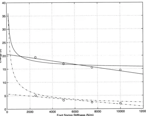
extended. The solid, curved line shows the theoretical energy storage in the spring as calculated for figure 3-6. The solid least-squares line was fit to discrete data points ('o') which represent the energy storage at spring stiffnesses of 2500 N/m, 5000 N/m, 7500 N/m, and 10000 N/m. The dashed, curved line shows the theoretical energy losses in the spring. The dashed least-squares line was fit to discrete data points ('o') which represent the energy losses at spring stiffnesses of 2500 N/m, 5000 N/m, 7500 N/m , and 10000 N/m . . . . 26 3-8 Theoretical and simulated spring efficiencies as calculated from the ratio of energy

lost in damping (i.e. energy absorbed by the knee in simulation) and energy stored in the spring. . . . . 27 3-9 Spring seen by the foot during touchdown with a bent knee. . . . . 28 3-10 Geometry used to calculate virtual spring stiffness. . . . . 29 3-11 Virtual spring stiffness as produced by a constant knee torque. The virtual spring

behaves like a softening spring as the virtual spring compression increases. . . . . 29 3-12 Schematic model of virtual spring in series with foot spring. . . . . 30 3-13 Relationship among force-velocity-compression for the virtual spring. Virtual spring

force is shown in the vertical axis while spring compression and velocity are shown on the two horizontal axis. View I shows the relationship between Virtual Spring Force and Velocity and can be seen in figure 3-15. View II shows the relationship between Virtual Spring Force and Compression and can be seen in figure 3-14. . . . . 31

3-14 Two-dimensional projection of Force versus Compression of virtual spring as seen from View II in figure 3-13. Virtual spring stiffness is shown about the same operating point for motor speeds of 6000, 7000, and 8000 RPM. . . . . 32 3-15 Two-dimensional projection of Force vs. Compression of virtual spring as seen from

View I in figure 3-13. A dashed rectangle shows the normal operating region. . . . . 32 3-16 Energy storage in the foot spring and virtual spring while hopping at 0.25 meters

w ith a bent knee. . . . . 33 3-17 Force seen by the spring during touchdown with a bent knee. . . . . 34 3-18 Energy storage for the fully extended knee and bent knee. For the bent knee case,

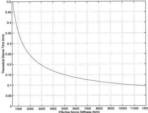
energy storage is the sum of foot spring storage and virtual spring storage . . . . 36 3-19 Theoretical stance time for one legged robot with a springy foot of stiffness from 500

N/m to 12000 N/m calculated using equation 3.33. . . . . 37 3-20 Theoretical and simulated stance time for one legged robot with a springy foot. The

top most figures shows the simulated data 'x' recorded for a fall from 0.25 meters on a fully extend knee. The theoretical data 'o' was calculated using equation 3.33 with

Keff = Kf ,t. The middle figure shows the simulated data recorded for a vertical fall

from 0.25 meters onto a slightly bent knee. The theoretical data 'o' was calculated using equation 3.33 with Kvirt = 6000N/m. The bottom figure shows the simulated data recorded for a running simulation. The theoretical data 'o' was calculated using

equation 3.33 with Kvirt = 6000N/m. .. ... 38

3-21 Theoretical maximum running speed for one legged at varying effective spring stiff-nesses calculated using equation 3.37. . . . . 40 4-1 Standing upright with and without a knee cap. Left shows an unstable buckling

configuration. Center, shows a stable but inefficient configuration. Right shows a stable and efficient configuration . . . . 43 4-2 Swing leg behavior shown with an articulated knee. An initial torque impulse at the

hip swings the thigh forward. The knee joint naturally breaks and the shin swings toward the body to conserve angular momentum. Just before touchdown, a torque impulse is given at the hip joint to bring the thigh to a sudden stop. The shin continues to swing forward eventually being stopped by the knee limit stop. . . . . . 44 4-3 Pendulum driven by a rotary motor. This model is used to represent a typical robot

joint and link. . . . . 44 4-4 Pendulum driven by a rotary motor through a gear reduction. The gear reduction

is necessary on most robot joints to increase the torque and reduce the speed of the

motor... ... 45

4-5 Position control of motor inertia in an attempt to compensate for the effects of re-flected inertia. The angular position of the motor is sensed and compared to the angular position of the pendulum. Any discrepancy between the two measurements will result in a torque on the motor which accelerates the motor inertia toward the position of the pendulum . . . . 46 4-6 A torsional spring has been placed in series between the load (i.e. the pendulum) and

gear reduction. This is known as Series Elasticity and decouples pendulum from motor inertia, allowing for compensation of reflected inertia. Additionally, Series Elasticity can provide accurate torque control of joints and high shock tolerance. . . . . 47 5-1 Joint schematic of a planar quadruped with two degrees of freedom in each leg, a

passive spring at the foot, and a boom to allow body pitch but prevent tipping from side to side (frontal plane). . . . . 50 5-2 Photograph of the experimental robot. Rear leg on the left and front leg on the right. 50

LIST OF FIGURES

5-3 Photograph of planar robot with arrows showing degrees of freedom achievable when

attached to a boom. ... ... ... 51

5-4 Photograph of planarizing boom attached to the two legged experimental robot. . . 51 5-5 Photograph showing the range of motion for the rear knee joint. . . . . 52 5-6 Photograph of showing the range of motion for the rear hip joint. . . . . 53 5-7 Photograph rear leg showing the knee motor location with respect to the hip joint. . 54 5-8 Photograph of the Raibert quadruped showing prismatic knee joints. . . . . 54 5-9 Photograph of the Cheetah Foot used for smooth energy storage and transfer during

running. A string potentiometer is attached to measure compression of the spring. . 55 5-10 Computer rendering of series elastic actuator to be used in the robot. . . . . 57 5-11 Schematic representation of the electronics system of the experimental robot. . . . . 58 5-12 Photograph of electrical components of the robot. Starting in the top left and moving

clockwise: Integrated A/D, D/A, and DSP, motor amplifier, force control board/signal conditioner, analog break out board, power board. . . . . 59 6-1 Representation of equivalent force systems. A single force (shown in the left figure)

can be described by an equivalent force and moment at any location on the beam (shown in the right the figure). . . . . 61 6-2 Representation of equivalent force systems. A vector forces at the center of mass can

be described by torques at the joints. The Jacobian is need to transform forces at the center of m ass to joint torques. . . . . 61 6-3 Schematic of the kinematic configuration of the experimental robot. 0, Ok, and Oh

represent the ankle, knee and hip angles respectively. 0w, 0e, and

0,

wrist, elbow, and shoulder angles respectively.

#arm

upper arm and leg length. L3 is the length from the center of mass to both the hip and shoulder. . . . . 62 6-4 Depiction of an alternate location for virtual forces . . . . 67 6-5 Schematic of the kinematic configuration of the experimental robot. 64 and Oh

repre-sent the knee and hip angles respectively. 0e and

0,

and the foot to the hip, respectively. aarm and

ale,

upper arm and leg length, and L3 is the distance from the hip and shoulder to the center of mass. .. . .. ... .... . ... .... . . . .. . .. . .. .. 68 6-6 Schematic used to transform leg forces into body forces. . . . . 70 7-1 Experimental robot with virtual springs and dampers controlling

fr, f,,

fo.

virtual springs and dampers hold the robot solidly in a standing posture, but are compliant enough to withstand position and force disturbances. . . . . 73 7-2 Control flow of standing algorithm. Robot State Information enters the High-Level

Controller where the state machine determines the state of the robot. Based on the

state, some control action calculates the desired force. Next, the desired force enters

the Low-Level Controller, where the joint torques are calculated using the Jacobian. Finally, the joint torques are applied to the robot and new robot state information is

gathered. ... ... 75

7-3 Left column shows simulated X step response of 0.05 meters with k. = 1000, b_ = 100. Middle column shows simulated Z step response of 0.05 meters with k, = 1000,

b. = 50. Right column shows simulated pitch step response of 0.1 radians with k1hi = 100, b hi = 10. Joint torques and associated joint power are also shown for

the knee, elbow, hip and shoulder in each column. . . . . 76 8

7-4 Left column shows simulated X frequency response at an amplitude of 0.05 meters and frequency of 0.5 hertz with k. = 100, b, = 10. Middle column shows simulated Z frequency response at an amplitude of 0.05 meters and frequency of 0.5 hertz with kz = 1000, b, = 50 Right column shows simulated pitch frequency response at an amplitude of 0.1 radians and frequency of 0.5 hertz with kphi=100, bphi = 10. Joint torques and associated joint power are also shown for the knee, elbow, hip and shoulder

in each colum n. . . . . 78

7-5 Left column shows experimental X step response of 0.05 meters with k, = 1000, b, = 100. Middle column shows experimental Z step response of 0.05 meters with k, = 1000, bz = 50. Right column shows experimental pitch step response of 0.1 radians with kphi = 100, bphi = 10. Joint torques and associated joint power are also shown for the knee, elbow, hip and shoulder in each column . . . . . 79

7-6 Left column shows experimental X frequency response at an amplitude of 0.05 meters and frequency of 0.5 hertz with k, = 100, b, = 10. Middle column shows experimental Z frequency response at an amplitude of 0.05 meters and frequency of 0.5 hertz with k = 1000, bz = 50. Right column shows experimental pitch frequency response at an amplitude of 0.1 radians and frequency of 0.5 hertz with k, hi=100, bphi = 10. Joint torques and associated joint power are also shown for the knee, elbow, hip and shoulder in each colum n. . . . . 81

7-7 State machine used in pronking algorithm. . . . . 82

7-8 x, z, and 0 position of simulated robot over five pronking cycles. . . . . 88

7-9 Data from single pronking cycle for simulated robot. . . . . 90

7-10 Torque data over five pronking cycles for simulated robot. . . . . 91

7-11 Power data over five pronking cycles for simulated robot. . . . . 92

7-12 x, z, and

#

7-13 Power data over five pronking cycles for experimental robot. . . . . 94

List of Tables

5.1 Weight distribution of planar quadruped. . . . . 53

5.2 Detailed joint inform ation . . . . 56

5.3 Physical Properties of Series Elastic Actuator . . . . 57

7.1 Summary of Torque and Power Requirements for Simulated Step Responses . . . . . 75

7.2 Summary of Torque and Power Requirements for Simulated Frequency Responses . . 77

7.3 Summary of Torque and Power Requirements for Experimental Step Responses . . . 77

7.4 Summary of Torque and Power Requirements for Experimental Frequency Responses 80 7.5 State Machine with Sensor Values Indicated . . . . 83

7.6 State Machine and Associated Control Actions . . . . 87

Introduction

Humans have always admired the strength, agility, endurance, and speed of quadrupedal animals. Anyone who has been to a horse track, seen a cheetah run down a gazelle, or witnessed a deer leap over a fence would not likely argue the superhuman quality of these ambulatory feats. In the last century, scientist have begun trying to understand how animals, and quadrupeds in particular, are capable of such tremendous physical challenges, both from a power and control standpoint. By designing and building a robot which attempts to mimic these animals, we hope to better understand the energetics and control of locomotion.

1.1

Goals of Thesis

This thesis addresses the design and control a two legged planar robot to study the quadrupedal locomotion. By restricting the motion of the robot to a plane, quadrupedal locomotion can be closely approximated without the added complexity of four legs and control of balance in three dimensions. The purpose of this robot is four fold:

1. To investigate the use of springs in the feet for smooth and efficient means of energy transfer. 2. To investigate the use of natural dynamics in the swing leg of the robot to achieve high

efficiency.

3. To develop intuitive control algorithms which can easily be scaled to a three dimensional quadrupedal robot.

4. To determine the torque and power requirements for quadrupedal running.

1.2

Summary of Thesis

"

liter-ature which documents the use of biological mechanisms in actual robots. Design recommen-dations to include natural dynamic mechanisms and springs are made.

" Chapter 3 develops guidelines for selecting foot spring stiffness of running robots based on efficiency and controllability of a one legged hopping robot.

* Chapter

4

" Chapter 6 describes Virtual Model Control, comparing it to a puppeteer and a marionette puppet. A Virtual Model Controller is derived for the experimental robot.

CHAPTER 1. INTRODUCTION 12

* Chapter 7 describes algorithms used to control standing and pronking for simulation and

lab-oratory experiments. Standing and pronking experiments are conducted on the experimental robot and power requirements to achieve running are set forth.

Design Inspiration

The design and construction of a robot to study quadrupedal locomotion is a challenging task. The success of such a project requires an understanding of engineering principles and robotics. An understanding of biology is also important because it provides insight into proven mechanical designs and methods of control.

Incorporating mother nature's design elements, such as springs and natural dyanmics, into legged robots is not a new idea. In fact, there are many examples of legged robots using biological mech-anisms to efficienctly walk, run, and even do gymnastics. In this chapter, we investigate the basic biological principals of efficient locomotion and review a few walking and running robots that utilize natural mechanisms to achieve efficient and natural movements. This information is used to generate basic design requirements for the experimental robot to be built.

2.1

Energetics of Walking

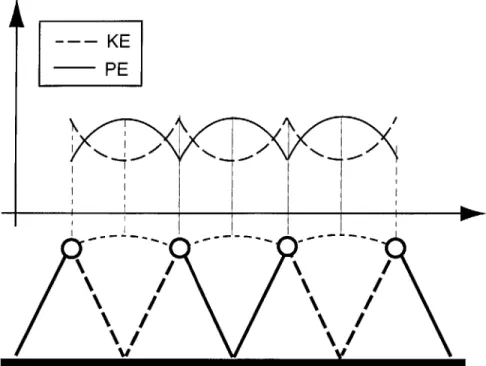
A natural starting point for studying locomotion is the bipedal gait. Specifically, we begin by studying the energetics of a simplified human gait known as the compass gait. The compass gait model consists of two rigid, massless legs attached at the hip with a revolute joint. A point mass is modeled at the hip joint. With only one degree of freedom located at the hip, the body is forced to follow an arc defined by the length of the leg. The compass gait can be seen in figure 2-1.

Since only one foot is in contact with the ground during stance and the body is considered to be a point mass. This gait can be modeled as a simple inverted pendulum. Calculating the external work on the model, namely the potential and kinetic energy of the system, we find

PE = MgLcosO (2.1)

KE = MgL(1 - cosO) (2.2)

Graphing the equations 2.1 and 2.2 in figure 2-1, the cyclical nature of potential energy and kinetic energy can be seen. Note that the kinetic energy is maximum when the potential energy is minimum and vice versa. Similar cyclical transition of potential and kinetic energy was recorded in human subjects by McMahon (1984) using force plate data to calculate the changes in mechanical energy of the body's center of mass.

Intuitively, this exchange of kinetic and potential energy has been likened to an egg rolling end over end [Margaria (1976)]. The egg will speed up and slow down as it gains and losses potential energy. Energetically, this means that no external work is performed if no energy is lost to friction, thus a perfectly efficient gait can be achieved. Of course friction is present in our joints, muscles, and ground contact, so there will be some losses.

CHAPTER 2. DESIGN INSPIRATION

KE

PE

\/

\/

Figure 2-1: Several strides of the compass gait shown with qualitative potential and kinetic energy curves.

Although this model lacks many of the most basic human movements, such as knee and ankle flexion and extension and pelvic tilt and rotation, it is analytically valuable because it demonstrates the cyclical nature of potential and kinetic energy during walking. It is this key feature that makes human walking efficient.

2.2

Energetics of Running

It is known from oxygen consumption measurements on animals that running can be as efficient as walking [McMahon (1984)]. From the study of walking in section 2.1, it can be inferred that efficient running requires a similar cyclical transfer of energy. However, running is dynamically dissimilar to walking for both humans and quadrupeds. Running is defined by a phase when all feet leave the ground. With a little thought, one can see that potential energy and kinetic energy are no longer 180 degrees out of phase as they were in walking. In fact, during running potential and kinetic energy reach a maximum at the peak of the ballistic phase and a minimum sometime during touchdown.

Since the animal cannot transfer kinetic and potential energy back and fourth as was the case in human walking, some other mechanism must be used to store energy and achieve efficient running gaits. In fact, animals use their muscles and tendons to store elastic energy at touchdown and release it before lift-off. In this way, animals reduce the external work required during running. With the power limitations of todays motors, it is imperative to design similar elasticity into our robot if we want it to be able to run at all.

It is believed that animals not only use elastic storage at touchdown, but also during other phases of running. For example, Alexander (1990) believes that it is feasible that animals use elastic storage elements to quickly and efficiently reverse the angular velocity of the leg while transitioning from stride to swing and vice versa (see figure 2-2). Alexander (1990) also believes that animals may use soft foot pads to reduce the high impact forces experienced while running. Furthermore, foot pads 14

Figure 2-2: Springs used to efficiently reverse the direction of robotic leg.

may also be used to reduce high frequency vibrations of the foot on the ground, known as chatter. Clearly, springs play an important role in running of animals.

Springs have been used as energy storage devices in several robots to date. Most notable were the use of pnuematic springs in one, two and four legged running and hopping robots by Raibert [Raibert. (1986)]. Carrying this idea forward, Buehler (1996) developed a monopod with a springy foot, similar to the one used in Raibert's one legged hopper, and hip return springs, as in figure 2-2. The monopod had an average power consumption of only 125W, making it much more efficient than its predecessors.

2.3

Natural Dynamics

Another important mechanism that is used by animals to achieve efficient running and walking gaits is natural dynamics. Natural dynamics describe the use of natural, unactuated motions to achieve controlled movements. As a simple example, a pendulum clock uses its natural dynamics, dictated by the mass and length of the pendulum and the local gravity constant, to keep track of time. The pendulum is given tiny pulses of energy at the both extremities of the swing when the velocity is zero. Between these pulses, the natural natural dynamics of the system take over and move it to the next state. In this way, a pendulum clock is a very efficient mechanism.

This example is not dissimilar from the way we use natural dynamics to walk. At the beginning of swing phase, we give our hip an impulse of energy and then let the natural pendulum motion carry it forward to extension. Just before extension, we give the hip another tiny impulse of energy in the opposite direction to bring it to a sudden halt before touchdown. Electromyographic data records by McMahon (1984) show little electrical activity in the leg muscles of humans during the swing phase at normal walking speeds. This, of course, suggests that the leg is swinging freely during this period. As a sanity check, electromyographic records show significant electrical activity in leg muscles during stance.

Natural dyanmics have also found there way into many robots. Much research has been done on completely passive walking machines [Garcia et al. (1998), Adolfsson et al. (1998), Fowble & Kuo (1996), McGeer (1990)]. Passive walking robots use Earth's gravity as a power supply and rely on special geometry to achieve gaits similar to the compass gait described in figure 2-1. By exploiting natural dynamic elements, a robot can achieve a high overall efficiency. In the limit, a robot can rely entirely on natural dynamic motions and thus require no external power source. Natural legged robots such as these have been constructed and successfully demonstrated.

Natural dynamics were successfully implemented in actuated robots as well. Pratt & Pratt (1999) developed algorithms that use the natural dynamics of the swing leg to efficiently control a planar bipedal robot. More recently, Pratt has developed three-dimensional simulations of a bipedal walking robot using natural elements such as a knee stop, compliant ankle, and passive swing leg to

CHAPTER 2. DESIGN INSPIRATION

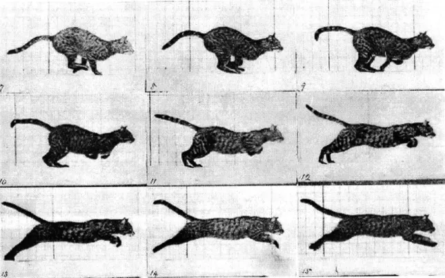
Figure 2-3: Galloping cat as photographed by Eadweard Muybridge. Frame 7-15 of plate 128. Reprinted with permission from Dover Publications.

achieve natural looking and efficient walking.

Gymnastic maneuvers have also been accomplished in several robots using natural dynamic principals. Hodgins (1987) used natural dynamics to get a two legged planar robot to do a forward flip while running. Playter (1995) used the natural dynamics of springy arms to successfully control layout somersaults of a wooden doll.

2.4

Other Important Biological Elements

Yet another biological mechanism that is important to the animal during running is back flexion. Back flexion is shown dramatically in photographs by Muybridge [Muybridge (1957)] in figure 2-3. By flexing and extending its back, the cat in the picture is gaining two advantages. First, it is significantly lengthening its stride length and thus increasing its speed. Second, it has been pointed out that back flexion allows the animal to place its foot closer to the center of gravity projection of the body [Raibert. (1986)). This feature gives the animal a higher degree of stability when only one foot is contacting the ground. It has also been suggested that the back may be acting as an elastic storage device as we discussed in 2.2.

Little research has been done in this area, with the exception of Leeser (1996) who used an articulated spine to successfully control a planar quadrupedal robot.

2.5

Design Recommendations

From this literature survey, one can clearly see that a cyclical energy transfer mechanism is imper-ative for efficient running. As such, a springy element, which will provide smooth energy transfer

during running will be designed into the experimental robot. Spring selection will be discussed in chapter 3 Also, it is apparent that natural dynamics play an important role in efficient and natu-ral locomotion, thus natunatu-ral dynamic mechanisms will be considered. Designing natunatu-ral dynamic elements will be detailed in 4. Finally, the literature review also suggest that a springy back can po-tentially provide more energy storage and natural movements. However, because of the complexity such an element would add to the design, it has been delayed for possible future work.

Chapter 3

Spring Selection

From the study of the energetics of walking and running, as reviewed in Chapter 2, we know that smooth energy transfer is critical for efficient locomotion. In walking, the energy is naturally cycled between kinetic and potential energy due to the geometry of walking gaits. During running, poten-tial and kinetic energy are nearly in phase, requiring a much different energy transfer mechanism. Springs, in the form of tendons, and to some extent muscles, provide the compliance necessary for smooth storage and transfer of kinetic and potential energy during running.

Designing compliance into running robots is not an easy task. Tendons are highly efficient, light weight springs with non-linear properties. Furthermore, animals have the ability to change their compliance depending on environmental conditions. Clearly, we will be unable to replicate such complex behavior with the springs available to us. However, with a little thought, we can make wise decisions when selecting a spring that will result in a robot that is both energy efficient and controllable.

In this chapter we investigate the choice of linear spring stiffness for both efficiency and con-trollability of a one legged hopping and running robot. A one legged robot is simulated because its energetics and control can easily be applied to bipedal and quadrupedal robots [Raibert. (1986)]. This task can be divided into two phases: modeling and simulation.

In the modeling phase, we develop an ideal mass-spring model to understand energy storage in springs and place an upper bound on the maximum energy storage possible. Next, a realistic model is developed which includes spring losses and mass distribution. This mass-spring-damper system closely models the one legged robot used in the simulation phase. In this way, the realistic model provides base-line data to insure the validity of data collected from our simulated robot.

After a thorough understanding of expected spring behavior is developed, simulation experiments are conducted on a one legged hopping robot with a springy foot and articulated knee. A schematic of the one legged robot can be seen in figure 3-1. First, a simulation experiment is conducted to check for agreement between the mathematical model and the simulated robot. After verification, the efficiency of the robot is tested during a hopping experiment. Next, controllability is investi-gated during hopping and running experiments. Based on these results, recommendations are made regarding the selection and efficient use of springs in running and hopping robots.

3.1

Modeling

3.1.1

An Ideal Model

As a first pass at modeling the one legged robot, the spring in the foot is assumed to be massless and lossless. The ideal model can be seen in figure 3-2. From this model, we can calculate the maximum energy savings that can be realized with springs in running robots.

The total energy at any moment in time can be written as

Fully Extended Knee Bent Knee

Figure 3-1: One legged hopping robot used in simulation. The robot possess a revolute hip joint with an articulated knee and springy foot.

eM htd

K

M

_e

_

hl,

K

Figure 3-2: Mass-spring system representing a simple one-legged hopping robot of figure 3-1 in the fully extended knee configuration. For the ideal model, the mass is assumed to be a point mass, while the spring is assumed to be massless and lossless. This model will provide the maximum energy storage possible.

CHAPTER 3. SPRING SELECTION

Etotai = Epotentiai + Ekinetic + Espring (3.1)

Just before the foot of the simplified model touches the ground the total energy is 1

Etd = Mghtd +

2MVtd

Just before the robot begins lift-off, the foot spring is fully compressed and vertical velocity is zero, resulting in a total energy of

1

E10 = Mghlo + 0 + 2Kx1o (3.3) Since energy is conserved, we can equate equations 3.2 and 3.3 and solve for the energy storage in the spring.

1 2 _{1 2}

2Kx10 = Mg(htd - hio) + 2Mvtda (3.4)

From equation 3.4, it can be seen that the maximum energy storage in the spring is equal to the kinetic energy just before touchdown and the change in potential energy from touchdown to lift-off. If no foot spring is present, all of this energy will be dissipated by the ground. Immediately, we can see the significant energy savings springs provide.

Equation 3.4 provides an qualitative value of energy storage, but it is useful to have a quantitative measure of the maximum spring storage. To do this, we need to solve the second-order differential equation which represents the spring-mass model in figure 3-2.

M = -Kx + Mg

The solution is of the form

x =Cisin(wt)

+

= CiWncos(wnt) - C2wnsin(Wnt)

(3.7)

(3.8) Using the initial conditions

x(0) 0

(O) =u = V2gh

(3.9) (3.10) and substituting x(0) and ±(0) into equation 3.6 and 3.8 respectively, and solving for C₁ and C2

yields

0.2 1 0.18 0.16 0.14 0.12 16 E a 0 *N 0.1 0.1 E 80.08 x 0.06 0.04 0.02 K=5000 K i7500 -.. . .-.. ...-.. - ....-. -. -.-.-. ... ... .- .- -. -

~ ~ ~ ~ ~~~~

~ ~

~

~

~

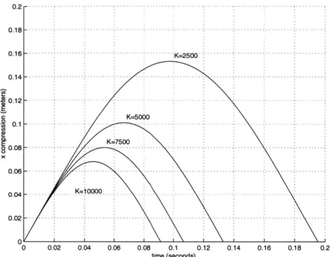
Figure 3-3: Maximum spring compression calculated using equation 3.11 with initial conditions

x(0) = 0.0 and ±(0) = N/2gT where h=0.25 meters, M=7.33 kg, and K is a varying stiffness labeled on each plot above.

v/_g Mg

x = sin(wt) + 7g(1 - cos(Wnt))

W, K (3.11)

From equation 3.11, we can calculate the compression of the spring for a range of spring constants. This data can be seen in figure 3-3. It is not surprising that softer spring constants result in larger spring compression.

The energy storage of a spring can be written as

Espring = 1 ₂

Kx

Again, using equation 3.11 to calculate the maximum spring compression and substituting into equation 3.12 we find the maximum energy storage in the spring. This value has been plotted for spring stiffness up to 12000 N/m in figure 3-4. It should be noted that since there are no losses in the system, figure 3-4. represents the maximum energy storage possible in the spring. To check the validity of this result, equation 3.4 has also been plotted in figure 3-4. It cannot be seen because it is coincident with the maximum energy stored in the spring.

At first glance, intuition tells us that since there are no losses in our theoretical model, all springs stiffnesses should store the same amount of energy. However, closer investigation of equation 3.4 reveals that the energy stored in the spring is a function of spring stiffness. Consider two cases:

1. For a stiff spring, the maximum compression will be small, thus the difference between htd and h1, will be small, resulting in a small APE.

CHAPTER 3. SPRING SELECTION

2000 4000 6000 Foot Spring Stiffness (N/rn)

8000 10000 12000

Figure 3-4: Maximum energy storage in foot spring for a mass of 7.33 kg dropped from a height of 0.25 meters. Calculated by combining equations 3.11 and 3.12. A massless spring with no damping is assumed.

2. For soft spring, the maximum compression will be large, thus the the difference between htd

and hl0 will be large, resulting in a large APE and more energy storage.

Since the kinetic energy of the system just before touchdown is constant, and if we assume equal efficiency for all spring stiffnesses, then it follows that as stiffness increases, spring energy storage will decrease. This conclusion agrees with the data seen in figure 3-4. Prom here forward, this effect will be known as the APE Effect.

The question remains: how does spring storage relate to efficiency of the system? Initially, one might presume that more energy storage in the foot spring results in a more efficient spring-mass system. In fact, this is not the case. Even though a soft spring stores more energy than a stiff spring, all masses will rebound to the same height because the greater energy storage in the soft spring comes at the expense of potential energy. Said another way, the soft spring stores more en-ergy during touchdown, but must provide that extra enen-ergy during lift-off to rebound to the original height.

To summarize the important features of the ideal model:

* Springs are capable of storing all of the kinetic energy and change of potential energy of a spring-mass system.

* Kinetic energy is dependent only on initial height, not spring stiffness.

* Potential energy storage is larger for soft springs than for stiff springs. This has been dubbed the APE Effect.

e As a result of the APE Effect, the total energy storage will decrease with increasing spring stiffness as seen in figure 3-4.

40 35 30 25-220 C 15 10 [- - - - ----.-. -5 0 22 . . . ... .. . . ... . . .. . . . . . . .... . . . . . . . .. . . . .. . . . . . . ... . . . . .. ... ... ... ...

M

Musprung

Figure 3-5: Model of one legged hopping robot including the effects of damping, distributed mass of the links, and the unsprung mass of the spring.

e Even though energy storage decreases as stiffness increases, the energy efficiency of the system, in this case a spring and mass, is independent of spring constant.

3.1.2

A Realistic Model

The lossless and massless model of section 3.1.1 is an excellent starting point to begin studying the use of compliance in running robots. It provides an upper-bound on the amount of energy savings that can be realized in a robot with compliance and provides insight into basic spring behavior. Unfortunately, because the simplified mass-spring model ignores the distributed mass and losses of our simulated robot, it cannot provide an accurate prediction of spring and robot behavior. The simulated robot, as can be seen in figure 3-1, is significantly different than the simple spring-mass model of figure 3-2 in three ways.

1. The simulated robot has damping due to friction at the knee joint and losses in the foot spring. Energy dissipation due to damping will result in less than maximum energy storage.

2. The mass of the simulated robot is distributed in the links and the body. Distribution of the mass in the leg and spring will lower the center of gravity of the robot, decreasing its potential energy as compared to the point mass in the first mass-spring model of figure 3-2.

3. Since our spring is no longer massless, we must include the losses due to its unsprung mass. Unsprung mass is defined as the mass which comes instantly to zero velocity when striking the ground. The robot will lose all of the kinetic energy associated with the unsprung mass when it strikes the ground.

These differences can be added to our spring-mass model to provide a more accurate base-line to compare simulation data. Figure 3-5 shows damping, distributed mass, and unsprung mass added to the simple model.

To quantify the effects of the damper, we need to solve a second-order differential equation very similar to equation 3.5

M. = -B - Kx + Mg (3.13)

The solution is of the form

CHAPTER 3. SPRING SELECTION 24

where

Wd = ( 2M (3.15)

-B

a = _{a 2M} (3.16)

Taking the derivative of equation 3.14 yields

i

Using the initial conditions

x(0) 0 (3.18)

±(0) u = = 2gh (3.19)

and substituting x(0) and -(0) into equation 3.14 and 3.17 respectively, and solving for C1 and

C₂ yields

V2 - _ -B Mg -B

x = 2' eTMtsin(wdt) + (1 - e '7'cos(wdt)) (3.20)

Wd K

As a check, setting B=0 in equation 3.20 yields equation 3.11.

From equation 3.20 and its derivative, we can calculate the spring energy storage with a damper in the system according to

1 2

Espring = Kx2 - B2 (3.21)

2

Assuming constant damping of 25 kg/s, the energy storage, adjusted for damping, can be seen as the dashed line in figure 3-6 labeled Estored (Adjusted for Damping).

Distributing the mass to the leg and spring of the robot also requires adjustments to our original model. The center of gravity of the robot with distributed mass is 0.055 meters below the original point mass. This reduces the potential energy according to PE = Mgh. This accounts for 3.95 Joules. This is a constant effect, so we can just subtract 3.95 Joules from the energy stored at all spring stiffness.

The unsprung mass has been modeled to be 0.1 kg. Every time the spring strikes the ground the unsprung mass dissipates its kinetic energy to the ground according to KE = !Mv2 . This accounts

for a loss of about 0.25 Joules on each cycle. Again, this can simply be subtracted from the energy stored at all spring stiffness.

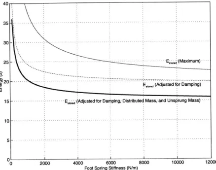
Thus, the total adjustment due to the distributed mass and unsprung mass is a loss 4.20 Joules. This has been subtracted from energy storage curve adjusted for damping. The final result can be seen in figure 3-6 as the bold line labeled Estored (Adjusted for Damping, Distributed Mass, and

Unsprung Mass). This curve will provide the baseline to verify our simulation results. To summarize the important features of the realistic model:

* The energy storage curve for the realistic model is very similar in shape to the energy storage curve for the ideal model, but is shifted down approximately 5.0 Joules to account for damping and an additional 4.2 Joules to account for distributed mass in the links and the unsprung mass of the spring.

3 3' 2 2 aU 1 0 2000 4000 6000

Foot Spring Stiffness (N/m) 8000 . .. ... .... -.-.-. .-- (M axim um ) -0... 71 -_-_---05 . . . ... . . . ....

E.r (Adjusted for Damping)

5 -.. -E - - E Adjustedfor Daping Distributed Massand Unsrung Mass).

slm

12000

Figure 3-6: Energy storage shown for no losses, adjusted for damping (dashed line), and adjusted for damping, distributed mass, and unsprung mass (bold line).

3.2

Simulation

3.2.1

Verification of Simulation

To verify the agreement of the realistic model and the simulated robot, a simple simulation ex-periment is conducted. The simulated robot is dropped from a height of 0.25 meters with a fully extended knee onto foot spring stiffnesses of 2500 N/m, 5000 N/m, 7500 N/m, and 10000 N/m and constant damping term of b=25 kg/s. With these initial conditions, the simulation data should match the realistic model well. The results of the simulation experiment can be seen in figure 3-7.

Reasonable agreement can be seen between the theoretical energy storage and the least squares fit to the simulated energy storage. Discrepancies between the two models can be explained by errors caused by estimations in the distributed mass of the robot. Excellent agreement can be seen between the theoretical energy dissipated and the least squares fit to the simulated energy dissipated. Efficiency, as defined in equation 3.22, is also a good measure to verify the agreement between theoretical and simulated results.

Ef

ficiency

)

Efficiency has been graphed in figure 3-8. Nearly perfect agreement can be seen between theo-retical and simulated efficiencies.

With this experiment, we conclude that our model is an accurate representation of the simulated robot. From here forward, we will use the least-squares fit lines in figure 3-7 as the base-line to compare future simulation results.

An

CHAPTER 3. SPRING SELECTION 26 40 35- -- - - - -- -~ 30 - - -2120 - -- -. . . 10 1 0 . . . . .. . . . . . .. . . . . . . . . . 0 2000 4000 6000 8000 10000 12000

Foot Spring Stiffness (N/m)

Figure 3-7: A simulated robot was dropped from a height of 0.25 meters with the knee fully extended. The solid, curved line shows the theoretical energy storage in the spring as calculated for figure 3-6. The solid least-squares line was fit to discrete data points ('o') which represent the energy storage at spring stiffnesses of 2500 N/m, 5000 N/m, 7500 N/m, and 10000 N/m. The dashed, curved line shows the theoretical energy losses in the spring. The dashed least-squares line was fit to discrete data points ('o') which represent the energy losses at spring stiffnesses of 2500 N/m, 5000 N/m, 7500 N/m, and 10000 N/m.

ul I 1~~~~~

. . . .. . . .

.

0

x

6000 Foot Spring Stiffness (N/m)

.. . . .

Theoretical Efficiency

-Experimental Efficiency

8000 10000

Figure 3-8: Theoretical and simulated spring efficiencies as calculated from the ratio of energy lost in damping (i.e. energy absorbed by the knee in simulation) and energy stored in the spring.

3.2.2

Efficiency Analysis and Simulation

With a clear understanding of expected spring behavior and a verified model of a hopping robot, we can now consider the issue at hand: selection of foot spring stiffness. First, we will consider selection of foot spring stiffness based on efficiency of a hopping robot.

Due to inherent losses in the system, the one legged hopping robot must inject energy into the system to maintain hopping height. This is achieved by thrusting with knee or hip torque during stance. Assuming that the hip torque is used only for adjustment of body pitch, then if the knee is fully extended at touch down, the robot has no way of pushing on the ground to maintain hopping height. Thus, the one legged hopping robot, which uses hip torque only for adjustments in body pitch, must land with a bent knee if hopping height is to be maintained. Unfortunately, landing with a bent knee affects the energy storage in the spring in two ways:

" In order to store energy in the foot spring, the bent knee must present a very high impedance to the foot spring. The maximum impedance is limited by speed-torque curves of the motor driving the knee joint. The impedance produced by the knee joint and seen at the foot spring is described by a virtual spring of varying stiffness. This is called the Virtual Spring Effect and is described in detail in section 3.2.3.

" Because of geometry, the bent knee reduces the maximum energy storage possible in the foot spring. This is called the Alpha Effect and is described in detail in section 3.2.4.

3.2.3

The Virtual Spring Effect

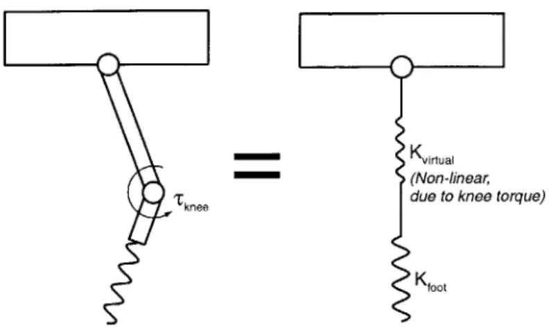
First, we consider the affects of the virtual spring on efficiency. A proportional controller at the knee (rknee KpOknee) looks like a virtual spring between the foot and the hip. This situation can

10 90 k . . . .. . . . .. . 80 - .-.-.- . 70 -.- . 601-C 50 F 40 -. 30 - .- .- . 20H -- - -- - - - -10

-F

CHAPTER 3. SPRING SELECTION 28

T knee

Figure 3-9: Spring seen by the foot during touchdown with a bent knee.

be seen in figure 3-9 The virtual spring stiffness can be calculated using the geometry in figure 3-10. Assuming a constant torque at the knee we find that the virtual spring force is

Lsin ( "k)

The compression of the virtual spring can be written as

xvirtual - 2L 1 - cos Oknee

(3.23)

(3.24) Using equations 3.23 and 3.24, a curve showing the characteristics of the virtual spring behavior has been graphed and can be seen in figure 3-11. We can see that the virtual force approaches infinity at zero spring compression (Okne =0.0) and sharply decreases as virtual spring compression increases.

Thus, for a constant torque the virtual spring behaves like a softening spring as compression increases

(Oknee increases).

Two springs of different stiffness in series, as in figure 3-12 will not equally distribute energy storage. Using force equilibrium on the springs we find

F1 = Kjxi = K2x2 (3.25)

Solving for xi and x2 we find

F₁ K₁ F₁ x₂ = (3.26) (3.27) The energy storage in each spring is

Kyirtual

(Non-linear, due to knee torque)

Figure 3-10: Xiu=2L-2Lcos -) I L -j (Oknee

CJIj

Geometry used to calculate virtual spring

Oknee (Degrees)

0 26.5 37.5 46.1 53.4 59.8 65.6 71.0 76.2 81.0 85.6

U

0 0.02 0.04 0.06 0.08 0.1 0.12 0.14 0.16 0.18 0.2 Virtual Spring Compression (m)

Figure 3-11: Virtual spring stiffness as produced by a constant knee torque. The virtual spring behaves like a softening spring as the virtual spring compression increases.

stiffness. -. -. .. .. . . - .. . -. -. -. . .. . . . .-. .-.-. .-. .-.-....-. .-. .-. .--~... -. -.--. _n....s. 5000 4500 4000 3500 3000 2500 32000 1500 1000 500

CHAPTER 3. SPRING SELECTION 30

F1

K

K-1 2

Figure 3-12: Schematic model of virtual spring in series with foot spring.

1 2 I K, 2 2 K1 F2_F1 (3.28) 2K 1 1 2 E2 = -K2X2 2 1 _(3.29) 2K2

From equations 3.28 and 3.29, we can see that the softer of the two springs will store more energy than the stiffer spring. In this way, the foot spring competes with the virtual spring to "store" energy. We say "store" energy when referring to the virtual spring because the virtual spring cannot actually store energy, rather, it can only dissipate energy. Clearly, we want the foot spring to win this competition, but who does win?

To answer this question, we must place a value on the maximum virtual spring stiffness. Virtual spring stiffness is limited by the torque-speed characteristics of the motor which generates the virtual spring. That is to say, the virtual spring may not exceed the power of the motor. The torque-speed curves of the motor have been mapped to force-velocity-compression curve of the virtual spring. A third dimension, spring compression, is needed to map the motor's torque-speed curve to the virtual spring power curve because both the velocity and force of the virtual spring depend on virtual spring compression. Figure 3-13 shows the relationship among force-velocity-compression for the virtual spring. Immediately, we see that virtual spring force decreases with increasing compression and increasing velocity. Intuitively, this makes sense. As compression increases the knee losses mechanical advantage. As velocity increases, force must decrease due to power limitations on the motor.

The virtual spring stiffness at any point can be measured from the slope of the force versus compression curve as seen by viewing from View II in figure 3-13. The two-dimensional projection of View II can be seen in figure 3-14. To deduce the virtual spring stiffness, one needs to specify both a virtual spring compression and an appropriate motor speed curve.

Virtual spring compression is approximately 0.05 meters at touchdown. Recall, it is necessary to land with a bent knee ( virtual spring compression > 0.0 ) in order to be able to provide energy during lift off. This operating point can be seen as a dashed vertical line in figure 3-14

View I

2000,

- - - - -High Speed /Low Torque

d1500c- inHigh Low Speed Torque

1000, -500, --0 -2.5 005 -21 9, 617 0 15 _{0.2 0} 0.5 ₀

Figure 3-13: Relationship among force-velocity-compression for the virtual spring. Virtual spring force is shown in the vertical axis while spring compression and velocity are shown on the two horizontal axis. View I shows the relationship between Virtual Spring Force and Velocity and can be seen in figure 3-15. View II shows the relationship between Virtual Spring Force and Compression and can be seen in figure 3-14.

CHAPTER 3. SPRING SELECTION 0. C 7t 2000 1800 160( 140 120 100 80 60 40 20 32 0 0.02 0.04 0.06 0.08 0.1 0.12 0.14 0.16 0.18 0.2

Virtual Spring Compression (m)

Figure 3-14: Two-dimensional projection of Force versus Compression of virtual spring as seen from View II in figure 3-13. Virtual spring stiffness is shown about the same operating point for motor speeds of 6000, 7000, and 8000 RPM. 9 2 0, CD .9, CL 1.5 F 0.5 00 0.02 0.04 0.06 0.08 0.1 0.12 0.14 0.16 0.18 0.2

Virtual Spring Compression (m)

Figure 3-15: Two-dimensional projection of Force vs. Compression of virtual spring as seen from View I in figure 3-13. A dashed rectangle shows the normal operating region.

-- High Speed / Low Torque

- --- _{Low Speed / High Torque}

Operating Point

2

-K.=4.. _{.... ...} M

0

--- High Speed/ Low Torque

- Low Speed /High Torque

-

-Normal Operation

i000

1